www.biogeosciences.net/10/4591/2013/ doi:10.5194/bg-10-4591-2013
© Author(s) 2013. CC Attribution 3.0 License.
Biogeosciences
Geoscientiic
Geoscientiic
Geoscientiic
Geoscientiic
The influence of temperature and seawater carbonate saturation
state on
13
C–
18
O bond ordering in bivalve mollusks
R. A. Eagle1,2, J. M. Eiler2, A. K. Tripati1,3, J. B. Ries4, P. S. Freitas5, C. Hiebenthal6, A. D. Wanamaker Jr.7, M. Taviani8,9, M. Elliot10, S. Marenssi11, K. Nakamura12, P. Ramirez12, and K. Roy13
1Department of Earth and Space Sciences, University of California, Los Angeles, CA 90095, USA
2Division of Geological and Planetary Sciences, California Institute of Technology, Pasadena, CA 91125, USA
3Department of Atmospheric and Oceanic Sciences, Institute of the Environment and Sustainability, University of California, Los Angeles, CA 90095, USA
4Department of Marine Sciences, University of North Carolina-Chapel Hill, Chapel Hill, NC 27599, USA
5Divis˜ao de Geologia e Georecursos Marinhos, Instituto Portuguˆes do Mar e da Atmosfera (IPMA), Av. de Bras´ılia s/n, 1449-006 Lisbon, Portugal
6Helmholtz Centre for Ocean Research (GEOMAR), D¨usternbrooker Weg 20, 24105 Kiel, Germany 7Department of Geological and Atmospheric Sciences, Iowa State University, Ames, IA 50011, USA 8ISMAR-CNR, Via Gobetti 101, 40129 Bologna, Italy
9Biology Department, Woods Hole Oceanographic Institution, 266 Woods Hole Road, Woods Hole, MA 02543, USA 10Universit´e de Nantes, CNRS UMR6112, Laboratoire de Plan´etologie et G´eodynamique, rue de la Houssini`ere, Nantes, France
11Instituto Ant´artico Argentino, Cerrito 1248, C1010AAZ Buenos Aires, Argentina
12Department of Geological Sciences, California State University, Los Angeles, CA 90032, USA 13Division of Biological Sciences, University of California, San Diego, CA 92093, USA
Correspondence to:R. A. Eagle ([email protected])
Received: 14 December 2012 – Published in Biogeosciences Discuss.: 4 January 2013 Revised: 5 May 2013 – Accepted: 27 May 2013 – Published: 10 July 2013
Abstract. The shells of marine mollusks are widely used archives of past climate and ocean chemistry. Whilst the mea-surement of molluskδ18O to develop records of past climate change is a commonly used approach, it has proven challeng-ing to develop reliable independent paleothermometers that can be used to deconvolve the contributions of temperature and fluid composition on molluscan oxygen isotope compo-sitions. Here we investigate the temperature dependence of 13C–18O bond abundance, denoted by the measured param-eter147, in shell carbonates of bivalve mollusks and assess its potential to be a useful paleothermometer. We report mea-surements on cultured specimens spanning a range in wa-ter temperatures of 5 to 25◦C, and field collected specimens spanning a range of−1 to 29◦C. In addition we investigate the potential influence of carbonate saturation state on bi-valve stable isotope compositions by making measurements on both calcitic and aragonitic specimens that have been
1 Introduction
Molluscan carbonate was amongst the first biologically pre-cipitated materials investigated during the development of the oxygen isotope paleotemperature scale (Epstein et al., 1953). Subsequently fossil mollusks have been widely used as an archive of past environmental change and seawater chemistry (e.g., Keith et al., 1964; Killingley and Berger, 1979; Grossman and Ku, 1986; Taviani and Zahn, 1998; Veizer et al., 1999; Tripati et al., 2001; Tripati and Zachos, 2002; Ivany et al., 2008; Wanamaker et al., 2011). How-ever it has proven challenging to develop robust independent paleothermometers in mollusk carbonate; for example, ap-proaches using trace element partitioning (Mg / Ca, Sr / Ca) into mollusk shell carbonate are often hampered by strong bi-ological controls and high inter- and intra-specimen variabil-ity (e.g., Dodd, 1965; Lorens and Bender, 1980; Klein et al., 1996; Gillikin et al., 2005; Freitas et al., 2006, 2008, 2009; Heinemann et al., 2011; Wanamaker et al., 2008). Therefore it has not yet been possible to reliably partition the contri-butions of temperature and seawaterδ18O to bivalve mollusk carbonateδ18O with a high level of confidence in environ-ments where both parameters could be expected to vary.
“Clumped” isotope paleothermometry is an emerging ap-proach for reconstructing the temperatures of carbonate min-eral precipitation (Eiler, 2011). The technique is founded on the principle that rare isotopes of carbon and oxygen have a thermodynamically driven tendency to bond with each other, or “clump”, and that this effect increases as temperature de-creases (Wang et al., 2004; Schauble et al., 2006). In prac-tice the abundance of13C–18O bonds in carbonate minerals is measured from the abundance of mass-47 CO2 (predom-inantly13C18O16O) liberated on phosphoric acid digestion of carbonate minerals (Ghosh et al., 2006). Measured values are compared to a reference frame where isotope abundances from sample gases are compared to reference gases that have been heated to 1000◦C, producing a nearly random distribu-tion of isotopes among all isotopologues (Eiler and Schauble, 2004; Affek and Eiler, 2006; Huntington et al., 2009; Passey et al., 2010). More recently, standardization to CO2 equili-brated with water at two or more controlled temperatures has been proposed as an “absolute reference frame” in an effort to reduce interlaboratory differences due to mass spectro-metric effects such as bond breaking and reordering during sample gas ionization (Dennis et al., 2011). Here we refer to data presented relative to heated gases only as “relative to the stochastic distribution” although this reference frame has also been described as the “Caltech intralab reference frame” as strictly speaking our heated gases do not reach the full stochastic distribution (Ghosh et al., 2006; Huntington et al., 2009). Data presented relative to the newly proposed reference frame is referred to as being on the “absolute ref-erence frame” (Dennis et al., 2011). In both cases, we report data using the147parameter, which expresses the abundance of 13C–18O bonds found in a sample as an enrichment, in
per mil, above that expected if isotopes were distributed ran-domly (Eiler and Schauble, 2004; Huntington et al., 2009).
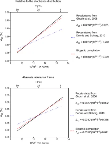
Following the calibration of the clumped isotope ther-mometer in inorganically precipitated calcite (Ghosh et al., 2006) detailed calibration studies of foraminifera, coccol-iths, tooth bioapatite, and corals from our laboratory have shown that these biologically precipitated materials appear to yield a relationship between147and temperature (Fig. 1) that is very similar to inorganic calcite (Tripati et al., 2010; Eagle et al., 2010; Thiagarajan et al., 2011). The close re-lationship between the inorganic calcite calibration and147 data from foraminifera, coccoliths, and corals – even in taxa that show deviations of up to ∼4 ‰ from theδ18O values expected given the temperature andδ18O of the fluid from which they precipitate – suggests either that inorganic calcite and biogenic carbonates are close to equilibrium or that all exhibit non-equilibrium effects of similar magnitude. In con-trast, a study on otoliths and data from a singlePoritescoral specimen exhibit deviations from the inorganic calibration line (Ghosh et al., 2006, 2007). In the case of otoliths this could be explained by uncertainties on the precise formation temperature of the samples, as appears to be also a factor in measurements on thermocline dwelling foraminifera (Tri-pati et al., 2010), or due to small systematic analytical errors that were likely more common early in the history of147 measurements. The difference betweenPoritescoral and the inorganic calibration in Ghosh et al. (2006) is relatively large and could be the result of a growth rate related “vital effect” (Saenger et al., 2012).
It is unclear why some biogenic carbonates exhibit rela-tionships between temperature and147that resemble the in-organic calibration of Ghosh et al. (2006) whereas other bio-genic materials do not. It is possible that this difference in behavior will shed new light on the long-standing problem concerning the origin of stable isotope “vital effects” (Weiner and Dove, 2003); namely, differences in isotopic composi-tion between biogenic materials and composicomposi-tions expected for thermodynamic equilibrium with their environment. Var-ious explanations have been advanced for vital effects on the
9 10 11 12 13 14 0.50
0.55 0.60 0.65 0.70 0.75 0.80
50 25 1
T (°C)
Relative to the stochastic distribution
Recalculated from Ghosh et al., 2006
Δ47 = 0.0598*(106*T-2)-0.025
Recaclulated from Dennis and Schrag, 2010
Δ47 = 0.0316*(106*T-2)+0.267
Biogenic compliation
Δ47 = 0.0550*(106*T-2)+0.027
106/T2 [T inKelvin]
Δ47
(
‰
)
9 10 11 12 13 14 0.55
0.60 0.65 0.70 0.75 0.80 0.85 0.90
50 25 1
T (°C)
Recalculated from Ghosh et al., 2006
Δ47 = 0.0620*(106*T-2)+0.002
Absolute reference frame
Biogenic compilation
Δ47 = 0.0559*(106*T-2)+0.071 Recalculated from Dennis and Schrag, 2010
Δ47 = 0.0340*(106*T-2)+0.316
106/T2 [T in Kelvin]
Δ47
(
‰
)
Fig. 1.Published calibrations of the carbonate clumped isotope
ther-mometer. The top panel shows previously published inorganic cal-ibration lines relative to the stochastic distribution, as described by Huntington et al. (2009) as well as a recalculation of the regression through the data compilation of Tripati et al. (2010) which drew on several original sources (Ghosh et al., 2006, 2007; Came et al., 2007; Eagle et al., 2010; Tripati et al., 2010); and now has the data from Thiagarajan et al., included (Thiagarajan et al., 2011). Data from Zaarur et al., was not included due to uncertainties over ex-actly what environmental conditions the materials analyzed should reflect (Zaarur et al., 2011), and thePoritescoral analyzed by Ghosh et al., was also excluded due to apparent kinetic isotope effects on
147values (Ghosh et al., 2006). Also shown is a regression through
the same compilation of published materials now converted into the absolute reference frame (Table S1) via the secondary transfer function method (Dennis et al., 2011). Note that the 106/T2scale withT in degrees Kelvin is the primary temperature scale used for data plots, with a secondary x-axis in degrees Celsius presented as a guide only. All regression lines were recalculated from original data (see methods for details).
is small and would not necessarily be measurable were it to be preserved in the solid phase (Guo et al., 2008), whereas more recent solution phase ab initio calculations predict a slightly larger effect which may potentially be measurable in carbonates precipitating from a large pH range but is still probably too small to be measured across the typical range of pH seen in the modern ocean (Hill et al., 2013).
The similarity in 147 between inorganic calcite and some biogenic carbonates (foraminifera, coccoliths and some corals) is consistent with pH effects on carbonate isotopic composition, though the effects are not necessarily required (Tripati et al., 2010; Thiagarajan et al., 2011), and suggest that any kinetic isotope effects must have negligible influ-ence on147values. Conversely the discrepant147values of aPoritescoral (Ghosh et al., 2006) are more consistent with a larger kinetic isotope effect and not a pH effect (Saenger et al., 2012). Here, we investigate the controls on13C–18O bond abundance in the shells of bivalve mollusks, with the dual aim of providing an empirical proxy calibration for pa-leoclimate studies as well as giving some new perspectives on the fractionation of isotopes during carbonate biomineral-ization.
2 Methods
2.1 Mollusk culturing
We analyzed cultured bivalve specimens from several differ-ent laboratories. We briefly summarize the methods and ma-terials of these culturing experiments here and refer to previ-ous publications for more detailed descriptions of culturing conditions where appropriate.
valve of one shell with a Dremel®hand drill equipped with a diamond tipped bit on low speed.
5◦C cultures ofA. islandicaandMytilus eduliswere con-ducted at the Helmholtz Centre for Ocean Research Kiel (GEOMAR), Germany. Young M. edulis specimens were collected in Kiel Fjord (southwestern Kiel Bight) where salinity is on average 16.3 (±2.4 SD) and surface water tem-peratures range from 0.15◦C in winter to 23.4◦C (mean 10.48±6.13 SD) in summer. A. islandica specimens were collected at 24 m depth at the station S¨uderfahrt (54◦32.6′N, 10◦42.1′E) in the central area of Kiel Bight where salin-ity is on average 21.8 (±2.4 SD) and temperatures vary be-tween 0.6 and 17.5◦C (mean: 9.03±4.23 SD; Bivalves were kept in temperature-insulated 4 L containers (with 10 ind. of M. edulis, and 7 ind. ofA. islandica in each container) and were fed 0.5 mL ind.−1d−1 of a concentrated living-phytoplankton suspension 5 times a week (DT’s Premium Blend; DT’s Plankton Farm). Bivalve individuals were al-lowed to slowly acclimatize to the respective treatments. Temperature and salinity were kept constant for the exper-imental duration of 15 weeks. Salinity levels were set by ad-mixing freshly collected Baltic Sea water with either ion-exchanged water or artificial marine salt (SEEQUASAL). The sample culturing setup is described in detail elsewhere (Hiebenthal et al., 2012). The shell material here used was grown at 5◦C and a salinity of 35. Shell sizes were measured at the beginning of the culturing phase and again prior to sampling using a caliper so that new growth could be identi-fied. After 15 weeks of culturing, the whole soft tissue of the bivalves was removed from the shells and the shells were air-dried (7 d at 20◦C). Care was taken to remove with a Dremel®hand drill approximately 10 mg from the very outer shell layer, representing new shell growth.
M. edulisand Pecten maximus cultures between 10 and 20◦C were carried out at the School of Ocean Sciences, Ban-gor University, UK. All animals were acclimated to the lab-oratory environment at a temperature of ∼13◦C for more than two months. Animals of similar size (<1 yr) were then moved into separate aquaria and slowly acclimated to differ-ent but constant temperatures (maximum resolution of 1◦C), constant dimmed-light conditions and controlled food con-ditions; the aquaria were routinely cleaned of all detritus. Animals were fed a mixed algae solution from containers with a drip tap. For the duration of the experiments, ani-mals were kept in individual plastic mesh cages within each aquarium. Natural seawater pumped from the Menai Strait was conditioned for a few days in settling tanks, and then pumped into holding tanks and introduced as a common supply into the laboratory aquaria. Due to variable growth rates, the duration of the experiments varied with species and aquarium temperature. Because of the limited number of aquaria available, separate temperature-controlled experi-ments were completed. Animals from the two species can be divided into three groups: one experiment withM. edulisat 12, 15 and 18◦C; a second experiment withM. edulis and
P. maximusat 10, 15 and 20◦C; and a third withP. maximus and someM. edulis specimens at 18◦C. Seawater temper-ature was monitored every 15 min in each aquarium using submerged temperature loggers. Samples for pH measure-ments were obtained manually every other day by immers-ing 20 mL plastic syrimmers-inges below the surface of the seawater in all the aquaria. The samples were subsequently allowed to warm up to room temperature (20±2◦C) in the dark be-fore measurement with a commercial glass electrode (Mettler Toledo Inlab 412). The electrode was calibrated using NBS pH 6.881 and 9.225 buffers (20◦C) and was then allowed to stand until a stable reading was obtained (∼1 min). Shell calcite from each specimen was sampled across each growth interval along the main axis of growth, as described previ-ously (Freitas et al., 2008).
Bivalve specimens cultured at 25◦C and at different arag-onite saturation states are described in Ries et al. (2009). Specimens of Mytilus edulis, Mercenaria mercenaria, Ar-gopecten irradians,Crassostrea virginica, andMya arenaria
were collected from Nantucket Sound and then transferred into aquaria at the Woods Hole Oceanographic Institution. Briefly, seawater tanks were maintained at 25±1◦C and were illuminated for 10 h per day with 213 W m−2 illumi-nance. Approximately every 24 days 75 % of the seawater was changed. Air-CO2mixtures of 409 and 2856 ppmpCO2 were introduced into the aquaria with 6-inch micro-porous air stones. Salinity, temperature, and pH of aquarium sea-water were measured weekly, and alkalinity biweekly using methods described previously (Ries et al., 2009). Aragonite saturation state, DIC, andpCO2were calculated from these parameters. Bivalve shells were sampled from their outer-most growth line along their main axes of growth.
2.2 Field collected samples
Specimens were collected at the locations given in Ta-ble 2. The length of bivalve mollusk growing season will vary somewhat between taxa and this presents an additional source of uncertainty in the calibration. However, in the re-sults section below we show that the slope of our calibra-tion line is not significantly impacted by assumpcalibra-tions over the predominant season of field collected bivalve growth. In the figures and tables presented here we have assumed that there is a bias in the predominant season of shell growth to the three warmest months of the year. In order to obtain sea-water temperatures at the sites where specimens were col-lected from we used the Levitus database (Levitus and Boyer, 1994), and in the case of the specimen from San Diego data from the Scripps Pier coastal water monitoring project (http://www.nodc.noaa.gov/dsdt/cwtg/spac.html).
2.3 Cleaning protocols
room temperature in a 3 % H2O2solution. Samples were then washed three times in excess deionized water and dried in a 50◦C oven overnight. The majority of samples in this study were not cleaned as this cleaning was not found to impact
147values, as described below.
2.4 Stable isotope measurements
Data were collected on two Thermo Finnigan MAT 253 gas source mass spectrometers. Carbonate samples and stan-dards were reacted on the online common acid bath sys-tem with automated sample gas purification described pre-viously (Passey et al., 2010). Acid digestion of carbonate minerals was carried out at 90◦C. For full details of ana-lytical methods see previous publications (Huntington et al., 2009; Passey et al., 2010). In brief, 8–10 mg of calcium car-bonate samples were crushed and reacted in phosphoric acid on an automated online acid reaction system (Passey et al., 2010) where evolving CO2 gas is immediately frozen in a liquid nitrogen trap. Sample gases are passed through a Pora-pak Q 120/80 mesh GC (gas chromatograph) column held at
−20◦C to remove potential organic contaminants. Gases are also passed through silver wool to remove sulfur compounds.
148values were measured and were used as empirical indi-cators of potential organic contamination (not shown) as has been described previously (Huntington et al., 2009).
2.5 Data processing
147values are defined as
147=[(R47/R∗47−1)−(R46/R∗46−1)−(R45/R∗45−1)]−1, (1) whereRi represents massi/mass 44 andR∗ represents iso-topologues in the random (stochastic) distribution (Affek and Eiler, 2006).
As measurements were made on CO2liberated from car-bonates by digestion with phosphoric acid heated to 90◦C they are significantly offset from previous published data on carbonates reacted at 25◦C. Passey et al. (2010) empirically determined a value of 0.08 ‰ for this offset based on mea-surement of carbonate standards, and previous studies have assumed this offset to be constant (Passey et al., 2010; Ea-gle et al., 2010; Csank et al., 2011; Finnegan et al., 2011; Suarez et al., 2011; Eagle et al., 2011). Therefore, in order to compare mollusk data to previously published data reacted at 25◦C and reported relative to the stochastic distribution a correction of 0.08 ‰ was made.
We report data using both the stochastic reference frame for147values (as reported in previous studies such as Ghosh et al., 2006) and the “absolute reference frame” of Dennis et al. (2011), which assumes a certain value for the differ-ence between heated gases and CO2 gas standards equili-brated at other temperatures. As the majority of data here was collected before the proposition of the absolute refer-ence frame, we convert147 values to this reference frame
using carbonate standards that were analyzed over the analyt-ical time period. Accepted147values for Carrara marble and 102-GC-AZ01 on the absolute reference frame determined in our laboratory are 0.392 ‰ and 0.724 ‰ respectively (Den-nis et al., 2011) and these were used to construct an empirical transfer function to generate147values on the absolute refer-ence frame, as described previously (Dennis et al., 2011). For the conversion of the compiled published biogenic data (Tri-pati et al., 2010; Thiagarajan et al., 2011) and inorganic data to the absolute reference frame we also used the secondary transfer function approach, using standard values given in each publication, or where no standard data was given a Car-rara marble or NBS-19 value of 0.392 ‰ was used (Dennis et al., 2011). All published data (Ghosh et al., 2006, 2007; Came et al., 2007; Eagle et al., 2010; Tripati et al., 2010; Thi-agarajan et al., 2011) and new bivalve data converted to the absolute reference frame is given in Tables 3 and S1, which include the standard values and the slope and intercepts that were used in the transfer function used to convert from the “stochastic reference frame” to the absolute reference frame. A carbonate standard was analyzed for every 5–6 samples of unknown isotopic composition. During the analytical pe-riod 44 analyses of Carrara marble yielded aδ13C value of 2.3 ‰ (V-PDB, Vienna Pee Dee Belemnite),δ18O of−2.0 ‰ (V-PDB), and147 of 0.349±0.006 (1 standard error, s.e., relative to the stochastic distribution). Twenty analyses of the standard Carmel chalk yielded aδ13C value of−2.1 ‰, a
δ18O of−4.2 ‰, and147of 0.636±0.005 ‰. Twelve anal-yses of the standard 102-GC-AZ01 yielded aδ13C value of 0.5 ‰, aδ18O of−13.1 ‰, and147of 0.656±0.006 ‰. Fif-teen analyses of the standard TV01 yielded aδ13C value of 0.1 ‰, aδ18O of−8.6 ‰, and147of 0.653±0.009 ‰ .
For aragoniteδ18O calculations an acid digestion fraction-ation factor of 1.00854126 was used, calculated by extrapo-lation from a published calibration (Guo et al., 2009; Kim et al., 2007). For calcite a value of 1.00821000 was used (Swart et al., 1991).
3 Results
3.1 The effect of sample cleaning on stable isotope measurements from bivalve shell carbonate
Bivalves calcify onto a protein matrix (Addadi et al., 2006), which results in the interlocking of organic material and car-bonate shell. Organic contamination has the potential to pro-vide isobaric interferences with mass-47 CO2measurements, and so we investigated the effect of oxidative sample clean-ing on measured147 values using a treatment of 30 min in 3 % H2O2. We found that cleaning did not impact measured
produced from reaction of bivalve shell carbonate in phos-phoric acid (Passey et al., 2010). It is also possible that the majority of the organic matter present in mollusk shell is re-fractory. This is a different result than seen in biogenic phos-phate minerals where sample cleaning does seem to be nec-essary for accurate measurements (Eagle et al., 2010). This indicates either that phosphates tend to have higher levels of contaminants that provide isobars for147 measurements or that the larger sample size reacted to produce CO2from phosphate minerals tends to lead to higher levels of contam-inants or incomplete reactions of uncleaned samples. There-fore in the remaining analysis presented here we did not per-form any sample cleaning.
3.2 The relationship between temperature and147
values in bivalve mollusks
An initial study of the temperature effects on147 values in modern bivalve mollusks examined three samples (Came et al., 2007). Here we greatly expand the number of specimens measured as well as the range of temperatures encompassed by the calibration.
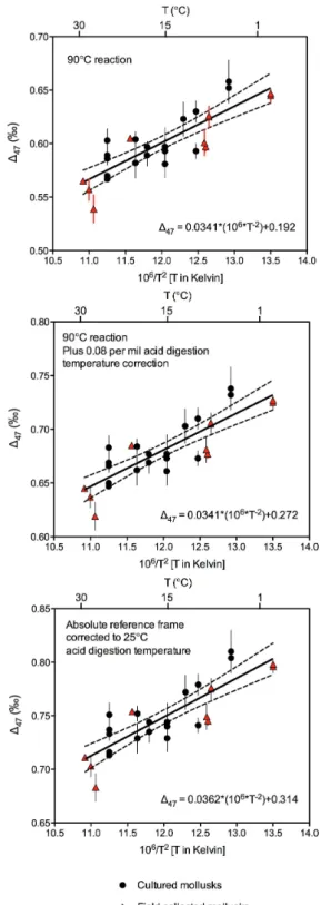
We present data both relative to the stochastic reference frame (to aid comparison with previously published data) and in the recently proposed absolute reference frame (Tables 1– 6 and S1). The most direct analysis of our data (i.e. involving a minimum of calculations) is the empirical correlation be-tween known growth temperature and147 value of bivalve carbonate relative to the stochastic reference frame, using a 90◦C phosphoric acid digestion reaction (Fig. 2; Table 3). This is the temperature that is now standardly used on our au-tomated online sample reaction and gas purification systems (Passey et al., 2010). We then applied the empirically deter-mined acid digestion correction of 0.08 ‰ to derive data rel-ative to the stochastic distribution that could be compared to previously published data collected on CO2produced by di-gesting carbonates in phosphoric acid at 25◦C (Fig. 2). Lin-ear regressions through each dataset are presented in Fig. 2, and are tabulated with calculated uncertainties and alongside previously published regressions in Table 4.
Individual bivalve samples generally conform reasonably well to the temperature relationship defined by the total pop-ulation of bivalve data. However a small number of sam-ples, for example the specimen ofZygochlamys patagonica, show a significant departure from this relationship (i.e. fall outside the 95 % confidence intervals of the linear regres-sion; Fig. 2). This appears to represent a unique property of the sample (possibly a “vital effect”) on147 rather than an imprecise measurement as the result is confirmed by analy-sis of CO2extracted from this specimen 6 times (Table 2). The Levitus atlas of ocean temperatures also calls for a mi-nor difference in mean annual temperature (∼8◦C) versus warm summer month (∼9◦C) temperature at the location and water depth on the Patagonian shelf where this sample was recovered from. Therefore if the database is correct, then
Fig. 2.Bivalve147calibration data. The top panel shows a linear regression with
95 % confidence intervals through147measurements made on both cultured (circles)
and field collected (triangles) mollusks grown at different temperatures. Shells were re-acted with phosphoric acid heated to 90◦C to produce analyte CO
2. These data are
rel-ative to the stochastic distribution as described previously (Huntington et al., 2009) and do not have the empirically derived acid digestion correction of 0.08 ‰ added (Passey et al., 2010), which is used to compare data to that derived from a 25◦C acid digestion reaction. The middle panel is the data with this correction. The bottom panel is bivalve calibration data with the acid digestion correction, then converted into the absolute ref-erence frame (Dennis et al., 2011) using a secondary transfer function. Equations for the relationship between measured147and bivalve growth temperature are given in
Table 1.Effect of oxidative sample cleaning on mollusk stable isotope data.
Taxa Sample Growth Sample Mineralogy2 Total δ13C δ18O 147 147
ID Temperature1 Treatment Number of ‰ ‰ ‰ ‰
(◦C) Analyses3 V-PDB V-PDB (SD)4 (ARF)5
Crassostrea virginica JR-126 25 None C 6 −0.5 −1.7 0.650±0.005 0.716±0.005
Crassostrea virginica JR-126 25 3 % H2O2 C 6 −0.4 −1.2 0.651±0.012 0.716±0.012
Mya arenaria JR-131 25 None A≫C 3 −1.0 −3.3 0.648±0.005 0.714±0.005
Mya arenaria JR-131 25 3 % H2O2 A≫C 3 −1.0 −3.3 0.644±0.002 0.709±0.002
1Cultured specimen growth temperature is accurate to within 0.5◦C on average (see methods). For field collected specimens temperatures correspond to average temperatures for the three warmest months (assumed to be the predominant growing season), it is assumed that there is a 1◦C error in growth temperatures on average. Ocean temperatures determined from the Levitus database. All temperatures are rounded to the nearest integer.
2C, calcite; A, aragonite.≫refers to a mixed mineralogy with one mineral predominating. For the purpose of isotope calculations the dominant mineralogy is used. 3Represents the number of distinct extractions of CO
2from a sample, which are then purified and analyzed.
4Relative to the stochastic distribution. Also referred to as data in the Caltech intralaboratory reference frame. Includes the acid digestion correction of 0.08.±. Values are 1 s.e. 5Values given on the absolute reference frame.
incorrect attribution of the season of growth to the summer months in Fig. 2 does not seem a likely explanation (Levitus and Boyer, 1994). Additional work on specific taxa will be needed to confirm this observation. Amongst the most sig-nificant departures from previous calibration lines are those from both calcitic and aragonitic specimens forming in the coldest environments, near-freezing shallow marine waters of the Ross Sea off Antarctica that do not reach temperatures significantly above 0◦C all year.
The R2 value of our bivalve mollusk calibration line is 0.7258 (Table 4) using data on the absolute reference frame, and the standard deviation of the residuals (SDR) is 0.017 ‰. This suggests that there is somewhat larger vari-ability in bivalve147 data compared to other biogenic cal-ibration datasets. For example the linear regression through the foraminifera calibration of Tripati et al. (2010) has anR2
value of 0.8998 and a SDR of 0.014 ‰, and for the study of corals by Thiagarajan et al. (2011) theR2 value is 0.8703 with a SDR of 0.015 ‰ (Tripati et al., 2010; Thiagarajan et al., 2011). It is possible that this reflects very subtle biolog-ical or mineralogbiolog-ical effects on bivalve147 data, although, as we describe below, we cannot resolve these effects in our dataset.
In the case of field collected bivalves in the figures and regression analysis presented we assumed that preferential growth occurred in the three warmest summer months. How-ever we accept that many taxa do also grow at other times of the year and so in order to assess the impact of our assump-tion on the resulting regression lines through147versus tem-perature data we also created a regression line using mean an-nual water temperatures (data not shown) for field collected specimens. The slope of a linear regression line through all bivalve data including field collected specimens assumed to reflect mean annual temperature (rather than warm month av-erage temperatures as in figures and tables) is 0.0350 on the absolute reference frame. This compares to a slope of 0.0362 assuming the warm month average temperature is the pre-dominant growing season for field collected bivalve shells
(Table 4). These slopes are not significantly different in an analysis of covariance (ANCOVA) test (p=0.68). There-fore we conclude that our assumptions over the predominant growing season for bivalve mollusks do not significantly im-pact the slope of the linear regression lines presented here.
3.3 Comparison of bivalve147calibration with other
theoretical and empirical calibrations
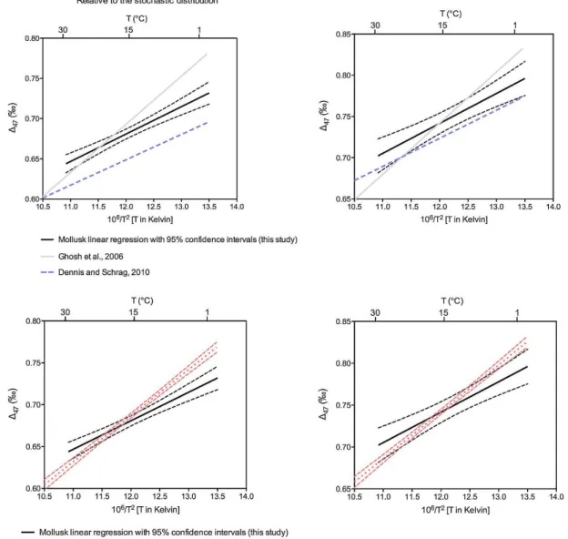
A linear regression through the plot of 1/T versus147 val-ues for our measurements from bivalves produces a signifi-cantly shallower slope than a regression through previously published calibration materials analyzed in our laboratory (Fig. 3). Previous publications did not use the same software or approaches for calculating linear regressions (e.g., Ghosh et al., 2006; and Huntington et al., 2009). Therefore in or-der to compare regressions precisely, as in Figs. 3 and 4, we recalculate all linear regressions using GraphPad Prism soft-ware (Zar, 1984) and it is these values that are presented in Table 4. In practice however these different methods do not yield slopes and intercepts that are markedly different; for ex-ample the linear regression presented by Ghosh et al. (2006) yielded a slope of 0.592, whereas using the software utilized here we yield a slope of 0.598. Linear regressions presented here do not take into account errors in carbonate formation temperatures or isotope measurements; in this dataset these tend to be quite similar on average and do not significantly impact the slope of the regression (data not shown).
Table 2.Average stable isotope data for all mollusk samples grown at seawater in equilibrium with present daypCO2.
Taxa Growth Location Mineralogy2 Number Total 147 147
Temperature1 Individuals Number of ‰ ‰
(◦C) Analysed Analyses3 (SD)4 (ARF)5
Cultured Specimens
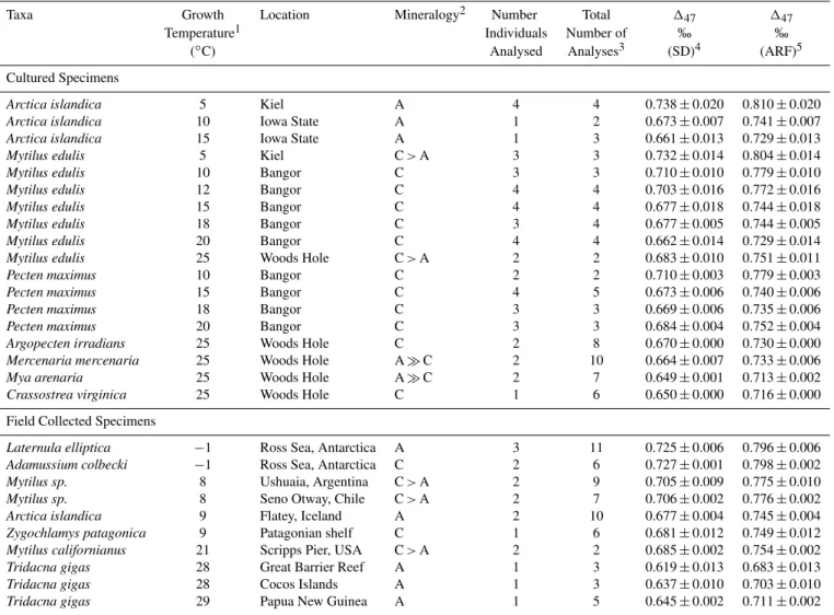
Arctica islandica 5 Kiel A 4 4 0.738±0.020 0.810±0.020
Arctica islandica 10 Iowa State A 1 2 0.673±0.007 0.741±0.007
Arctica islandica 15 Iowa State A 1 3 0.661±0.013 0.729±0.013
Mytilus edulis 5 Kiel C>A 3 3 0.732±0.014 0.804±0.014
Mytilus edulis 10 Bangor C 3 3 0.710±0.010 0.779±0.010
Mytilus edulis 12 Bangor C 4 4 0.703±0.016 0.772±0.016
Mytilus edulis 15 Bangor C 4 4 0.677±0.018 0.744±0.018
Mytilus edulis 18 Bangor C 3 4 0.677±0.005 0.744±0.005
Mytilus edulis 20 Bangor C 4 4 0.662±0.014 0.729±0.014
Mytilus edulis 25 Woods Hole C>A 2 2 0.683±0.010 0.751±0.011
Pecten maximus 10 Bangor C 2 2 0.710±0.003 0.779±0.003
Pecten maximus 15 Bangor C 4 5 0.673±0.006 0.740±0.006
Pecten maximus 18 Bangor C 3 3 0.669±0.006 0.735±0.006
Pecten maximus 20 Bangor C 3 3 0.684±0.004 0.752±0.004
Argopecten irradians 25 Woods Hole C 2 8 0.670±0.000 0.730±0.000
Mercenaria mercenaria 25 Woods Hole A≫C 2 10 0.664±0.007 0.733±0.006
Mya arenaria 25 Woods Hole A≫C 2 7 0.649±0.001 0.713±0.002
Crassostrea virginica 25 Woods Hole C 1 6 0.650±0.000 0.716±0.000
Field Collected Specimens
Laternula elliptica −1 Ross Sea, Antarctica A 3 11 0.725±0.006 0.796±0.006
Adamussium colbecki −1 Ross Sea, Antarctica C 2 6 0.727±0.001 0.798±0.002
Mytilus sp. 8 Ushuaia, Argentina C>A 2 9 0.705±0.009 0.775±0.010
Mytilus sp. 8 Seno Otway, Chile C>A 2 7 0.706±0.002 0.776±0.002
Arctica islandica 9 Flatey, Iceland A 2 10 0.677±0.004 0.745±0.004
Zygochlamys patagonica 9 Patagonian shelf C 1 6 0.681±0.012 0.749±0.012
Mytilus californianus 21 Scripps Pier, USA C>A 2 2 0.685±0.002 0.754±0.002
Tridacna gigas 28 Great Barrier Reef A 1 3 0.619±0.013 0.683±0.013
Tridacna gigas 28 Cocos Islands A 1 3 0.637±0.010 0.703±0.010
Tridacna gigas 29 Papua New Guinea A 1 5 0.645±0.002 0.711±0.002
1Cultured specimen growth temperature is accurate to within 0.5◦
C on average (see methods). For field collected specimens temperatures correspond to average temperatures for the three warmest months (assumed to be the predominant growing season), it is assumed that there is a 1◦C error in growth temperatures on average. Ocean temperatures determined from the Levitus database. All temperatures are rounded to the nearest integer.
2C, calcite; A, aragonite.≫refers to a mixed mineralogy with one mineral predominating. For the purpose of isotope calculations the dominant mineralogy is used. 3Represents the number of distinct extractions of CO
2from all samples, which are then purified and analyzed.
4Relative to the stochastic distribution. Also referred to as data in the Caltech intralaboratory reference frame. Includes the acid digestion correction of 0.08.±. Values are 1 s.e. 5Values given on the absolute reference frame.
indistinguishable, there could be an offset in the absolute val-ues of the two. We also note that the apparently higher vari-ability in the bivalve mollusk dataset compared to other bio-genic calibration datasets is taken into account by the statis-tical analysis of slopes presented in Table 5 and so this vari-ability itself cannot explain the statistically significant differ-ences in slopes we observe.
In order to consider whether the slope of the bivalve linear regression could be significantly effected by a few anomalous datapoints we tested the effect of excluding the five speci-mens recovered from the coldest temperatures from Antarc-tica (Laternula ellipticaandAdamussium colbecki)that are also amongst the most different from the calibration line of Ghosh et al. (2006), yielding147values of 0.72–0.74 ‰
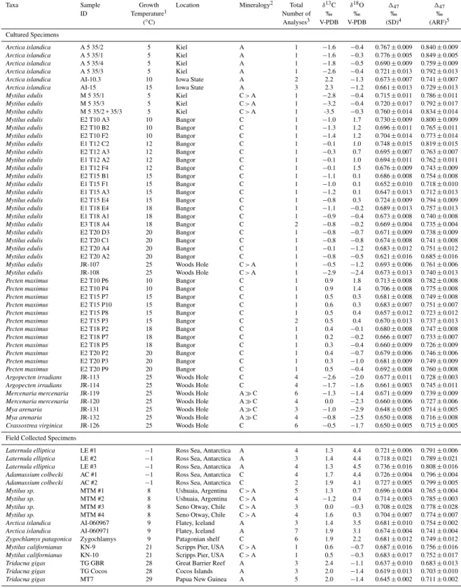
Table 3.Stable isotope data for individual mollusk specimens grown at ambient carbonate saturation state and with no cleaning.
Taxa Sample Growth Location Mineralogy2 Total δ13C δ18O 1
47 147
ID Temperature1 Number of ‰ ‰ ‰ ‰
(◦C) Analyses3 V-PDB V-PDB (SD)4 (ARF)5
Cultured Specimens
Arctica islandica A 5 35/2 5 Kiel A 1 −1.6 −0.4 0.767±0.009 0.840±0.009
Arctica islandica A 5 35/1 5 Kiel A 1 −1.6 −0.3 0.776±0.005 0.849±0.005
Arctica islandica A 5 35/4 5 Kiel A 1 −1.8 −0.5 0.690±0.009 0.759±0.009
Arctica islandica A 5 35/3 5 Kiel A 1 −2.6 −0.4 0.721±0.013 0.792±0.013
Arctica islandica AI-10.3 10 Iowa State A 2 2.2 −1.3 0.673±0.007 0.741±0.007
Arctica islandica AI-15 15 Iowa State A 3 2.3 −1.2 0.661±0.013 0.729±0.013
Mytilus edulis M 5 35/1 5 Kiel C>A 1 −2.8 −0.4 0.715±0.011 0.786±0.011
Mytilus edulis M 5 35/3 5 Kiel C>A 1 −3.2 −0.4 0.720±0.017 0.792±0.017
Mytilus edulis M 5 35/2 + 35/3 5 Kiel C>A 1 -3.5 −0.3 0.760±0.014 0.834±0.014
Mytilus edulis E2 T10 A3 10 Bangor C 1 −1.0 1.7 0.730±0.009 0.800±0.009
Mytilus edulis E2 T10 B2 10 Bangor C 1 −1.3 1.2 0.696±0.011 0.765±0.011
Mytilus edulis E2 T10 F2 10 Bangor C 1 −1.4 1.2 0.704±0.014 0.773±0.014
Mytilus edulis E1 T12 C2 12 Bangor C 1 −0.1 1.0 0.748±0.015 0.819±0.015
Mytilus edulis E2 T12 A3 12 Bangor C 1 −0.3 0.7 0.695±0.007 0.763±0.007
Mytilus edulis E1 T12 A2 12 Bangor C 1 −0.1 1.0 0.694±0.011 0.762±0.011
Mytilus edulis E1 T12 F4 12 Bangor C 1 −0.1 1.5 0.676±0.009 0.743±0.009
Mytilus edulis E2 T15 B1 15 Bangor C 1 −1.1 0.1 0.686±0.008 0.754±0.008
Mytilus edulis E1 T15 F1 15 Bangor C 1 −1.0 0.1 0.652±0.010 0.718±0.010
Mytilus edulis E1 T15 A3 15 Bangor C 1 −1.2 0.1 0.647±0.013 0.712±0.013
Mytilus edulis E2 T15 E4 15 Bangor C 1 −0.8 0.3 0.724±0.009 0.794±0.009
Mytilus edulis E1 T18 E4 18 Bangor C 1 −1.1 −0.2 0.689±0.013 0.757±0.013
Mytilus edulis E1 T18 A1 18 Bangor C 1 −0.9 −0.4 0.673±0.008 0.740±0.008
Mytilus edulis E3 T18 A4 18 Bangor C 2 −0.8 −0.2 0.669±0.004 0.735±0.004
Mytilus edulis E2 T20 D3 20 Bangor C 1 −0.8 −0.7 0.671±0.009 0.738±0.009
Mytilus edulis E2 T20 C1 20 Bangor C 1 −0.8 −0.8 0.674±0.008 0.741±0.008
Mytilus edulis E2 T20 A4 20 Bangor C 1 −0.1 −1.2 0.683±0.012 0.751±0.012
Mytilus edulis E2 T20 A2 20 Bangor C 1 −0.8 −0.5 0.621±0.016 0.685±0.016
Mytilus edulis JR-107 25 Woods Hole C>A 1 −0.5 −1.2 0.693±0.006 0.761±0.006
Mytilus edulis JR-108 25 Woods Hole C>A 1 −2.9 −2.4 0.673±0.013 0.740±0.013
Pecten maximus E2 T10 P6 10 Bangor C 1 0.9 1.8 0.713±0.008 0.782±0.008
Pecten maximus E2 T10 P4 10 Bangor C 1 0.9 1.4 0.706±0.008 0.775±0.008
Pecten maximus E2 T15 P7 15 Bangor C 1 0.5 0.3 0.681±0.008 0.749±0.008
Pecten maximus E2 T15 P10 15 Bangor C 1 0.6 0.3 0.683±0.007 0.751±0.007
Pecten maximus E2 T15 P8 15 Bangor C 1 0.5 0.4 0.657±0.012 0.723±0.012
Pecten maximus E2 T15 P3 15 Bangor C 2 0.5 0.4 0.670±0.013 0.737±0.013
Pecten maximus E2 T18 P2 18 Bangor C 1 0.4 −0.1 0.680±0.008 0.747±0.008
Pecten maximus E2 T18 P7 18 Bangor C 1 0.2 −0.2 0.666±0.007 0.733±0.007
Pecten maximus E2 T18 P5 18 Bangor C 1 0.3 −0.4 0.660±0.009 0.726±0.009
Pecten maximus E2 T20 P2 20 Bangor C 1 0.4 −0.7 0.679±0.006 0.746±0.006
Pecten maximus E2 T20 P3 20 Bangor C 1 0.3 −1.0 0.681±0.009 0.749±0.009
Pecten maximus E2 T20 P9 20 Bangor C 1 0.5 −0.4 0.692±0.008 0.760±0.008
Argopecten irradians JR-113 25 Woods Hole C 4 −2.6 −2.0 0.677±0.011 0.728±0.003
Argopecten irradians JR-114 25 Woods Hole C 4 −1.7 −1.6 0.661±0.003 0.745±0.011
Mercenaria mercenaria JR-119 25 Woods Hole A≫C 6 −1.3 −1.4 0.671±0.009 0.739±0.009
Mercenaria mercenaria JR-120 25 Woods Hole A≫C 4 0.0 −2.3 0.660±0.006 0.727±0.006
Mya arenaria JR-131 25 Woods Hole A≫C 3 −1.0 −2.9 0.648±0.005 0.714±0.005
Mya arenaria JR-132 25 Woods Hole A≫C 4 −0.8 −2.5 0.650±0.008 0.716±0.008
Crassostrea virginica JR-126 25 Woods Hole C 6 −0.5 −1.7 0.650±0.005 0.715±0.005
Field Collected Specimens
Laternula elliptica LE #1 −1 Ross Sea, Antarctica A 4 1.3 4.4 0.721±0.006 0.791±0.006
Laternula elliptica LE #2 −1 Ross Sea, Antarctica A 3 1.4 4.4 0.718±0.021 0.789±0.021
Laternula elliptica LE #3 −1 Ross Sea, Antarctica A 4 1.3 4.5 0.736±0.016 0.808±0.016
Adamussium colbecki AC #1 −1 Ross Sea, Antarctica C 4 1.7 4.4 0.726±0.004 0.796±0.004
Adamussium colbecki AC #2 −1 Ross Sea, Antarctica C 2 1.9 4.1 0.727±0.005 0.799±0.005
Mytilus sp. MTM #1 8 Ushuaia, Argentina C>A 5 1.3 0.7 0.696±0.004 0.765±0.004
Mytilus sp. MTM #2 8 Ushuaia, Argentina C>A 4 −1.2 0.4 0.714±0.003 0.785±0.003
Mytilus sp. MTM #3 8 Seno Otway, Chile C>A 3 0.0 −0.3 0.708±0.028 0.778±0.028
Mytilus sp. MTM #4 8 Seno Otway, Chile C>A 4 1.6 0.3 0.704±0.007 0.774±0.007
Arctica islandica AI-060967 9 Flatey, Iceland A 3 1.4 3.5 0.681±0.010 0.754±0.002
Arctica islandica AI-060971 9 Flatey, Iceland A 7 1.9 3.1 0.674±0.004 0.741±0.004
Zygochlamys patagonica Zygochlamys 9 Patagonian shelf C 6 1.9 2.2 0.681±0.012 0.749±0.012
Mytilus californianus KN-9 21 Scripps Pier, USA C>A 1 0.6 −0.7 0.687±0.016 0.756±0.016
Mytilus californianus KN-10 21 Scripps Pier, USA C>A 1 0.5 −0.3 0.683±0.017 0.752±0.017
Tridacna gigas TG GBR 28 Great Barrier Reef A 3 2.4 −1.1 0.637±0.010 0.683±0.013
Tridacna gigas TG Cocos 28 Cocos Islands A 3 2.0 −1.4 0.619±0.013 0.703±0.010
Tridacna gigas MT7 29 Papua New Guinea A 5 2.0 −1.4 0.645±0.002 0.711±0.002
1Cultured specimen growth temperature is accurate to within 0.5◦C on average (see methods). For field collected specimens temperatures correspond to average temperatures for the three warmest months (assumed to be the predominant growing season), it is assumed that there is a 1◦C error in growth temperatures on average. Ocean temperatures determined from the Levitus database. All temperatures are rounded to the nearest integer.
2C, calcite; A, aragonite.≫refers to a mixed mineralogy with one mineral predominating. For the purpose of isotope calculations the dominant mineralogy
is used.
3Represents the number of distinct extractions of CO
2from a sample, which are then purified and analyzed.
4Relative to the stochastic distribution. Also referred to as data in the Caltech intralaboratory reference frame. Includes the acid digestion correction of
0.08.±. Values are 1 s.e.
Fig. 3.Comparison of bivalve147measurements to previously published calibration data. Here we compare the linear regressions through
our mollusk data shown in Fig. 2 to published calibration lines, relative to both the stochastic distribution (left panels) and the absolute reference frame (right panels). In all cases a correction of 0.08 ‰ was made to compare mollusk data to older data collected in our laboratory using 25◦C acid digestion reactions. Mollusk calibration lines have a clearly shallower slope than the inorganic calcite calibration line of Ghosh et al. (2006) and have a similar slope to the calibration of Dennis and Schrag, but with a slight offset to that calibration (Dennis and Schrag, 2010). The mollusk calibration line is also significantly shallower than the linear regression through the compilation of other published materials from our laboratory (bottom panels), with previously published data plotted in this graph given in Table S1.
specimens from Antarctica from the mollusk dataset does yield a steeper slope (Table 4) of 0.0402±0.0050 (1 s.e.) on the absolute reference frame, however it does not change the results of our statistical analysis (Table 5) showing that the bivalve mollusk calibration dataset is has a significantly different slope to the previously published biogenic compi-lation produced in our laboratory and the inorganic calcite calibration of Ghosh et al. (2006).
Whilst it is useful to examine the effect of excluding these samples on the regression line, it is also important to note that at present we do not have a good reason to exclude
these Antarctic specimens from the regression analysis in this way. There is some rationale for supposing that carbon-ates that form at low temperatures could be more prone to record kinetic isotope effects, as described above, however previously published studies onL. ellipticaandA. colbecki
from Antarctica report that their measured δ18O are close to their expected equilibrium values (Barrera et al., 1994, 1990). Whilst we cannot rule out disequilibrium effects in
regard the regression line through all our mollusk data as the most robust calibration.
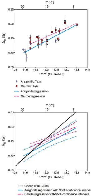
3.4 Calcite versus aragonite
Theoretical calculations predict that there would be an off-set between 147 values derived from calcite compared to aragonite (Schauble et al., 2006; Guo et al., 2009). How-ever measurements from foraminifera and corals have not resolved any mineralogical effect (Tripati et al., 2010; Thi-agarajan et al., 2011). In our mollusk dataset there is a slight offset between the slopes of regression lines between calcitic and aragonitic mollusks (Fig. 4), however the offset is in the opposite direction to that predicted from theory (Schauble et al., 2006; Guo et al., 2009). The slopes of linear regressions through the temperature-147 data for calcitic and aragonitic taxa (Fig. 4) were not significantly different (p=0.520). If a difference between calcitic and aragonitic mollusks ex-ists, then it is not easily resolvable. In some cases bivalves that precipitate shells with mixed mineralogy were selec-tively sampled to only acquire the calcite phase, such as the
M. edulisspecimens grown at Bangor University (Freitas et al., 2008). However, in other cases this distinction was not made and both mineralogies were sampled, as detailed in Table 4. For the calcite versus aragonite comparison sam-ples with mixed mineralogy were excluded. When compar-ing the regression lines through the aragonite data to other calibrations (Table 5) it is worth noting that there does not appear to be enough data to statistically determine which of the two different inorganic calcite calibration lines (Ghosh et al., 2006; Dennis and Schrag, 2010) the aragonitic mollusk data fits best with. Therefore it remains possible that the lack of a mineralogical difference in our study could be further resolved in the future with larger datasets.
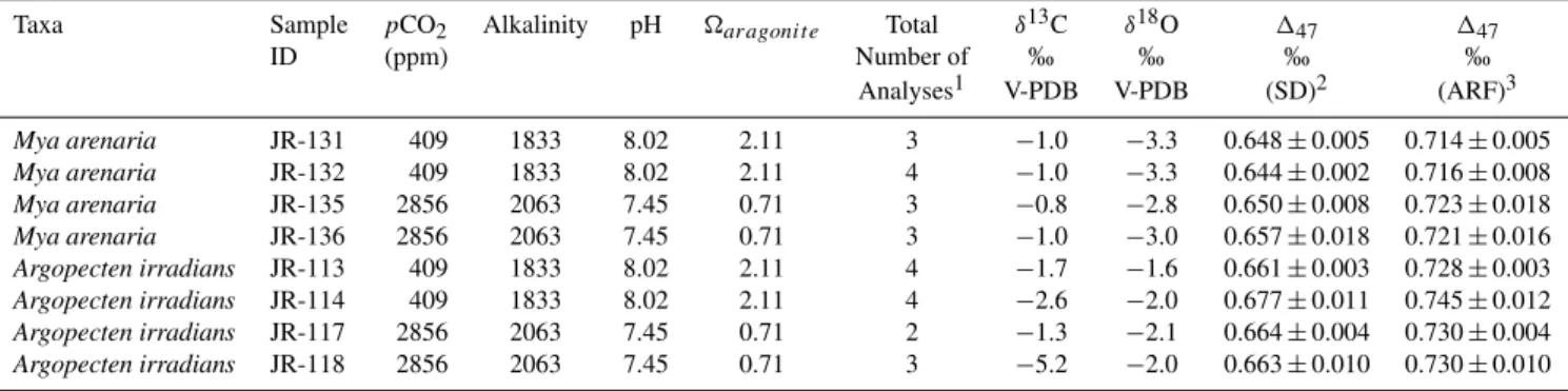
3.5 The influence of seawater carbonate saturation state on bivalve stable isotopes
In a number of biogenic carbonates it has been suggested that changes in solution pH can influence carbonateδ18O (Spero et al., 1997; Rollion-Bard et al., 2003; Adkins et al., 2003). The effect of changing solution pH and carbonate chemistry on13C–18O bond abundance in carbonate minerals has not been explicitly investigated. Here we analyzed specimens of
Mya arenaria, andArgopecten irradiansthat were cultured at 25◦C and with CO2bubbled into the aquarium at either 409 ppm or 2856 ppm producing seawater that was either su-persaturated or undersaturated with respect to aragonite (Ries et al., 2009).M. arenariapredominantly precipitates arag-onite, whilstA. irradiansprecipitates low-Mg calcite. Both species showed a reduction in calcification in undersaturated seawater, but care was taken to only sample new growth in each case (Ries et al., 2009). In both cases no significant ef-fects on δ18O and 147 values were observed in carbonate
Fig. 4.Comparison of bivalve147 data derived from calcitic and
aragonitic taxa. The top panel shows data split between calcitic (squares) and aragonitic (circles) mollusks, with a linear regression through each. Here cultured and field collected samples are not dis-tinguished in the figure. The bottom panel shows linear regressions with 95 % confidence intervals. There is an offset between the re-gressions between calcite and aragonite, but it is not statistically significant.
that was formed by specimens cultured in seawater undersat-urated with respect to aragonite (Table 6).
4 Discussion
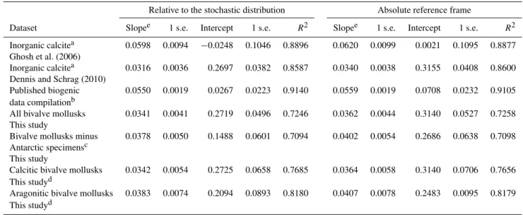
Table 4.Slopes and intercepts of linear regressions through147and temperature data for samples with known growth temperatures.
Relative to the stochastic distribution Absolute reference frame
Dataset Slopee 1 s.e. Intercept 1 s.e. R2 Slopee 1 s.e. Intercept 1 s.e. R2
Inorganic calcitea 0.0598 0.0094 −0.0248 0.1046 0.8896 0.0620 0.0099 0.0021 0.1095 0.8877 Ghosh et al. (2006)
Inorganic calcitea 0.0316 0.0036 0.2697 0.0382 0.8587 0.0340 0.0038 0.3155 0.0408 0.8600 Dennis and Schrag (2010)
Published biogenic 0.0550 0.0019 0.0267 0.0223 0.9140 0.0559 0.0019 0.0708 0.0232 0.9105 data compilationb
All bivalve mollusks 0.0341 0.0041 0.2719 0.0496 0.7246 0.0362 0.0044 0.3140 0.0527 0.7258 This study
Bivalve mollusks minus 0.0378 0.0050 0.1488 0.0601 0.7094 0.0402 0.0054 0.2686 0.0638 0.7098 Antarctic specimensc
This study
Calcitic bivalve mollusks 0.0342 0.0054 0.2725 0.0658 0.7685 0.0364 0.0058 0.3140 0.0706 0.7656 This studyd
Aragonitic bivalve mollusks 0.0383 0.0074 0.2094 0.0893 0.8180 0.0407 0.0078 0.2483 0.0095 0.8179 This studyd
aSee Table S1 for the data used for these regression line calculations.
bIncludes coral data from Ghosh et al., 2006 (but excludes Red SeaPorites), and data from Ghosh et al. (2007), Came et al. (2007), Tripati et al. (2010), Eagle et al. (2010),
and Thiagarajan et al. (2011). See Table S1 for values for these data.
cExcluding data from the five individuals ofLaternula ellipticaandAdamussium colbecki(which are Antarctic specimens from the coldest environments sampled in this study)
as a means for determining whether the calibration slope could be significantly influenced by these samples alone.
dExcluding specimens with mixed mineralogy.
eLinear regressions through previously published data are all recalculated here using GraphPad Prism software (Zar, 1984) so that they are directly comparable to the new
mollusk data presented here, and as a result may have slight differences from the slopes and intercepts given in original publications at the third or fourth decimal place. All regressions are on data that include an acid digestion temperature correction where appropriate (Passey et al., 2010). Errors are given as 1 s.e.
Table 5.ANCOVApvalues derived by comparing linear regressions through the dataset generated in this study to previously published data.
Dataseta Inorganic calcite Inorganic calcite Published biogenic data Ghosh et al. (2006) Dennis and Schrag (2010) compilationd
All bivalve mollusks p=0.0035 (Y) p=0.7020 (N) p <0.0001 (Y) This study
Bivalve mollusks minus p=0.0139 (Y) p=0.5453 (N) p=0.0006 (Y) Antarctic speciesb
This study
Calcitic bivalve mollusks p=0.0196 (Y) p=0.9354 (N) p=0.0013 (Y) This studyc
Aragonitic bivalve mollusks p=0.1274 (N) p=0.4664 (N) p=0.0126 (Y) This studyc
aLinear regression lines through different subsets of our mollusk1
47calibration dataset in the first column are statistically compared to using
ANCOVA tests (Zar, 1984) to linear regressions through other previously published calibration studies datasets. Calculations are done with values on the absolute reference frame (ARF). The table displays the ANCOVApvalue and whether the two slopes being compared are statistically different; (Y) = Yes, (N) = No. In this case we consider apvalue<0.05 as indicating statistically significant differences between the two slopes.
bExcluding the five specimens ofLaternula ellipticaandAdamussium colbecki(which are specimens from the coldest Antarctic
environments) as a means for determining whether the calibration slope could be significantly influenced by these samples alone.
cExcluding specimens with mixed mineralogy.
dIncludes coral data from Ghosh et al. (2006) (but excludes Red SeaPorites), and data from Ghosh et al. (2007), Came et al. (2007), Tripati et
al. (2010), Eagle et al. (2010), and Thiagarajan et al. (2011). See Table S1 for values for these data.
mollusks. We also show that changing solution pH and car-bonate chemistry should not be a confounding factor in the interpretation of bivalve based147 or δ18O measurements, at least in the taxa studied, and that there is no significant mineralogical difference between calcite and aragonite. The errors in slope and intercepts for linear regression lines given
Table 6.Stable isotope data for individual cultured mollusk specimens grown at ambient carbonate saturation state and undersaturated conditions.
Taxa Sample pCO2 Alkalinity pH aragonit e Total δ13C δ18O 147 147
ID (ppm) Number of ‰ ‰ ‰ ‰
Analyses1 V-PDB V-PDB (SD)2 (ARF)3
Mya arenaria JR-131 409 1833 8.02 2.11 3 −1.0 −3.3 0.648±0.005 0.714±0.005
Mya arenaria JR-132 409 1833 8.02 2.11 4 −1.0 −3.3 0.644±0.002 0.716±0.008
Mya arenaria JR-135 2856 2063 7.45 0.71 3 −0.8 −2.8 0.650±0.008 0.723±0.018
Mya arenaria JR-136 2856 2063 7.45 0.71 3 −1.0 −3.0 0.657±0.018 0.721±0.016
Argopecten irradians JR-113 409 1833 8.02 2.11 4 −1.7 −1.6 0.661±0.003 0.728±0.003
Argopecten irradians JR-114 409 1833 8.02 2.11 4 −2.6 −2.0 0.677±0.011 0.745±0.012
Argopecten irradians JR-117 2856 2063 7.45 0.71 2 −1.3 −2.1 0.664±0.004 0.730±0.004
Argopecten irradians JR-118 2856 2063 7.45 0.71 3 −5.2 −2.0 0.663±0.010 0.730±0.010
Culture conditions and seawater chemistry measurements are from Ries et al. (2009).
1Represents the number of distinct extractions of CO
2from all samples, which are then purified and analyzed.
2Relative to the stochastic distribution only. Also referred to as data in the Caltech intralaboratory reference frame. Includes the acid digestion correction of 0.08.±. Values are
1 s.e.
3Values given on the absolute reference frame.
aragonite=[Ca2+][CO23−] /Ksp, whereKspis the stoichiometric solubility product of aragonite.aragonitewas calculated as described in Ries et al. (2009).
laboratory due to having fewer datapoints. However we have shown statistically that the uncertainties in these calibration lines cannot alone explain the difference between our bivalve mollusk calibration line and other data produced in our labo-ratory, which (i) highlights that empirical calibrations of the carbonate clumped isotope paleothermometer are vital for each type of material and experimental setup, and (ii) sug-gests that initial papers showing close similarity of some bio-genic materials to the inorganic calcite calibration of Ghosh et al. (2006; Eagle et al., 2010; Tripati et al., 2010; Thiagara-jan et al., 2011) should not be assumed to hold in all cases. We also note that after this manuscript was published as a dis-cussion paper, another study of brachiopods and mollusks in a different laboratory also reported a similarly shallow slope (Henkes et al., 2013), although as these measurements were conducted using a very similar methodology to that used in our study the similarity between our calibration slopes does not entirely resolve the possible methodological differences between calibration studies described below.
There are two possible explanations that are immediately apparent for the differences between calibration lines gener-ated from different materials in our laboratory. First, the bi-valve mollusk data presented here was obtained using the au-tomated online sample reaction system described in Passey et al., 2010, whereas the in-depth calibration studies of corals, foraminifera and coccoliths were conducted using offline reactions with cryogenic and gas chromatography cleanup steps performed manually (Passey et al., 2010; Tripati et al., 2010; Thiagarajan et al., 2011). The calibration study on bioapatite (Eagle et al., 2010) was conducted on the auto-mated system, but it did not examine specimens grown at temperatures lower than∼24◦C and so would not necessar-ily have resolved a difference in slope that would be most apparent at low temperatures. Therefore we must consider the possibility that an experimental effect, such as
fractiona-tion of gases in either offline or online systems, or an effect due to the differences in acid digestion temperature between the two systems (25◦C for the offline reactions, 90◦C for the automated systems, which is presently addressed using a cor-rection of 0.08 ‰ on the Caltech intralab reference frame) is not being correctly accounted for. Evidence against an ex-perimental artifact from these two sources comes from the broadly comparable results that have been generated in dif-ferent labs that use difdif-ferent systems for purifying CO2gas and different acid digestion temperatures as part of an in-terlaboratory comparison, which included measurements on a cold-water coral standard in four laboratories that consis-tently yielded a147value in the range of 0.78–0.80 ‰ on the absolute reference frame (Dennis et al., 2011). Additionally a number of applied studies using the automated sample prepa-ration system have found that the calibprepa-ration of Ghosh et al. (2006) generally yields plausible results including on modern specimens where we have good controls over growth tem-perature (e.g., Passey et al., 2010; Eagle et al., 2010, 2011, 2013; Finnegan et al., 2011; Csank et al., 2011; and Suarez et al., 2011). Nevertheless most applied studies have focused on samples formed at temperatures of 20◦C or more, and so there is a possibility that experimental differences such as small amounts of gas fractionation or equilibration dur-ing sample gas purification could preferentially affect sam-ples with heavier147values (>0.75 ‰). This is an area that should be explored in the future. Another possibility is that there are variations in acid digestion fractionation factors for samples of different isotopic composition or of different min-eralogy, and whilst the aragonitic cold-water coral did not show this effect (Dennis et al., 2011) it would be useful to check if this is the case in other materials.
biogenic carbonates that could result in “vital effects” on
147. In this scenario the closer match of deep sea corals to the calibration of Ghosh et al. (2006) at cold temperatures ac-tually reflects the expression of a small kinetic isotope effect in all of these materials, one that is not found in mollusks. The data from foraminifera at cold temperatures is relatively sparse, with some samples from the Arctic Ocean showing deviations from the Caltech inorganic calcite calibration and so are analogous to the mollusk data presented here, but other datapoints from specimens from slightly warmer environ-ments fall closer to the calibration of Ghosh et al. (2006), and Tripati et al. (2010). This highlights the relative paucity of data from carbonates forming at low temperatures and this is an obvious area to focus on in future calibration studies.
Bivalve mollusks frequently precipitate their shells close to equilibrium with respect to oxygen isotopes, with maxi-mum deviations typically in the range of 0.5 ‰ (e.g., Horibe and Oba, 1972; Romanek and Grossman, 1989; Grossman and Ku, 1986; Barrera et al., 1994; and Wanamaker et al., 2006). This is in contrast to deep-sea corals, which exhibit nonequilibriumδ18O values of up to 4–5 ‰ in some cases (e.g., Adkins et al. 2003). Therefore we might expect that bivalve mollusk derived147 values may also record close to equilibrium values, unless there is a source of biologi-cal fractionation of 147 in bivalves that has not yet been identified but hypothetically could be linked to mollusk spe-cific mechanisms of biomineralization such as the use of organic templates for carbonate precipitation (Weiner and Dove, 2003; Addadi et al., 2006). If it was the case that mol-lusks are recording close to equilibrium values, the calibra-tion of Ghosh et al. (2006) would have to include a kinetic isotope effect that fortuitously matches “vital effects” in pre-viously published biogenic data from a temperature range of 0–10◦C that falls close to the inorganic calcite values. Fi-nally, we note that even though a mineralogical difference between calcite and aragonite could not be resolved in our dataset it is still possible that very subtle mineralogical ef-fects do exist and these efef-fects contribute to the variability in measured147 values. Larger datasets may be required to constrain this possibility with more certainty.
In conclusion, if the experimental effects described above can be either ruled out or better constrained, we will be able to say more about whether there may be small biological fractionations in147that differ between corals, foraminifera, and bivalves, and why these fractionations are most apparent at cold temperatures.
Supplementary material related to this article is available online at: http://www.biogeosciences.net/10/ 4591/2013/bg-10-4591-2013-supplement.pdf.
Acknowledgements. This work was funded by National Science Foundation grants ARC-1215551 to R. A. Eagle and A. K. Tripati, EAR-1024929 to R. A. Eagle and J. M. Eiler, and EAR-0949191 to A. K. Tripati. A. K. Tripati is also supported by the Hellman Fel-lowship program. We thank Chris Richardson (Bangor University) for provision of the field collected Arctica islandica specimens. Culture of bivalves in Kiel, Germany, was funded by the German Science Foundation (DFG Ei272/21-1, to Anton Eisenhauer) and the European Science Foundation (ESF) Collaborative Research Project CASIOPEIA (04 ECLIM FP08). Determination of bi-valve mineralogy by J. B. Ries was funded by National Science Foundation grant OCE-1031995. ISMAR-CNR Bologna scientific contribution n. 1781.
Edited by: A. Shemesh
References
Addadi, L., Joester, D., Nudelman, F., and Weiner, S.: Mollusk Shell Formation: a Source of New Concepts for Understanding Biomineralization Processes, Chem. Eur. J., 12, 980–987, 2006. Adkins, J. F., Boyle, E. A., Curry, W. B., and Lutringer, A.:
Sta-ble isotopes in deep-sea corals and a new mechanism for “vital effects”, Geochem. Cosmochim. Ac., 67, 1129–1143, 2003. Affek, H. and Eiler, J. M.: Abundance of mass 47 CO2in urban air,
car exhaust, and human breath Geochim. Cosmochim. Ac., 70, 1–12, 2006.
Barrera, E., Tevesz, M. J. S., and Carter, J. G.: Variations in Oxy-gen and Carbon Isotopic Compositions and Microstructure of the Shell ofAdamussium colbecki(Bivalvia), Palaios, 5, 149–159, 1990.
Barrera, E., Tevesz, M. J., Carter, J. G., and McCall, P. L.: Oxygen and Carbon Isotopic Composition and Shell Microstructure of the BivalveLaternula ellipticafrom Antarctica, Palaios, 9, 275– 287, 1994.
Beirne, E. C., Wanamaker, A. D., and Feindel, S. C.: Experimental validation of environmental controls on the delta C-13 of Arc-tica islandica(ocean quahog) shell carbonate, Geochem. Cos-mochim. Ac., 84, 395–409, 2012.
Came, R. E., Eiler, J. M., Veizer, J., Azmy, K., Brand, U., and Wei-dman, C. R.: Coupling of surface temperatures and atmospheric CO2concentrations during the Palaeozoic era, Nature, 449, 198–
201, 2007.
Csank, A. Z., Tripati, A. K., Patterson, W. P., Eagle, R. A., Ry-bczynski, N., Ballantyne, A. P., and Eiler, J. M.: Estimates of Arctic land surface temperatures during the early Pliocene from two novel proxies, Earth Planet. Sci. Lett., 304, 291–299, 2011. Dennis, K. J. and Schrag, D. P.: Clumped isotope thermometry of
carbonatites as an indicator of diagenetic alteration, Geochim. Cosmochim. Ac., 74, 4110–4122, 2010.
Dennis, K. J., Affek, H. P., Passey, B. H., Schrag, D. P., and Eiler, J. M.: Defining an absolute reference frame for “clumped” iso-tope studies of CO2, Geochim. Cosmochim. Ac., 75, 7117–7131, 2011.
Dodd, J. R.: Environmental control of strontium and magnesium in mytilus, Geochim. Cosmochim. Ac., 29, 385–398, 1965. Eagle, R. A., Schauble, E. A., Tripati, A. K., T¨utken, T., Hulbert,
vertebrates from13C-18O bond abundances in bioapatite, P. Natl. Acad. Sci. USA, 107, 10377–10382, 2010.
Eagle, R. A., Tutken, T., Martin, T. S., Tripati, A. K., Fricke, H. C., Connely, M., Cifelli, R. L., and Eiler, J. M.: Dinosaur Body Temperatures Determined from Isotopic (13C-18O) Ordering in Fossil Biominerals, Science, 333, 443–445, 2011.
Eagle, R. A., Risi, C., Mitchell, J. L., Eiler, J. M., Seibt, U., Neelin, J. D., Li, G., and Tripati, A. K.: High regional climate sensitivity over continental China constrained by glacial-recent changes in temperature and the hydrologic cycle, P. Natl. Acad. Sci. USA, 110, 8813–8818, 2013.
Eiler, J. M.: Paleoclimate reconstruction using carbonate clumped isotope thermometry, Quatern. Sci. Rev., 30, 3575–3588, 2011. Eiler, J. M. and Schauble, E.:18O13C16O in Earth’s atmosphere,
Geochim. Cosmochim. Ac., 68, 4767–4777, 2004.
Epstein, S., Buchsbaum, R., Lowenstam, H., and Urey, H. C.: Re-vised carbonate water isotopic temperature scale, Bull. Geol. Soc. Amer., 64, 1315–1326, 1953.
Finnegan, S., Bergmann, K., Eiler, J. M., Jones, D. S., Fike, D. A., Eisenman, I., Hughes, N. C., Tripati, A. K., and Fischer, W. W.: The Magnitude and Duration of Late Ordovician-Early Silurian Glaciation, Science, 331, 903–906, 2011.
Freitas, P. S., Clarke, L. J., Kennedy, H., Richardson, C. A., and Abrantes, F.: Environmental and biological controls on elemen-tal (Mg/Ca, Sr/Ca and Mn/Ca) ratios in shells of the king scallop Pecten maximus, Geochem. Cosmochim. Ac., 70, 5119–5133, 2006.
Freitas, P. S., Clarke, L. J., Kennedy, H. A., and Richardson, C. A.: Inter- and intra-specimen variability masks reliable temperature control on shell Mg/Ca ratios in laboratory- and field-cultured Mytilus edulisandPecten maximus(bivalvia), Biogeosciences, 5, 1245–1258, doi:10.5194/bg-5-1245-2008, 2008.
Freitas, P. S., Clarke, L. J., Kennedy, H., and Richardson, C. A.: Ion microprobe assessment of the heterogeneity of Mg/Ca, Sr/Ca and Mn/Ca ratios in Pecten maximus and Mytilus edulis (bi-valvia) shell calcite precipitated at constant temperature, Biogeo-sciences, 6, 1209–1227, doi:10.5194/bg-6-1209-2009, 2009. Ghosh, P., Adkins, J., Affek, H., Balta, B., Guo, W. F., Schauble, E.
A., Schrag D., and Eiler, J. M.:13C–18O bonds in carbonate min-erals: a new kind of paleothermometer, Geochim. Cosmochim. Ac., 70, 1439–1456, 2006.
Ghosh, P., Eiler, J., Campana, S. E., and Feeney, R. F.: Calibration of the carbonate “clumped isotope” paleothermometer for otoliths, Geochim. Cosmochim. Ac., 71, 2736–2744, 2007.
Gillikin, D. P., Lorrain, A., Navaz, J., Taylor, J. W., Keppens, E., Baeyens, W., and Dehairs, F.: Strong biological controls on Sr/Ca ratios in aragonitic marine bivalve shells, Geochem. Geophys. Geosy., 6, Q05009, doi:10.1029/2004GC000874, 2005. Grossman, E. L., and Ku, T. L.: Oxygen and carbon isotope
fraction-ation in biogenic aragonite - temperature effects, Chem. Geol., 59, 59–74, 1986.
Guo, W., Daeron, M., Niles, P., Genty, D., Kim, S. T., Vonhof, H., Affek, H., Wainer, K., Blamart, D., and Eiler, J.:13C-18O bonds in dissolved inorganic carbon: Implications for carbonate clumped isotope thermometry, Geochem. Cosmochim. Ac., 72, A336, 2008.
Guo, W., Mosenfelder, J. L., Goddard III, W. A., and Eiler, J. M.: Isotopic fractionations associated with phosphoric acid digestion of carbonate minerals: insights from first-principles theoretical
modeling and clumped isotope measurements, Geochim. Cos-mochim. Ac., 73, 7203–7225, 2009.
Heinemann, A., Hiebenthal, C., Fietzke, J., Eisenhauer, A., and Wahl, M.: Disentangling the biological and environmental con-trol of M. edulis shell chemistry, Geochem. Geophys. Geosys., 12, Q03009, doi:10.1029/2010GC003340, 2011.
Henkes, G. A., Passey, B. H., Wanamaker, A. D., Grossman, E. L., Ambrose, W. G., and Carroll, M. L.: Carbonate clumped isotope compositions of modern marine mollusk and brachiopod shells. Geochim. Cosmochim. Ac., 106, 307–325, 2013.
Hiebenthal, C., Philipp, E. R. R., Eisenhauer, A., and Wahl, M.: Interactive effects of temperature and salinity on shell formation and general condition in Baltic SeaMytilus edulisandArctica islandica, Aquat. Biol., 14, 289–298, 2012.
Hill, P. S., Schauble, E. A., and Tripati, A. K.: Theoretical Con-straints on the Effects of pH, Salinity, and Temperature on Clumped Isotope Signatures of Dissolved Inorganic Carbon Species and Precipitating Carbonate Minerals, Geochim. Cos-mochim. Ac., doi:10.1016/j.gca.2013.06.018, 2013.
Horibe, Y. and Oba, T.: Temperature scales of aragonite-water and calcite-water systems, Fossils, 23/24, 69–79, 1972.
Huntington, K. W., Eiler, J. M., Affek, H. P., Guo, W., Bonifacie, M., Yeung, L. Y., Thiagarajan, N., Passey, B., Tripati, A., Da¨eron, M., and Came, R.: Methods and limitations of “clumped” CO2 isotope (Delta47) analysis by gas-source isotope ratio mass spec-trometry, J. Mass Spectrom., 44, 1318–1329, 2009.
Ivany, L. C., Lohmann, K. C., Hasiuk, F., Blake, D. B., Glass, A., Aronson, R. B., and Moody, R. M.: Eocene climate record of a high southern latitude continental shelf: Seymour Island, Antarc-tica, GSA Bulletin, 120, 659–678, 2008.
Johnson, K. S.: Carbon dioxide hydration and dehydration kinetics in seawater, Limnol. Oceanogr., 27, 849–855, 1982.
Keith, M. L., Anderson, G. M., and Eichler, R.: Carbon and oxygen isotopic composition of mollusk shells from marine and fresh-water environments, Geochim. Cosmochim. Ac., 28, 1757–1786, 1964.
Killingley, J. S. and Berger, W. H.: Stable isotopes in a mollusk shell – detection of upwelling events, Science, 205, 186-188, 1979. Kim, S.-T., Mucci, A., and Taylor, B.: Phosphoric acid fractionation
factors for calcite and aragonite between 25 and 75◦C, Chem. Geol., 246, 135–146, 2007.
Klein, R. T., Lohmann, K. C., and Thayer, C. W.: Sr/Ca and13C/12C ratios in skeletal calcite ofMytilus trossulus: Covariation with metabolic rate, salinity, and carbon isotopic composition of sea-water, Geochim. Cosmochim. Ac., 60, 4207–4221, 1996. Levitus, S. and Boyer, T.: World Ocean Atlas 1994:
Tempera-ture, edited by: NESDIS4, N. A., US Department of Commerce, Washington DC, 1994.
Lorens, R. B. and Bender, M. L.: The impact of solution chemistry onMytilus eduliscalcite and aragonite, Geochim. Cosmochim. Ac., 44, 1265–1278, 1980.
McConnaughey, T.:13C and18O isotopic disequilibrium in biolog-ical carbonates. I. Patterns, Geochem. Cosmochim. Ac., 53, 151– 162, 1989.