www.the-cryosphere.net/5/445/2011/ doi:10.5194/tc-5-445-2011
© Author(s) 2011. CC Attribution 3.0 License.
The Cryosphere
In-situ multispectral and bathymetric measurements over a
supraglacial lake in western Greenland using a remotely controlled
watercraft
M. Tedesco1,2and N. Steiner1,2
1The City College of New York, CUNY, NYC, NY, USA 2The Graduate Center, CUNY, NYC, NY, USA
Received: 31 December 2010 – Published in The Cryosphere Discuss.: 7 February 2011 Revised: 17 May 2011 – Accepted: 20 May 2011 – Published: 27 May 2011
Abstract. Supraglacial lakes form from meltwater on the Greenland ice sheet in topographic depressions on the sur-face, affecting both surface and sub-glacial processes. As the reflectance in the visible and near-infrared regions of a column of water is modulated by its height, retrieval tech-niques using spaceborne remote sensing data (e.g. Land-sat, MODIS) have been proposed in the literature for the detection of lakes and estimation of their volume. These techniques require basic assumptions on the spectral prop-erties of the water as well as the bottom of the lake, among other things. In this study, we report results obtained from the analysis of concurrent in-situ multi-spectral and depth measurements collected over a supraglacial lake during early July 2010 in West Greenland (Lake Olivia, 69◦36′35′′N, 49◦29′40′′W) and aim to assess some of the underlying hy-potheses in remote sensing based bathymetric approaches. In particular, we focus our attention on the analysis of the lake bottom albedo and of the water attenuation coefficient. The analysis of in-situ data (collected by means of a remotely controlled boat equipped with a GPS, a sonar and a spectrom-eter) highlights the exponential trend of the water-leaving re-flectance with lake depth. The values of the attenuation fac-tor obtained from in-situ data are compared with those com-puted using approaches proposed in the literature. Also, the values of the lake bottom albedo from in-situ measurements are compared with those obtained from the analysis of re-flectance of shallow waters. Finally, we quantify the error between in-situ measured and satellite-estimated lake depth values for the lake under study.
Correspondence to:M. Tedesco (mtedesco@sci.ccny.cuny.edu)
1 Background and rationale
Supraglacial lakes are pools of meltwater that form during summer in depressions in the ice sheet surface. Monitoring the spatio-temporal variability of such lakes over the Green-land ice sheet (GrIS) can benefit studies concerning ice sheet dynamics (Das et al., 2008; Joughin et al., 1996; Pimentel and Flowers, 2010) and surface features (e.g., L¨uthje et al., 2006) and can help understanding their link with recently observed increased surface melting (Tedesco et al., 2011). Recently, several approaches based on the interpretation of visible and near-infrared satellite data have been proposed for estimating supraglacial lake depth (e.g., Georgiou et al. 2009; Box and Ski, 2007). McMillan et al. (2007) use satel-lite imagery to study the evolution of 292 lakes over an area of 22 000 km2; Sundal et al. (2009) analyze 268 cloud-free Moderate Resolution Imaging Spectroradiometer (MODIS) images; Sneed and Hamilton (2007) estimate the depth of se-lected lakes based on Advanced Spaceborne Thermal Emis-sion and Reflection radiometer (ASTER) atmospherically corrected reflectance values.
the analysis to reduce the impact of cloud cover (Box and Ski, 2007). For those pixels where a lake is detected, lake depth is then estimated using a regression formula obtained from the fitting of in-situ lake depth measurements to satel-lite reflectance values. The main advantage of the method proposed by Box and Ski (2007) lies in its low computa-tional cost. However, results are based on a limited number of measurements over selected lakes and the extension of the method to other areas would require further validation and assesment. A physically-based retrieval has been proposed by Sneed and Hamilton (2007). This is the approach that will be used in this study as it offers the opportunity to evaluate some of the theoretical assumptions adopted in the retrieval scheme. The approach is briefly described and discussed in the following.
For retrieval purposes, the following hypotheses on the bottom albedoAdand on the attenuation factorgare made: (hyp. 1) in the absence of actual measurements the value of Ad is assumed to be uniform and (hyp. 2) Ad is esti-mated from reflectance values of shallow waters along the lake edge (e.g., Sneed and Hamilton, 2007); the attenua-tion factorgis computed assuming that (hyp. 3) suspended or dissolved organic or inorganic particulate matter is min-imal and that (hyp. 4) a linear relationship exists between the attenuation factor and the diffuse attenuation coefficient (e.g., Maritorena, 1994). Measurements of organic, chloro-phyll and suspended minerals by Sneed and Hamilton (2007) confirmed that concentrations are appreciably small (less than 1 mg L−1). Similar concentrations were confirmed by our analysis of water samples collected from different lakes. Though spectrally similar to the diffuse attenuation coeffi-cient for downwelling light Kd, g and Kd cannot be used interchangeably and a possible range of 1.5Kd<g<3Kdis suggested by Philpot (1989) in the case of strongly absorb-ing waters. The value ofg≈α·Kd withα= 2 has been used by Sneed and Hamilton (2007) and Maritorena et al. (1994), with the latter warning that such a choice will lead to an un-quantifiable underestimation of the actual attenuation.
Focusing on the bottom albedoAd, Sneed and Hamilton (2007) and Georgiou et al. (2009) suggest that the dominant uncertainty is in the the selection ofAd. As said, for this parameter the assumption of a uniform distribution over the lake area is used for retrieval purposes and its value is es-timated from the pixels adjacent to those showing a rapid decrease in the red band (Sneed and Hamilton, 2007). In other words, because of the relatively small attenuation in the green and blue bands with respect to the red band, the bottom albedoAdis assumed to be spectrally similar to the pixels where water is shallow, at the edge of the lake.
The assumptions applied to the estimation ofAdand the choice of α are a source of uncertainty on the accuracy of lake depth retrieval from spaceborne data. Here we re-port, for the first time, in-situ concurrent spectral and depth data collected over a supraglacial lake in West Greenland by means of instruments mounted on a remotely controlled boat.
We analyze the spatial distribution ofAd to assess the hy-pothesis of its spatial uniformity and compareAdmean val-ues with those obtained from shallow waters at the lake edge. We also study the spectral dependency of bothAdandg ob-tained from in-situ measurements and compare their values against those obtained using literature approaches. This anal-ysis is extended to satellite methods for the estimates of lake depth from either the Landsat and MODIS sensors with those obtained in-situ, quantifying the uncertainty of current pro-cedures for multispectral bathymetry of supraglacial lakes.
2 Supraglacial lake bathymetry from visible data
In the following, we briefly summarize the equations used for estimating lake depth from visible data, together with the hypotheses behind the retrieval scheme.
The expression for reflectance immediately below the wa-ter surface for optically shallow, homogeneous wawa-ter is given by (Philpot, 1989):
R(0−)=R∞+(Ad−R∞)exp(−gz) (1)
whereAdis the irradiance reflectance (albedo) of the bottom, Ad = Eu(z)/Ed(z), with Eu being the upwelling irradiance andEd the downwelling irradiance at depthz, and R∞ is
the irradiance reflectance of an optically deep water column. Solving Eq. (1) forzgives:
z= −(ln(Ad−R∞)−ln(R(0−)−R∞)/g (2)
The coefficientgaccounts for losses in both the upward and downward directions and is given byg≈Kd+aDu(Philpot, 1989), where Kd is the diffuse attenuation coefficient for downwelling light,ais the beam absorption coefficient, and Duis an upwelling light distribution function or the recip-rocal of the upwelling average cosine (Mobley, 2004). Ac-cording to Philpot (1989), the two attenuation coefficientsg andKdare spectrally similar as long as the diffuse attenu-ation is not dominated by scattering. However, Kd andg cannot be used interchangeably and a possible range of 1.5 Kd<g<3Kdcan be assumed in the case of strongly absorb-ing waters. Philpot (1989) approximatesg≈2Kd, for pur-poses of computation (Table 1, Philpot 1989). In this study, we use the values of the diffuse attenuation coefficientKdof optically pure water by Pope and Fry (1997).
3 The remotely controlled boat and the instruments
Table 1.Statistics on lake depth retrieval using different space-borne sensors, bands and hypotheses on the value of theαcoefficient.
Mean [m] Std. dev. [m] Max. [m] RMSE [m] Correlation
SONAR 2.83 0.97 4.55 n/a n/a
Landsat BAND 1 (450–515 nm)
α= 2 5.95 1.47 8.21 2.76 0.78
α= 1.91 5.98 1.52 8.35 3.02 0.77 Landsat BAND 2 (525–605 nm)
α= 2 3.64 0.91 4.87 0.67 0.85
α= 2.33 2.92 0.78 4.21 0.59 0.87 MODIS TERRA (AQUA) – BAND 3 (459–479 nm)
α= 2 6.5 (2.3) 1.93 (1.47) 8.65 (4.14) n/a n/a
α= 1.91 6.93 (2.44) 2.04 (1.56) 9.18 (4.39) n/a n/a MODIS TERRA (AQUA) – BAND 4 (545–565 nm)
α= 2 2.1 (0.9) 0.92 (0.9) 2.9 (1.9) n/a n/a
α= 2.33 1.71 (0.71) 0.75 (0.74) 2.44 (1.56) n/a n/a
Fig. 1.The customized remotely controlled boat with the different instruments
and propelled by dual jet-pump engines. Lake depth was measured by means of a 50/200 kHz transducer. The depth uncertainty was estimated to be of the order of 20–30 cm by testing the set up in a swimming pool before the shipping and deployment to Greenland. However, the uncertainty on depth might be higher than the one obtained in the pool because of the roughness of the bottom of the supraglacial lake, which might be responsible for multiple echos. The boat is designed to carry loads up to 6 kg and is controlled remotely up to a distance of 1000 m, making it ideal for our application. The original design of the boat was altered and customized to ac-commodate our needs with specific parts of the watercraft machined at our laboratory. The decision to use a remotely controlled boat, as opposed to a manned watercraft, aimed
to eliminate life-threatening risks associated with a possible rapid drainage of the lake (e.g., Das et al., 2008).
The boat was deployed on 2, 3 and 5 July 2010, on the west margin of the GrIS (Lake Olivia, 69◦36′35′′N,
49◦29′40′′W), with deployment time usually occurring when
the sun was at zenith and measurements lasting for a few hours. As the boat average speed was 1 m s−1and the GPS data were recorded every second, we estimate a spatial reso-lution of 1 m for the in-situ data. The spectral (450–1050 nm, with a 0.3 nm resolution) and depth data collected between two subsequent GPS acquisitions were averaged and as-signed to the first of the two GPS locations. The total number of samples used in our analysis is∼6000. Though the boat
here used is much smaller than manned boats and casts a rel-atively small shadow, we acknowledge that this might still be a source of uncertainty. During the maneuvering of the boat, we paid attention in avoiding that the boat would not cast a shadow across the instrumental field-of-view while driving it. Another mitigating factor includes the use of the arm on the side of the boat in order to position the spectral sensor at a certain distance from the hull.
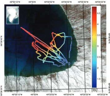
Fig. 2.Boat paths and measured depth values imposed over a high-resolution (0.5 m) Wordlview-2 image.
this choice is related to the strong absoprtion (e.g., low re-flectance) at wavelenghts above∼650 nm. As shown in the
literature (e.g., Sneed and Hamilton, 2007), this can be used to increase the sensitivity to lake detection with respect to the use of wavelengths around or below 650 nm. However, the strong absoprtion in the near-infrared region compromises the use of such band for depth retrieval. Because in this study we are mostly interested in assessing lake depth retrieval, rather than lake detection, we focus on wavelenghts below 650 nm. We also note that, as a consequence of the strong absorption by water in the near infrared region, in-situ spec-tral measurements in that band for lake depth above a few tens of centimeters were characterized by an extremely low signal/noise ratio (e.g., comparable to the dark current mea-surement) and were, therefore, excluded from our analysis. Measurements for lake depth values less than 1 m are also excluded from our analysis because of the relatively small sensitivity of the reflectance data in the Landsat and MODIS blue and green bands to shallow waters.
4 Analysis of in-situ data
The boat paths and the corresponding measured depth are superimposed in Fig. 2 on a high-resolution (0.5 m) image collected on 4 July 2010 by the WorldView-2 sensor (http://worldview2.digitalglobe.com/). Shallow waters are generally located along the edge of the lake, with depth increasing toward its center, up to ∼4.5 m. In Fig. 3 we
plot the in-situ water-leaving reflectance spectrally averaged over the Landsat band 1 (B1LANDSAT, 450–515 nm), band 2 (B2LANDSAT, 525–605 nm) and band 3 (B3LANDSAT, 630–690 nm) vs. the in-situ measured lake depth. In-situ
Fig. 3. In-situ measured water-leaving reflectance values vs. lake depth for the Landsat bands 1, 2 and 3 and exponential fitting.
measured water-leaving reflectance is fitted with Eq. (1), using Ad, g and R∞ as free fitting parameters. The
values obtained for g are: gB1 LANDSAT fit= 0.023 m−1, gB2 LANDSAT fit= 0.24 m−1 and gB3 LANDSAT fit= 0.81 m−1. The corresponding g values obtained assuming g= 2Kd (with Kd obtained from Pope and Fry, 1997) are gB1 LANDSAT 2Kd= 0.045 m−1, gB2 LANDSAT 2Kd= 0.21 m−1 and g
B3 LANDSAT 2Kd= 0.65 m−1. The fitted values of g are consistent with those computed assuming g= 2Kd, though differences exist.
To address these differences, we analyzed the spectral de-pendency of the bottom albedoAdand of the coefficientα. Figure 4a and b show, respectively, the values ofα(Fig. 4a) andAd(Fig. 4b) in the 450–650 nm region obtained by min-imizing the difference between measured water-leaving re-flectance values and those simulated using Eq. (1), withα, Ad and R∞ as free fitting parameters and z measured
in-situ. For convenience, the values forR∞are incorporated in
Fig. 4c, though this parameter is excluded from our analy-sis. The iterative fitting procedure terminates when the dif-ference between measured and simulated water leaving re-flectance,1R, is smaller than a threshold value1RT. The sensitivity of the fitting procedure to the choice of 1RT is shown Fig. 4, where bars represent the range of the fit-ted coefficients when1RT is set to 0.01, 0.025, 0.05 and 0.1. The spectrally averaged values for α for the Landsat bands 1 and 2 and the spectrally similar MODIS bands 3 and 4 are, respectively: αB1 LANDSAT=1.91, αB2 LANDSAT= 2.33,αB3 MODIS=1.73 andαB4 MODIS=2.4. For the lake under study, the optimal (fitted) values for α differ by ∼
+ 15 % (−15 %) from the constant value of α= 2. An er-ror of 15 % onαtranslates into a lake depth retrieval error of ∼17 % when using the Landsat band 2. Figure 4 also
Fig. 4.Spectral dependency ofα(top) andAd(bottom) values de-rived from the minimization of the difference1Rbetween mea-sured and theoretical water-leaving reflectance values. Bars repre-sent the range of values when different1Rvalues are used (see text for details).
easily explained, aside from a possible chlorophyll concen-tration in the water, currently considered to be unlikely. A possible explanation is a higher variability of lake-bottom albedo in the blue region, producing a higher degree of un-certainty in our approximatedαin that range.
The fitted values ofAdare greater at shorter wavelength and decrease with increasing wavelength, displaying a spec-tral behavior similar to that of glacier ice albedo (e.g., Gren-fell and Perovich, 2004). To evaluate the assumption of es-timating the value ofAdfrom the reflectance of shallow wa-ters, we use data collected by Landsat over Lake Olivia on 9 July 2010 (http://glovis.usgs.gov), converted into plane-tary reflectance following Chander et al. (2009). Though Landsat and in-situ data were not collected on the same day, we assume that the lake depth did not change con-siderably between 6 and 9 July. This is supported by the small depth change (<0.2 m) recorded by a pressure trans-ducer positioned into the lake during the period 1–6 July and by the simple visual analysis of daily WorldView-2 ra-diances collected between 4 and 9 July. Refletcance values at the top of the atmosphere (TOA) were corrected for at-mospheric effects using the Fast Line-of-sight Atat-mospheric Analysis of Spectral Hypercubes (FLAASH) atmospheric correction ( Alder-Golden et al., 1999) implemented in the software ENVI®. In absence of atmospheric data, to simu-late mid-summer conditions over the section of Greenland under study, the FLAASH model was initialized using a mid-latitude winter atmospheric model and maritime aerosol model. Aerosol optical depth was calculated using a 2-band VIS and SWIR ratio method using band 3 and 7 respectively
Fig. 5. Distribution of Advalues for the Landsat bands 1 and 2 estimated from Eq. (2) using lake depth measured by the boat (cont. lines) and of reflectance values from the edge lake (dashed lines).
( Kaufman et al., 1997). The average difference between at-mospherically corrected and TOA reflectance values over the lake was−3.9% (±0.98 %) in the case of band 1 and−2.4% (±2.1 %) for band 2. The choice of the atmospheric model
applied to the TOA reflectance values can be a source of un-certainty on the lake depth estimates. This unun-certainty cannot be estimated in absence of information on the vertical profile of the atmospheric parameters used in the model. However, we decided to use the atmospherically corrected reflectance values for our analysis for consistency with the MODIS data used in this study.
Figure 5 illustrates the distribution of Ad for the Land-sat band 1 (black lines) and band 2 (gray lines) ob-tained resolving Eq. (2) for Ad, with z obtained from in-situ measurements andR∞ from the Landsat image where
deep water (z>40 m) is present (e.g., Sneed and Hamil-ton, 2007). The distributions of the reflectance values at the two bands estimated from pixels along the lake edge are also plotted. The mean Ad values obtained from solving Eq. (2) are AdLANDSAT B1= 0.37±0.012 and AdLANDSAT B2= 0.3±0.024; the mean reflectance values for pixels along the lake edge are REdge B1= 0.42±0.058 for band 1 andREdge B2= 0.34±0.062 for band 2. The percent-age error between the meanAdvalue and the mean of the reflectance values along the lake edge is∼10 % in both cases
of the blue and green Landsat bands. From Eq. (2), this trans-lates into an average error on lake depth retrieval between
∼−10 % and∼−15 % when using, respectively, the Landsat
bands 1 or 2. The error on depth is maximum for shallow waters with an underestimation down to∼−25 % (blue) and
∼−40 % (green) and reduces to ∼−5 % for both channels for lake depth values up to 10 m.
5 Assessment of lake depth from satellite data
Table 2.Statistics on lake depth retrieval using different sensors, bands and hypothesis on the bottom albedo valuesAd.
Mean [m] Std. dev. [m] Max. [m] RMSE [m] MAE [m] Correlation % absolute error
SONAR
2.83 0.97 4.55 n/a n/a n/a n/a
Landsat
BAND 1 (450–515 nm)
Ad=µAdLANDSAT B1 2.98 1.62 5.68 0.99 0.65 0.78 3.71
Ad=µEdge B1 5.93 1.63 8.47 3.15 2.96 0.77 121.8
BAND 2 (525–605 nm)
Ad=µAdLANDSAT B2 3.01 0.98 4.57 0.63 0.51 0.85 4.21
Ad=µEdge B2 3.47 0.95 4.92 0.82 0.63 0.87 17.91
MODIS
BAND 3 (459–479 nm)
TERRA [2 through 5 July] 6.5 1.93 8.65 n/a n/a n/a n/a AQUA [2 through 5 July] 2.3 1.47 4.14 n/a n/a n/a n/a
BAND 4 (545–565 nm)
TERRA [2 through 5 July] 2.1 0.92 2.9 n/a n/a n/a n/a AQUA [2 through 5 July] 0.9 0.9 1.9 n/a n/a n/a n/a
of lake depth obtained from satellite data, together with the root mean square error, the mean absolute error, corre-lation and percentage error between spaceborne-estimated lake depth using either Landsat and 500 m MODIS re-flectance product (http://modis.gsfc.nasa.gov/data/dataprod/ dataproducts.php?MOD NUMBER=09) and the values mea-sured by the sonar. Results obtained from MODIS are av-eraged over the period 2–5 July 2010, when in situ data were collected. We decided to use the abovementioned MODIS product (rather than correcting level 1 MODIS data for atmopshere and extract reflectance values) because of the potential large use of such product in estimating spatio-temporal variability of supraglacial lakes at a relatively low computational cost. However, we point out that the MODIS reflectance product (MOD09) makes use of multi-ple daily observations. Within each tile, areas with clouds or low elevation sun angles are not used and other crite-ria are applied to select those observations used to gener-ate the product (http://modis-sr.ltdri.org/products/MOD09 UserGuide v1 3.pdf). Consequently data acquired at dif-ferent times can be potentially used for generating the final product. We also point out that the MODIS nominal spatial resolution of 250 m is only valid for those cases when the observation angle is close to nadir. When the target is on the side of the swath, the instantaneous field of view (IFOV) be-comes larger and, hence, a larger surface is responsible for the reflectance value. If this surface contains the lake edge, the overall reflectance might be higher than the one obtained
when the observation angle was close to nadir, because of the presence of ice or snow. Lastly, another factor affecting the remote sensing algorithm is the presence of ice on the lake surface, which has been observed from the analysis of high resolution visible images and during our fieldwork.
of 0.59 m. MODIS band 4 tends to underestimate lake depth with respect to in-situ data. In the case of MODIS, the use of theαfiitted value deteriorates the performance of the re-mote sensing algorithm, further reducing the values of the estimated lake depths.
In Table 2 we report the results of our analysis aimed at quantifying the error on lake depth retrieval from the assump-tions of a uniformAdvalue for the whole lake and using the reflectance values of the pixels at the edge of the lake forAd. Lake depth values are estimated using Eq. (2), withAdvalues given by the mean of the distributions of the bottom albedo values obtained form the concurrent analysis of surface and satellite data or by the mean of the reflectance values along the lake edge. The table includes the mean, standard devia-tion, maximum value of lake depth obtained from the satellite data together with the root mean square error, the mean abso-lute error, correlation and percentage error between the lake depth values estimated with the different configurations and the values measured by the sonar. Results from both Landsat (bands 1 and 2) and MODIS (bands 3 and 4) are reported. In general, best results are obtained when using the Landsat band 2 whenAdis given by the mean of theAddistribution computed from the conjunct analysis of satellite and surface data. Depth estimates using Landsat band 1 show a larger standard deviation and higher maximum depth values (above the maximum measured depth), likely as a consequence of the smaller diffuse attenuation coefficient in the blue band (Smith and Baker, 1980; Pope and Fry, 1997). Maximum lake depth values estimated when using Landsat band 2 are closer to the value measured in situ. The MODIS sensor on TERRA provides smaller lake depth values than those ob-tained with the one mounted on AQUA. Given the short time-series it is not possible to assess whether this is a consistent bias. The values estimated by MODIS on TERRA are the closest to those estimated by Landsat and measured in situ. Lake depth values estimated from MODIS when using band 4 are generally smaller than those measured in situ.
6 Conclusions and future work
We collected in-situ concurrent multi-spectral and depth ob-servations over a supraglacial lake in West Greenland in or-der to assess spaceborne bathymetry. Such measurements allowed us to study the spectral dependency of the bottom albedoAdand coefficientαwith the latter linearly relating the attenuation coefficientgand the diffuse attenuation fac-torKd. Results show that, as expected, the spectral behavior ofAdis similar to that of glacier ice albedo. The increase ofα with wavelength from in-situ data cannot be easily explained without assuming chlorophyll, or other absorbing material, in the water, which is present in very minimal concentrations according to our preliminary analysis of water samples. One explanation for the spectral behavior ofαis that the bottom albedo has a higher variability in the blue region, attributing
some of the loss due to a darker blue ice to loss along the water column.
We assessed a widely used literature technique in which Adis assumed to be uniform and equal to the reflectance of shallow waters along the lake edge. The analysis of in-situ measurements show a Gaussian-like behavior ofAd,with this variability appearing to be intrinsic to the albedo of the bot-tom, consisting of large patches of cryoconite. The differ-ence between the meanAdvalue obtained from in-situ mea-surements and the mean of the reflectance values along the lake edge obtained from Landsat is on the order of∼10 %.
This translates into an average error on lake depth retrieval of
−11.8 % (−15.9 %) when using the Landsat band 1 (band 2).
The error is maximum for shallow waters with an underesti-mation down to−23.7 % (−42.7%) and reduces to−4.6 % (−4.7 %) for lake depth values up to 10 m.
In the case ofα, the values obtained from in-situ measure-ments differ by∼15 % from those computed using literature approaches. Best spaceborne-based estimates were obtained when using either the Landsat band 2 or the spectrally sim-ilar MODIS band 4. In the case of Landsat, best results are obtained when using theαvalue derived from in-situ mea-surements (α= 2.33. However, this is not true in the case of MODIS, where best results are obtained using the values suggested in the literature (α= 2). In the case of MODIS, however, mixed-pixel effects and relatively coarse resolution can be responsible for large uncertainty. For example, the presence of ice within a pixel will increase the reflectance with respect to a pixel containing only liquid water, leading to an underestimation of the lake depth. This is especially true for relatively small lakes and for those pixels contain-ing the lake edges. In the future, we plan to collect a more comprehensive in-situ data set on the inherent optical proper-ties of melt pond water and to extend our analysis to multiple lakes. We also plan to use a more sophisticated model of the water column (Lee, 1999), in which depth estimations can be made with a fully physical model of water constituents.
Acknowledgements. This work was supported by the NSF grant ANS 0909388 and by the NASA Cryosphere Program. Fieldwork activities were partially supported by the World Wildlife Foun-dation (WWF). Thanks to Mark Jenkins (National Geographic), James Balog and Adam Lewinter (Extreme Ice Survey, EIS) for sharing their fieldwork knowledge and their logistical support. We are deeply grateful to Jim “Soup” Rios for leading the safety and rescue section of our camp and for logistical support at Lake Olivia. Thanks to Gordon Hamilton and an anonymous reviewer for their suggestions aimed at improving the quality of this manuscript. We also thank Tristan Schwartzman for processing the boat data at CCNY.
References
Adler-Golden, S. M., Matthew, M. W., Bernstein, L. S., Levine, R. Y., Berk, A., Richtsmeier, S. C., Acharya, P. K., Anderson, G. P., Felde, G., Gardner, J., Hoke, M., Jeong, L. S., Pukall, B., Ratkowski, A., and Burke H.-H.: Atmospheric Correction for Short-wave Spectral Imagery Based on MODTRAN4. SPIE Proc. Imaging Spectrom., 3753, 61–69, 1999.
Box, J. E. and Ski, K.: Remote sounding of Greenland supra-glacial melt lakes: implications to sub-glacial hydraulics, J. Glaciol., 181, 257–265, 2007.
Chander, G., Markham, B. L., and Helder, D. L.: Summary of cur-rent radiometric calibration coefficients for Landsat MSS, TM, ETM+, and EO-1 ALI sensors, Remote Sens. Environ., 113, 893–903, 2009.
Das, S. B., I. Joughin, M. D. Behn, I. M. Howat, M. A. King, D. Lizarralde and M. P. Bhatia: Fracture propagation to the base of the Greenland ice sheet during supraglacial lake drainage, Sci-ence, 320, 778–781, 2008.
Georgiu, S., Shepherd, A., McMillan, M., and Nienow, P.: Sea-sonal evolution of supraglacial lake volume from ASTER im-agery, Ann. Glaciol., 50(52), 95–100, 2009.
Grenfell, T. C. and Perovich, D. K.: Seasonal and spatial evolu-tion of albedo in a snow-ice-land-ocean environment, J. Geo-phys. Res., 109, C01001, doi:10.1029/2003JC001866, 2004. Joughin, I., Tulaczyk, S., Fahnestock, M., and Kwok, R.: A
mini-surge on the Ryder Glacier, Greenland, observed by satellite radar interferometry, Science, 274, 228–230, 1996.
Kaufmann, Y. J., Wald, A. E., Remer, L. A., Gao, B.-C., Li, R.-R., and Flynn, L.: The MODIS 2.1-mm Channel-Correlation with Visible Reflectance for Use in Remote Sensing of Aerosol. IEEE T. Geosci. Remote Sens., 35, 1286–1298, 1997.
Lee, Z., Carder, K. L., Mobley, C. D., Steward, R. G., and Patch, J. S.: Hyperspectral remote sensing for shallow waters. 2. Deriv-ing bottom depths and water properties by optimization, Appl. Optics, 38(18), 3831–3843, 1999.
L¨uthje, M., Pedersen, L. T., Reeh, N., and Greuell, W.: Modelling the evolution of supra-glacial lakes on the West Greenland ice-sheet margin, J. Glaciol., 52, 608–618, 2006.
Maritorena, S., Morel, A., and Gentili, B.: Diffuse reflectance of oceanic shallow waters: Influence of water depth and bottom albedo, Limnol. Oceanogr., 39(7), 1689–1703, 1994
McMillan, M., Nienow, P., Shepherd, A., Benham, T., and Sole, A.: Seasonal evolution of supra-glacial lakes on the Greenland ice sheet, Earth Planet. Sci. Lett., 262, 484–492, 2007.
Mobley, C. D.: Estimation of the remote-sensing reflectance from above-surface measurements, Appl. Optics, 38(36), 7442-7455, 1997.
Mueller, J.: In-Water Radiometric Profile Measurements and Data Analysis Protocols, NASA/TM-2003-21621/Rev-Vol III, 7, 2003.
Mueller, J., McClain, G., Bidigare, R., Trees, C., Balch, W., Dore, J., Drapeau, D., Karl, D., and Van, L.: Ocean optics protocols for satellite ocean color sensor validation, revision 5, volume V: Biogeochemical and bio-optical measurements and data analysis protocols, NASA Tech. Memo. 2003-211621, Rev, 5, 2003. Philpot, W. D.: Bathymetric mapping with passive multispectral
imagery, Appl. Optics, 28(8), 1569–1578, 1989.
Pimentel, S. and Flowers, G. E.: A numerical study of hydrologi-cally driven glacier dynamics and subglacial flooding, Proc. R. Soc. A, 467, 537–558, doi:10.1098/rspa.2010.0211, 2011. Pope, R. M. and Fry, E. S.: Absorption spectrum (380–700 nm) of
pure water. II. Integrating cavity measurements, Appl. Opt., 36, 8710–8723, 1997.
Smith, R. C. and Baker, K. S.: Optical properties of the clear-est natural waters (200–800 nm), Appl. Optics, 20(2), 177–184, doi:10.1364/AO.20.000177, 1981.
Sneed, W. A. and Hamilton, G. S.: Evolution of melt pond volume on the surface of the Greenland Ice Sheet, Geophys. Res. Lett., 34, L03501, doi:10.1029/2006GL028697, 2007.
Sundal, A. V., Shepherd, A., Nienow, P., Hanna, E., Palmer, S., and Huybrechts, P.: Evolution of supra-glacial lakes across the Greenland Ice Sheet, Remote Sens. Environ., 113, 2164–2171, 2009.