www.atmos-chem-phys.net/15/6577/2015/ doi:10.5194/acp-15-6577-2015
© Author(s) 2015. CC Attribution 3.0 License.
Momentum forcing of the quasi-biennial oscillation by equatorial
waves in recent reanalyses
Y.-H. Kim and H.-Y. Chun
Department of Atmospheric Sciences, Yonsei University, Seoul, South Korea Correspondence to:H.-Y. Chun ([email protected])
Received: 12 January 2015 – Published in Atmos. Chem. Phys. Discuss.: 24 February 2015 Revised: 20 May 2015 – Accepted: 31 May 2015 – Published: 16 June 2015
Abstract. The momentum forcing of the QBO (quasi-biennial oscillation) by equatorial waves is estimated us-ing recent reanalyses. Based on the estimation usus-ing the conventional pressure-level data sets, the forcing by the Kelvin waves (3–9 m s−1month−1) dominates the net forcing by all equatorial wave modes (3–11 m s−1month−1) in the easterly-to-westerly transition phase at 30 hPa. In the oppo-site phase, the net forcing by equatorial wave modes is small (1–5 m s−1month−1). By comparing the results with those from the native model-level data set of the ERA-Interim re-analysis, it is suggested that the use of conventional-level data causes the Kelvin wave forcing to be underestimated by 2–4 m s−1month−1. The momentum forcing by mesoscale gravity waves, which are unresolved in the reanalyses, is de-duced from the residual of the zonal wind tendency equa-tion. In the easterly-to-westerly transition phase at 30 hPa, the mesoscale gravity wave forcing is found to be smaller than the resolved wave forcing, whereas the gravity wave forcing dominates over the resolved wave forcing in the op-posite phase. Finally, we discuss the uncertainties in the wave forcing estimates using the reanalyses.
1 Introduction
The quasi-biennial oscillation (QBO) is the predominant variability of the tropical stratosphere with periods of about 20–35 months (Baldwin et al., 2001). The QBO is most prominent in the zonal wind field, alternating between east-erly and westeast-erly. The alternating jets modulate interannual extratropical wave activities and impact on the strength of the polar stratospheric vortex (Holton and Tan, 1980; Wat-son and Gray, 2014). The QBO also induces the secondary
meridional circulation (Plumb and Bell, 1982), which mod-ulates the distribution of chemical species in the tropics and extratropics (Hilsenrath and Schlesinger, 1981; Li and Tung, 2014). For these reasons, it is important to understand and model the QBO. In practice, such modulations of the polar vortex and chemical species distributions cannot be repro-duced by global models in which the QBO is not simulated.
CAM5 (Richter et al., 2014) models, the PGW forcing is dominant in both phases at this altitude. Therefore, it is nec-essary to quantitatively constrain the forcing due to equato-rial waves based on observations, which motivates this study. It is difficult to directly measure the momentum forc-ing due to equatorial waves from observations, as this re-quires the simultaneous measurement of horizontal and ver-tical winds. Instead, for the Kelvin and gravity waves, mo-mentum forcing has been estimated from temperature mea-surements (and sometimes along with the zonal wind) given by radiosonde and satellites using gravity wave theory (e.g., Sato et al., 1997; Ern and Preusse, 2009; Alexander and Or-tland, 2010; Ern et al., 2014). An alternative to estimations from measurements is to use reanalyses. In the equatorial lower stratosphere, the horizontal wind and temperature data from radiosonde observations are assimilated in the reanaly-ses, along with satellite-observed temperature data from after 1979. It should be noted, however, that the vertical veloc-ity is poorly constrained in the reanalyses. This might result in a spread of estimated wave forcings between the reanal-yses, along with many other factors (e.g., different assimila-tion processes).
This study aims to estimate the momentum forcing due to equatorial waves in the reanalysis data sets. The equa-torial waves resolved in the reanalyses are classified into Kelvin, mixed Rossby-gravity, inertio-gravity, and Rossby waves, and the forcing from each wave type is estimated. In addition, the forcing by smaller-scale waves that are un-resolved in the reanalyses is also estimated by comparing the resolved wave forcing with the total forcing required for the QBO progression.
2 Data and method
Four recent reanalyses are used: the ECMWF (European Centre for Medium-Range Weather Forecasts) Interim Re-analysis (ERA-I; Dee et al., 2011), Modern-Era Retrospec-tive Analysis for Research and Applications (MERRA; Rie-necker et al., 2011), Climate Forecast System Reanalysis (CFSR; Saha et al., 2010), and Japanese 55-year Reanalysis (JRA-55; Kobayashi et al., 2015). The resolutions of these reanalyses are presented in Table 1. The horizontal resolu-tions of the native models for these reanalyses range from 0.38 to 0.7◦. The models have 10–13 vertical levels between about 70 and 10 hPa. The reanalysis data sets are available for variables that are interpolated vertically to the conven-tional pressure (p) levels (e.g., 100, 70, 50, 30, 20, 10, and 7 hPa) from the model levels. In this study, we use p-level data sets with horizontal resolutions reduced to around 21h, where1his the native resolution of the model (see Table 1). Provided that the effective resolution of weather prediction models is typically coarser than 41h(e.g., Skamarock et al., 2014), a horizontal resolution of∼21his sufficient to an-alyze the equatorial waves resolved by these reanalyses. To
Table 1.Horizontal resolution of the native models and pressure-level data sets for the four reanalyses used in this study, along with the number of vertical levels at 70–10 hPa.
Model resolution Data resolution used (number of levels at 70–10 hPa) ERA-I TL255∼0.7◦(10) 1.5◦(5) MERRA 0.5◦×0.667◦(12) 1.25◦(6) CFSR T382∼0.38◦(13) 1.0◦(5)
JRA-55 TL319∼0.56◦(10) 1.25◦(5)
examine the sensitivity of the wave forcing estimation to the vertical level of the reanalysis data sets, we also use the na-tive model-level data set of ERA-I. The temporal resolution of the data used is 3 h for MERRA and 6 h for the others. Additionally, we calculated the wave forcing estimates using 6-hourly subsampled MERRA data (not shown), and con-firmed that the difference between the results from 3- and 6-hourly data is negligible. The data in all reanalyses cover the period 1979–2010.
The zonal momentum forcing due to stratospheric waves is calculated in the transformed Eulerian-mean (TEM) equation (Andrews et al., 1987):
ut=v∗hf−(acosφ)−1(ucosφ)φi−w∗uz
+(ρ0acosφ)−1∇ ·F+X. (1)
The notation follows the conventions described in Andrews et al. (1987). Here, F= F(φ), F(z)
is the Eliassen–Palm (E–P) flux, defined by
F(φ)=ρ0acosφuzv′θ′/θz−v′u′
, (2)
F(z)=ρ0acosφnhf−(acosφ)−1(ucosφ)φ i
v′θ′/θ z−w′u′
o
. (3)
alsoX. Equation (1), the TEM equation for pressure coordi-nates, is used for the model-level data set as well as for the
p-level data sets, as the model level of ERA-I above 73 hPa (∼18 km) is on the constant pressure level.
The momentum forcing produced by each of the equa-torial modes can be calculated after separating the pertur-bations in Eqs. (2) and (3) into each wave mode, follow-ing Kim and Chun (2015, KC15 hereafter). The separation of wave modes is explained in detail in Sect. 4 of KC15, and is briefly described here. The perturbation variables are split into symmetric and anti-symmetric components with respect to the Equator, and each component is transformed to the zonal wavenumber–frequency (k–ω) domain. In the symmetric spectrum, the perturbations for the Kelvin waves are restricted to 0< k≤20 and ω <0.75 cycle day−1, and those for the mixed Rossby-gravity (MRG) waves are re-stricted to |k| ≤20 and 0.1≤ω≤0.5 cycle day−1 in the anti-symmetric spectrum. In this paper, the MRG waves refer to both the westward and eastward propagatingn=0 waves. The two equatorial modes are further restricted in the spectral components (k,ω) by requiring|F(z,H )|<|F(z,M)|(Kelvin waves) and F(z,H )F(z,M)<0 (MRG waves) (see KC15), whereF(z,H )andF(z,M)are the contributions of the merid-ional heat flux and vertical momentum flux toF(z)(i.e., the first and second terms on the right-hand side of Eq. 3), re-spectively, for a given (k,ω). Spectral components that are not defined as Kelvin or MRG waves are classified as Rossby waves if |k| ≤20 and ω≤0.4 cycle day−1, and as inertio-gravity (IG) waves otherwise. After separating the perturba-tions into the four wave modes, the forcing is calculated by
(ρ0acosφ)−1∇ ·FW, whereFWrepresents the E–P flux due to each mode.
3 Results
3.1 Momentum forcing by the waves resolved in the reanalyses
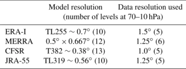
The time–height cross sections of the forcing by equatorial waves, averaged over 5◦N–5◦S regions, are shown in Fig. 1, where model-level data from ERA-I have been used for re-cent years (2003–2010). For all figures in this paper except Fig. 5, the ticks on the horizontal axis correspond to 1 Jan-uary of the given years. The eastward forcing by the Kelvin waves appears in the QBO phase of strong westerly shear. The MRG waves induce westward forcing in both phases of the westerly and easterly shear, with comparable magnitudes between the phases (Kawatani et al., 2010a, b, and KC15). The MRG wave forcing is primarily by the westward prop-agating mode not only in the easterly shear but also in the westerly shear (not shown), which may suggest the possibil-ity of stratospheric generation of the wave above the easterly jet (see Maury and Lott, 2014, and KC15). For the Kelvin and MRG waves, the altitude and magnitude of the maximum
Figure 1.Time–height cross sections of the zonal momentum forc-ing by the Kelvin, MRG, IG, and Rossby waves (from top to bot-tom) averaged over 5◦N–5◦S, obtained using the model-level data
of ERA-I over the period 2003–2010 (shading). The MRG wave forcing is multiplied by 3. The zonal mean wind over 5◦N–5◦S
is superimposed at intervals of 10 m s−1(contour). The thin solid, dashed, and thick solid lines indicate westerly, easterly, and zero wind, respectively.
forcing in each QBO cycle vary significantly. The IG waves provide eastward and westward forcing in the westerly and easterly shear phases, respectively. The Rossby wave forcing is strong in the upper stratosphere. Unlike the other waves, the Rossby wave forcing is not aligned with the strong-shear phases of the QBO at altitudes below 30 km. Rather, it has significant magnitudes in the northern winters and summers and is weakened in the following seasons. In addition, this forcing does not appear in the strong easterlies of the QBO, as the Rossby waves do not propagate easily with the easterly background wind. These features in the vertical structure of the equatorial wave forcing are generally similar between the reanalysis data sets (not shown). Here, we select three levels, 50, 30, and 10 hPa, to assess the wave forcing in the reanaly-ses in detail. Note that the level of 10 hPa is close to the upper limit of the sonde sounding assimilated to the reanalyses.
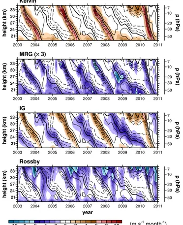
Figure 2.Zonal momentum forcing by the Kelvin, MRG, IG, and Rossby waves averaged over 5◦N–5◦S at 30 hPa for the period 1979–2010, as well as the net forcing by all resolved waves (from top to bottom) obtained using thep-level data of ERA-I (blue), MERRA (red), CFSR (green), and JRA-55 (orange). The phase of the maximum easterly and westerly in each QBO cycle at 30 hPa is indicated by the dashed and solid vertical lines, respectively. The difference between upper and lower bounds of the wave forcing calculated from each data set is also indicated (gray shading).
as the net forcing due to all resolved waves. The spread be-tween the four reanalyses (i.e., the difference bebe-tween up-per and lower bounds of the wave forcing estimated from each data set) is also indicated (gray shading). The phases of the maximum easterly (westerly) in each QBO cycle at 30 hPa are indicated by the dashed (solid) vertical lines in Fig. 2. The temporal evolution of the equatorial wave forc-ing is, at the first order, consistent between the data sets. The peak magnitude of the Kelvin wave forcing in the E– W phase shows similar cycle-to-cycle variations in all re-analyses. For instance, the Kelvin wave forcing in the four reanalyses is strong in 2010 (7.1–8.7 m s−1month−1) and weak in 1992 (2.8–4.7 m s−1month−1; here, the month in the unit of forcing refers to 30 days regardless of the month). Prior to around 1993, the MRG wave forcing in the re-analyses seems relatively sporadic and weak compared to afterward, although the forcing in 1980 and 1985 has ex-ceptionally large peaks in MERRA. The magnitude of the MRG wave forcing reaches∼2 m s−1month−1. The IG wave forcing varies between −3 and 4 m s−1month−1,
follow-ing the QBO phase. The Rossby wave forcfollow-ing magnitude is less than or similar to∼2 m s−1month−1 in most years, except in 1980, 1988, and 2008 for CFSR and ERA-I (3– 3.5 m s−1month−1). The net wave forcing has large posi-tive peaks in the E–W phases (3.4–11 m s−1month−1), due mainly to the Kelvin waves, and is negative during the W– E phases (1.5–5.2 m s−1month−1) by the IG, MRG, and Rossby waves (Fig. 2). The peak forcing ranges during the E–W and W–E phases are summarized for each wave in Ta-ble 2.
Figure 3.The same as in Fig. 2, except using the model-level data (black) along with thep-level data (blue) for ERA-I.
to about 4 m s−1month−1. There are many potential causes for this spread of forcing magnitudes between the reanaly-ses. For instance, each reanalysis used a different assimila-tion method, assimilated different observaassimila-tional data, and es-sentially used a different forecast model (e.g., in terms of model dynamics and resolutions). In addition, the species and numbers of assimilated observational data for a single re-analysis are dependent on time, particularly the satellite data. This makes the further investigation of temporal variations in wave forcing complicated. Therefore, in this study, we focus on assessing the range of wave forcing revealed by the re-analyses and do not speculate on the causes of the spread, or temporal variations, in the reanalyses.
Figure 3 shows the wave forcing at 30 hPa calculated us-ing the model-level data of ERA-I (ERA-I_ml) along with that using thep-level data of ERA-I. The plot exhibits robust differences in Kelvin and IG wave forcing between the two data sets. The peaks of the Kelvin wave forcing in the E–W phase from ERA-I_ml range from 6.7 to 13 m s−1month−1, which are 2–4 m s−1month−1 larger than those from ERA-I. The IG wave forcing from ERA-I_ml has positive and negative peaks that are 0.8–2.7 m s−1month−1 larger than those from ERA-I. The differences in the MRG and Rossby wave forcing depend on the year and are typically less than
∼1 m s−1month−1. The net wave forcing in the E–W (W–
E) phase is 4–9 m s−1month−1 (1–4 m s−1month−1) larger in the model-level result than in thep-level output.
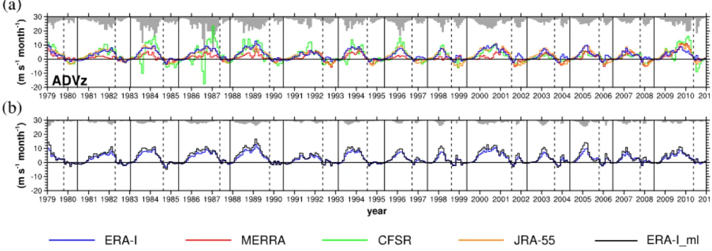
Figure 4.The same as in(a)Fig. 2 and(b)Fig. 3, except for the vertical advection of zonal wind.
Table 2. Phase-maximum magnitudes of the Kelvin, MRG, IG, and Rossby wave forcing, net-resolved wave forcing,X, andX∗
[m s−1month−1] at 30 hPa in the E–W and W–E phases for the pe-riod 1979–2010, obtained using thep-level data sets and the ERA-I model-level data set. Details ofXandX∗can be found from the text along with Eqs. (1) and (4). Positive forcing is denoted by bold font.
E–W W–E
p-level model-level p-level model-level
Kelvin 2.8–8.7 6.7–13
MRG 0.6–2.1 0.6–1.8 0.2–1.8 0.6–2.6 IG 0.9–3.9 2.5–4.3 0.6–3.0 1.9–5.4 Rossby 0.7–2.7 0.6–2.9 0.7–3.5 0.9–3.8 Net-resolved 3.4–11 8.0–19 1.5–5.2 3.3–7.5 X 5.8–17 3.1–11 6.6–21 11–18
X∗ 5.8–14 11–21
This results in substantial differences between the two data sets, as shown in Fig. 3. The same may also be true for the other reanalyses. Unfortunately, not all the reanalyses pro-vide model-level data sets. However, the vertical resolution of the native models in the lower stratosphere is comparable across all reanalyses (Table 1). Thus, the magnitude of the wave forcing obtained from the p-level data sets of reanal-yses other than ERA-I (Fig. 2) should also be considered as underestimated, potentially by amounts comparable to those in ERA-I.
3.2 Estimated momentum forcing by the waves unresolved in the reanalyses
As mentioned in Sect. 2, the term X in Eq. (1) represents the zonal forcing by unresolved mesoscale gravity waves and turbulent diffusion, and is also influenced by the resolved-scale processes that are erroneously represented in the re-analyses. If one assumes that the resolved-scale processes are well represented in the reanalyses, the forcing by
unre-solved processes can be approximated asX. In this section, we calculate the vertical advection of zonal wind (the second term on the right-hand side of Eq. (1), ADVz hereafter) and estimate the range ofXin the reanalyses. A discussion of the above assumption is included in the next section.
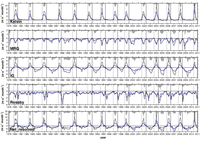
Figure 4a shows ADVz, obtained using the p-level data of the four reanalyses. The peak magnitude of ADVz in the W–E phase is around 10 m s−1month−1, and that in the E–W phase is typically 1–4 m s−1month−1 (excluding the anomalously large peaks in 1983 and 1986–1987 in CFSR). Note that ADVz in the W–E phase is much larger than the net-resolved wave forcing in the same phase (1.5– 5.2 m s−1month−1; Table 2), and the two terms have oppo-site signs. There exist some robust ADVz features in the W– E phase: ADVz is very similar in ERA-I and JRA-55, and ADVz in MERRA is about half of that in ERA-I or JRA-55 in many years. As a result, the spread between the reanalyses is quite large (∼10 m s−1month−1) in this phase (Fig. 4a).
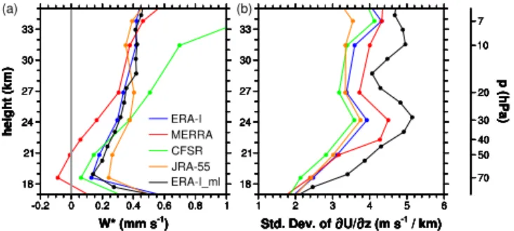
The large spread in the W–E phase between the different reanalyses suggests that the ADVz values obtained from the reanalyses are highly uncertain. Moreover, it is speculated that this spread may result in a large spread inX, as will be seen later. Therefore, the difference in ADVz between the reanalyses is further investigated by comparingw∗ and the vertical shear of zonal wind (uz). Figure 5a shows the clima-tologies ofw∗obtained from each data set. The profiles ofw∗
(a) (b)
Figure 5. (a)Mean residual vertical velocity and(b)standard devia-tion of the monthly and zonal mean wind shear for the period 1979– 2010 averaged over 5◦N–5◦S, obtained using thep-level data of ERA-I (blue), MERRA (red), CFSR (green), and JRA-55 (orange) as well as the model-level data of ERA-I (black).
causes ADVz to be underestimated (see Fig. 4a) and con-tributes to the large spread of ADVz.
Figure 5b shows the standard deviation of uz obtained from each reanalysis data set. These values are governed by the magnitude ofuzthat alternates between positive and negative with the QBO phase. Note that the difference in monthly and zonal mean wind between the reanalyses is small (not shown). Therefore,uzis mainly dependent on the intervals between theplevels. The standard deviation ofuz in ERA-I, CFSR, and JRA-55 is similar, as they have the sameplevels. MERRA has one moreplevel, at 40 hPa, and thus the magnitude of uz near 40 hPa in MERRA is larger than in the others. In all of the reanalyses, the limited sam-pling across vertical levels causes the magnitude of uz ob-tained from thep-level data sets to be underestimated com-pared touzfrom the model-level data (Fig. 5b). This implies that, as for the wave forcing, the ADVz values from thep -level data sets should also be considered as underestimations. The ADVz obtained from ERA-I_ml is presented in Fig. 4b. It can be seen that ADVz in the W–E phase from ERA-I_ml is consistently 2–4 m s−1month−1greater than that from the p-level data. Although this magnitude of difference between the p- and model-level data seems small in Fig. 4b, it can have a significant effect in the estimation ofXwhich has typ-ical values of∼10 m s−1month−1as will be shown later. The Coriolis force and meridional advection terms in Eq. (1) are generally small near the equatorial lower stratosphere (not shown).
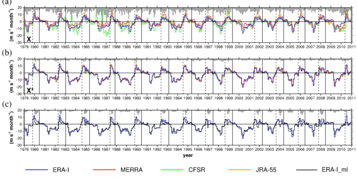
Figure 6a shows the value of X at 30 hPa obtained from thep-level data sets of the reanalyses. The positive peaks of
X in the E–W phase range from 5.8 to 17 m s−1month−1, and the negative peaks in the W–E phases vary from 6.6 to 21 m s−1month−1.Xin the E–W phase is about 50 % larger than the net resolved wave forcing (3.4–11 m s−1month−1), and that in the W–E phase is much larger than the net re-solved wave forcing (1.5–5.2 m s−1month−1). The spread in Xbetween the reanalyses is up to 10 m s−1month−1, except in 1983 and 1986–1987, when the ADVz in CFSR has
ab-normally large peaks (Fig. 4a). The large spread inXcould be expected because of the large spread in ADVz (Fig. 4a). From Fig. 5a, we can see that a large portion of the spread in ADVz is due to the underestimated vertical velocity in MERRA. Additionally, the zonal wind shear is underesti-mated in all of thep-level data sets. Therefore, we attempt to partly correct the estimates ofXvia an additional calcu-lation (X∗). In this calculation, ERA-I_ml is considered as reference data for all the terms in Eq. (1), except for the wave forcing term.X∗is estimated as
X∗=
n
ut−v∗hf−(acosφ)−1(ucosφ)φi+w∗uz or
−(ρ0acosφ)−1∇ ·F, (4)
where a superscript r denotes terms calculated using the ref-erence data, and the E–P flux divergence term is calculated using the respective reanalyses. X∗ is plotted in Fig. 6b. The negative peaks ofX∗in the W–E phase are larger than those ofXby 5–12 m s−1month−1, particularly for MERRA. The changes in positive peaks do not appear to be large. The spread in X∗ is up to ∼4 m s−1month−1, which re-sults from the spread in resolved wave forcing (see Eq. 4). Finally, X∗ in ERA-I_ml is shown in Fig. 6c. The posi-tive peaks of X∗ in the E–W phase in ERA-I_ml are 3.1– 11 m s−1month−1, and the negative peaks in the W–E phase are 11–18 m s−1month−1. These values ofX∗are compara-ble with those estimated by Ern et al. (2014). The positive peaks are smaller than those of the Kelvin wave forcing, suggesting that the peak magnitudes of the net mesoscale gravity wave forcing in the E–W phase at 30 hPa might be smaller than those of the Kelvin wave forcing. In contrast, the large negative values ofX∗ suggest that gravity waves are the dominant contributors to QBO in the W–E phase, as-suming that the turbulent diffusion is not of comparable mag-nitude. These results are consistent with those from previous studies using mechanistic, general circulation, or mesoscale models (e.g., Dunkerton, 1997; Giorgetta et al., 2006; Evan et al., 2012).
The wave forcing estimates at 50 and 10 hPa are also pre-sented in Tables 3 and 4, respectively. From Tables 2–4, it is shown that the Kelvin wave forcing in the E–W phase tends to increase with height from 2.7–9.2 m s−1month−1at 50 hPa to 2.2–15 m s−1month−1at 10 hPa, and the IG wave forcing from 0.5–2.5 to 0.5–6.2 m s−1month−1. The Rossby wave forcing exhibits an abrupt change between 30 and 10 hPa, and it reaches 14 m s−1month−1at 10 hPa in the W–E phase (see also Fig. 1).X∗depends significantly on the height, so that it is twice as large at 10 hPa as at 50 hPa in both phases. This may reflect an increase in mesoscale gravity wave forc-ing at 10 hPa in both phases of the QBO. However, it should be noted that the spread in resolved wave forcing, ADVz, and
Figure 6.The same as in Fig. 2, except for the terms(a)X,(b)X∗, and(c)as in Fig. 3 forX∗(see the text for a definition of these terms).
Table 3.The same as in Table 2, except at 50 hPa.
E–W W–E
p-level model-level p-level model-level
Kelvin 2.7–6.8 4.6–9.2
MRG 0.6–1.6 0.6–1.7 0.6–2.3 0.8–2.2 IG 0.5–2.3 1.3–2.5 0.4–2.4 1.4–3.7 Rossby 1.1–5.0 1.3–3.6 0.7–4.0 1.2–3.1 Net-resolved 2.8–8.8 5.4–11 0.9–6.4 2.7–6.2 X 3.7–10 2.2–4.3 0.5–17 6.9–13 X∗ 3.5–8.7 7.7–16
near 10 hPa in the reanalyses, owing to the vertical coverage of radiosonde observations. We additionally calculated the wave forcing estimates averaged over 10◦N–10◦S at 30 hPa (Figs. S1–S3 in the Supplement). The results are generally similar with those for 5◦N–5◦S (Figs. 2, 3, 6), except that the Kelvin (MRG) wave forcing is about 31 % (10–70 %) smaller when averaged over 10◦N–10◦S.
4 Summary and discussions
We have examined four reanalyses with the aim of esti-mating the momentum forcing of the QBO due to equato-rial waves over the period 1979–2010. The temporal evolu-tion of the forcing by equatorial wave modes is generally consistent between the reanalyses. The range of forcing by each wave mode is summarized in Tables 2–4. In the esti-mates for the E–W phase using the p-level data sets from the four reanalyses, the Kelvin wave forcing at 30 hPa (2.8– 8.7 m s−1month−1) was found to dominate the net wave
forc-Table 4.The same as in Table 2, except at 10 hPa.
E–W W–E
p-level model-level p-level model-level
Kelvin 2.2–12 3.6–15
MRG 0.4–5.3 0.2–3.6 0.4–2.3 0.5–1.8 IG 0.5–4.9 2.7–6.2 0.6–4.5 2.7–5.9 Rossby 0.7–8.0 2.2–8.4 4.3–12 6.1–14 Net-resolved 2.8–17 4.1–21 6.2–15 8.0–17 X 5.5–31 4.7–16 3.1–35 5.9–25 X∗ 4.1–17 6.3–30
ing resolved in the data sets (3.4–11 m s−1month−1). The forcing due to the MRG, IG, and Rossby waves in the W– E phase was found to be small, with a net forcing of 1.5– 5.2 m s−1month−1. The momentum forcing by processes that are not resolved in the reanalyses, which may be dominated by the mesoscale gravity waves, was also estimated. The unresolved forcing in the E–W phase ranges from 5.8 to 14 m s−1month−1 and that in the W–E phase from 11 to 21 m s−1month−1.
There exist uncertainties in the resolved-scale waves in the reanalyses even for the model-level data. As discussed in Sect. 3.1, the substantial difference between the wave forcing from the model-level data and from the interpolatedp-level data implies that a significant amount of waves with vertical wavelengths of about 2.8–5.6 km are present in the model-level data. Given that these vertical wavelengths are at the lower bound of the ranges captured by the forecast models (21v–41v), we can speculate that a substantial fraction of short-wavelength waves could remain under-represented in the reanalyses at the native model levels. The MRG and IG waves have vertical wavelengths that may be affected by this phenomenon. In a previous study by Ern et al. (2008), it was shown that the amplitudes of the MRG and IG waves in the ECMWF analysis are smaller than those from the SABER (Sounding of the Atmosphere using Broadband Emission Radiometry) observations. A number of studies using gen-eral circulation models (Boville and Randel, 1992; Giorgetta et al., 2006; Choi and Chun, 2008; Richter et al., 2014) have also demonstrated the need for high vertical resolutions (500–700 km) to capture equatorial waves; these are twice the resolution of the reanalyses used in this study.
There is another important source of uncertainty. The un-resolved gravity wave forcing has been deduced from the other forcing terms in the zonal wind tendency equation. In the W–E phase, the estimate of the unresolved forcing is highly dependent on the vertical advection term. However, as seen in Fig. 5a, the vertical velocity is poorly constrained in the reanalyses, and this introduces a large uncertainty in the vertical advection term. The spread in vertical advection be-tween the reanalyses reaches∼10 m s−1month−1. The val-idation of the vertical velocity field in the equatorial lower stratosphere in the reanalyses might be crucial for deduc-ing the unresolved-scale wave contribution to the QBO (Ern et al., 2014).
The Supplement related to this article is available online at doi:10.5194/acp-15-6577-2015-supplement.
Acknowledgements. The authors would like to thank Seok-Woo Son for providing the motivation for this work. The ERA-I data set was obtained from the ECMWF data server (http://apps.ecmwf.int/datasets/). The MERRA data set was pro-vided by the Global Modeling and Assimilation Office at NASA Goddard Space Flight Center through the NASA GES DISC online archive. The CFSR data set was from NOAA’s National Operational Model Archive and Distribution System which is maintained at NOAA’s National Climatic Data Center. The JRA-55 data set was provided from the JRA-55 project carried out by the Japan Meteorological Agency. This study was funded by the Korea Meteorological Administration Research and Development Program under grant CATER 2012-3054.
Edited by: P. Haynes
References
Alexander, M. J. and Ortland, D. A.: Equatorial waves in High Res-olution Dynamics Limb Sounder (HIRDLS) data, J. Geophys. Res., 115, D24111, doi:10.1029/2010JD014782, 2010.
Andrews, D. G., Holton, J. R., and Leovy, C. B.: Middle Atmo-sphere Dynamics, Academic, San Diego, California, 1987. Aquila, V., Garfinkel, C. I., Newman, P. A., Oman, L. D.,
and Waugh, D. W.: Modifications of the quasi-biennial os-cillation by a geoengineering perturbation of the strato-spheric aerosol layer, Geophys. Res. Lett., 41, 1738–1744, doi:10.1002/2013GL058818, 2014.
Baldwin, M. P., Gray, L. J., Dunkerton, T. J., Hamilton, K., Haynes, P. H., Randel, W. J., Holton, J. R., Alexander, M. J., Hirota, I., Horinouchi, T., Jones, D. B. A., Kinnersley, J. S., Marquardt, C., Sato, K., and Takahashi, M.: The quasi-biennial oscillation, Rev. GeoPhys., 39, 179–229, 2001.
Boville, B. A. and Randel, W. J.: Equatorial waves in a stratospheric GCM: Effects of vertical resolution, J. Atmos. Sci., 49, 785–801, 1992.
Bushell, A. C., Jackson, D. R., Butchart, N., Hardiman, S. C., Hin-ton, T. J., Osprey, S. M., and Gray, L. J.: Sensitivity of GCM tropical middle atmosphere variability and climate to ozone and parameterized gravity wave changes, J. Geophys. Res., 115, D15101, doi:10.1029/2009JD013340, 2010.
Choi, H.-J. and Chun, H.-Y.: Effects of vertical resolution on a pa-rameterization of convective gravity waves, Atmosphere, 18, 121–136, 2008.
Dee, D. P., Uppala, S. M., Simmons, A. J., Berrisford, P., Poli, P., Kobayashi, S., Andrae, U., Balmaseda, M. A., Balsamo, G., Bauer, P., Bechtold, P., Beljaars, A. C. M., van de Berg, L., Bid-lot, J., Bormann, N., Delsol, C., Dragani, R., Fuentes, M., Geer, A. J., Haimberger, L., Healy, S. B., Hersbach, H., Hólm, E. V., Isaksen, L., Kållberg, P., Köhler, M., Matricardi, M., McNally, A. P., Monge-Sanz, B. M., Morcrette, J.-J., Park, B.-K., Peubey, C., de Rosnay, P., Tavolato, C., Thépaut, J.-N., and Vitart, F.: The ERA-Interim reanalysis: configuration and performance of the data assimilation system, Q. J. Roy. Meteorol. Soc., 137, 553– 597, doi:10.1002/qj.828, 2011.
Dunkerton, T. J.: The role of gravity waves in the quasi-biennial oscillation, J. Geophys. Res., 102, 26053–26076, doi:10.1029/96JD02999, 1997.
Ern, M. and Preusse, P.: Wave fluxes of equatorial Kelvin waves and QBO zonal wind forcing derived from SABER and ECMWF temperature space-time spectra, Atmos. Chem. Phys., 9, 3957– 3986, doi:10.5194/acp-9-3957-2009, 2009.
Ern, M., Preusse, P., Krebsbach, M., Mlynczak, M. G., and Russell III, J. M.: Equatorial wave analysis from SABER and ECMWF temperatures, Atmos. Chem. Phys., 8, 845–869, doi:10.5194/acp-8-845-2008, 2008.
Ern, M., Ploeger, F., Preusse, P., Gille, J. C., Gray, L. J., Kalisch, S., Mlynczak, M. G., Russell III, J. M., and Riese, M.: Interaction of gravity waves with the QBO: A satellite perspective, J. Geophys. Res., 119, 2329–2355, doi:10.1002/2013JD020731, 2014. Evan, S., Alexander, M. J., and Dudhia, J.: WRF simulations of
Garcia, R. R. and Salby, M. L.: Transient response to localized episodic heating in the tropics, Part II: Far-field behavior, J. At-mos. Sci., 44, 499–530, 1987.
Giorgetta, M. A., Manzini, E., and Roeckner, E.: Forc-ing of the quasi-biennial oscillation from a broad spec-trum of atmospheric waves, Geophys. Res. Lett., 29, 1245, doi:10.1029/2002GL014756, 2002.
Giorgetta, M. A., Manzini, E., Roeckner, E., Esch, M., and Bengts-son, L.: Climatology and forcing of the quasi-biennial oscilla-tion in the MAECHAM5 model, J. Climate, 19, 3882–3901, doi:10.1175/JCLI3830.1, 2006.
Hayashi, Y. and Golder, D. G.: United mechanisms for the gener-ation of low- and high-frequency tropical waves, Part I: Control experiments with moist convective adjustment, J. Atmos. Sci., 54, 1262–1276, 1997.
Hilsenrath, E. and Schlesinger, B. M.: Total ozone seasonal and in-terannual variations derived from the 7 year Nimbus-4 BUV data set, J. Geophys. Res., 86, 12087–12096, 1981.
Holton, J. R. and Lindzen, R. S.: An updated theory for the quasi-biennial cycle of the tropical stratosphere, J. Atmos. Sci., 29, 1076–1080, 1972.
Holton, J. R. and Tan, H.-C.: The influence of the equatorial quasi-biennial oscillation on the global circulation at 50 mb, J. Atmos. Sci., 37, 2200–2208, 1980.
Kawatani, Y., Watanabe, S., Sato, K., Dunkerton, T. J., Miyahara, S., and Takahashi, M.: The roles of equatorial trapped waves and internal inertia–gravity waves in driving the quasi-biennial os-cillation, Part I: Zonal mean wave forcing, J. Atmos. Sci., 67, 963–980, doi:10.1175/2009JAS3222.1, 2010a.
Kawatani, Y., Watanabe, S., Sato, K., Dunkerton, T. J., Miyahara, S., and Takahashi, M.: The roles of equatorial trapped waves and internal inertia–gravity waves in driving the quasi-biennial oscil-lation, Part II: Three-dimensional distribution of wave forcing, J. Atmos. Sci., 67, 981–997, doi:10.1175/2009JAS3223.1, 2010b. Kawatani, Y., Lee, J. N., and Hamilton, K.: Interannual
varia-tions of stratospheric water vapor in MLS observavaria-tions and climate model simulations, J. Atmos. Sci., 71, 4072–4085, doi:10.1175/JAS-D-14-0164.1, 2014.
Kim, Y.-H. and Chun, H.-Y.: Contributions of equatorial wave modes and parameterized gravity waves to the tropical QBO in HadGEM2, J. Geophys. Res., 120, 1065–1090, doi:10.1002/2014JD022174, 2015.
Kim, Y.-H., Bushell, A. C., Jackson, D. R., and Chun, H.-Y.: Im-pacts of introducing a convective gravity-wave parameterization upon the QBO in the Met Office Unified Model, Geophys. Res. Lett., 40, 1873–1877, doi:10.1002/grl.50353, 2013.
Kobayashi, S., Ota, Y., Harada, Y., Ebita, A., Moriya, M., Onoda, H., Onogi, K., Kamahori, H., Kobayashi, C., Endo, H., Miyaoka, K., and Takahashi, K.: The JRA-55 reanalysis: General specifica-tions and basic characteristics, J. Meteorol. Soc. Jpn., 93, 5–48, doi:10.2151/jmsj.2015-001, 2015.
Krismer, T. R. and Giorgetta, M. A.: Wave forcing of the quasi-biennial oscillation in the Max Planck Institute Earth System Model, J. Atmos. Sci., 71, 1985–2006, doi:10.1175/JAS-D-13-0310.1, 2014.
Li, K.-F. and Tung, K.-K.: Quasi-biennial oscillation and solar cycle influences on winter Arctic total ozone, J. Geophys. Res., 119, 5823–5835, doi:10.1002/2013JD021065, 2014.
Lindzen, R. S. and Holton, J. R.: A theory of the quasi-biennial oscillation, J. Atmos. Sci., 25, 1095–1107, 1968.
Maury, P. and Lott, F.: On the presence of equatorial waves in the lower stratosphere of a general circulation model, Atmos. Chem. Phys., 14, 1869–1880, doi:10.5194/acp-14-1869-2014, 2014. Niwano, M., Yamazaki, K., and Shiotani, M.: Seasonal and QBO
variations of ascent rate in the tropical lower stratosphere as in-ferred from UARS HALOE trace gas data, J. Geophys. Res., 108, 4794, doi:10.1029/2003JD003871, 2003.
Plumb, R. A. and Bell, R. C.: A model of the quasi-biennial oscilla-tion on an equatorial beta-plane, Q. J. Roy. Meteorol. Soc., 108, 335–352, 1982.
Richter, J. H., Solomon, A., and Bacmeister, J. T.: On the sim-ulation of the quasi-biennial oscillation in the Community At-mosphere Model, Version 5, J. Geophys. Res., 119, 3045–3062, doi:10.1002/2013JD021122, 2014.
Rienecker, M. M., Suarez, M. J., Gelaro, R., Todling, R., Back-meister, J., Liu, E., Bosilovich, M. G., Schubert, S. D., Takacs, L., Kim, G.-K., Bloom, S., Chen, J., Collins, D., Conaty, A., da Silva, A., Gu, W., Joiner, J., Koster, R. D., Lucchesi, R., Molod, A., Owens, T., Pawson, S., Pegion, P., Redder, C. R., Re-ichle, R., Robertson, F. R., Ruddick, A. G., Sienkiewicz, M., and Woollen, J.: MERRA: NASA’s modern-era retrospective anal-ysis for research and applications, J. Climate, 24, 3624–3648, doi:10.1175/JCLI-D-11-00015.1, 2011.
Rind, D., Jonas, J., Balachandran, N. K., Schmidt, G. A., and Lean, J.: The QBO in two GISS global climate models: 1, generation of the QBO, J. Geophys. Res., 119, 8798–8824, doi:10.1002/2014JD021678, 2014.
Saha, S., Moorthi, S., Pan, H.-L., Wu, X., Wang, J., Nadiga, S., Tripp, P., Kistler, R., Woollen, J., Behringer, D., Liu, H., Stokes, D., Grumbine, R., Gayno, G., Hou, Y.-T., Chuang, H., Juang, H.-M. H., Sela, J., Iredell, M., Treadon, R., Kleist, D., Delst, P. V., Keyser, D., Derber, J., Ek, M., Meng, J., Wei, H., Yang, R., Lord, S., van den Dool, H., Kumar, A., Wang, W., Long, C., Chelliah, M., Xue, Y., Huang, B., Schemm, J.-K., Ebisuzaki, W., Lin, R., Xie, P., Chen, M., Zhou, S., Higgins, W., Zou, C.-Z., Liu, Q., Chen, Y., Han, Y., Cucurull, L., Reynolds, R. W., Rutledge, G., and Goldberg, M.: The NCEP climate fore-cast system reanalysis, Bull. Am. Meteor. Soc., 91, 1015–1057, doi:10.1175/2010BAMS3001.1, 2010.
Salby, M. L. and Garcia, R. R.: Transient response to localized episodic heating in the tropics, Part I: near-field behavior, J. At-mos. Sci., 44, 458–498, 1987.
Sato, K., O’Sullivan, D. J., and Dunkerton, T. J.: Low-frequency inertia-gravity waves in the stratosphere revealed by three-week continuous observation with the MU radar, Geophys. Res. Lett., 24, 1739–1742, 1997.
Scaife, A. A., Butchart, N., Warner, C. D., Stainforth, D., Norton, W., and Austin, J.: Realistic Quasi-Biennial Oscillations in a sim-ulation of the global climate, Geophys. Res. Lett., 27, 3481– 3484, 2000.
Schirber, S., Manzini, E., and Alexander, M. J.: A convection-based gravity wave parameterization in a general circulation model: Implementation and improvements on the QBO, J. Adv. Model. Earth Syst., 6, 264–279, doi:10.1002/2013MS000286, 2014. Schoeberl, M. R., Douglass, A. R., Stolarski, R. S., Pawson, S.,
tropical mean vertical velocities, J. Geophys. Res., 113, D24109, doi:10.1029/2008JD010221, 2008.
Schroeder, S., Preusse, P., Ern, M., and Riese, M.: Gravity waves resolved in ECMWF and measured by SABER, Geophys. Res. Lett., 36, L10805, doi:10.1029/2008GL037054, 2009.
Shibata, K. and Deushi, M.: Partitioning between resolved wave forcing and unresolved gravity wave forcing to the quasi-biennial oscillation as revealed with a coupled chemistry-climate model, Geophys. Res. Lett., 32, L12820, doi:10.1029/2005GL022885, 2005.
Skamarock, W. C., Park, S.-H., Klemp, J. B., and Snyder, C.: At-mospheric kinetic energy spectra from global high-resolution nonhydrostatic simulations, J. Atmos. Sci., 71, 4369–4381, doi:10.1175/JAS-D-14-0114.1, 2014.