www.biogeosciences.net/12/237/2015/ doi:10.5194/bg-12-237-2015
© Author(s) 2015. CC Attribution 3.0 License.
The importance of micrometeorological variations for
photosynthesis and transpiration in a boreal coniferous forest
G. Schurgers1,2, F. Lagergren1, M. Mölder1, and A. Lindroth1
1Lund University, Dept. of Physical Geography and Ecosystem Science, Lund, Sweden
2now at: University of Copenhagen, Dept. of Geosciences and Natural Resource Management, Copenhagen, Denmark Correspondence to:G. Schurgers ([email protected])
Received: 1 August 2014 – Published in Biogeosciences Discuss.: 21 August 2014 Revised: 4 December 2014 – Accepted: 8 December 2014 – Published: 14 January 2015
Abstract. Plant canopies affect the canopy micrometeorol-ogy, and thereby alter canopy exchange processes. For the simulation of these exchange processes on a regional or global scale, large-scale vegetation models often assume ho-mogeneous environmental conditions within the canopy. In this study, we address the importance of vertical variations in light, temperature, CO2 concentration and humidity within
the canopy for fluxes of photosynthesis and transpiration of a boreal coniferous forest in central Sweden. A leaf-level photosynthesis-stomatal conductance model was used for ag-gregating these processes to canopy level while applying the within-canopy distributions of these driving variables.
The simulation model showed good agreement with eddy covariance-derived gross primary production (GPP) esti-mates on daily and annual timescales, and showed a rea-sonable agreement between transpiration and observed H2O fluxes, where discrepancies are largely attributable to a lack of forest floor evaporation in the model. Simulations in which vertical heterogeneity was artificially suppressed revealed that the vertical distribution of light is the driver of verti-cal heterogeneity. Despite large differences between above-canopy and within-above-canopy humidity, and despite large gra-dients in CO2concentration during early morning hours
af-ter nights with stable conditions, neither humidity nor CO2
played an important role for vertical heterogeneity of photo-synthesis and transpiration.
1 Introduction
Plant canopies intercept radiation and alter the circulation of air and the exchange of energy at the land surface. The bio-chemical processes taking place in the plants and the soil af-fect the chemical composition of the air within the canopy. These biogeophysical and biogeochemical alterations made to the local environment in turn affect the canopy’s biochem-istry and exchange processes, and thereby provide a feedback to the growth of the canopy itself.
The extinction of light in the canopy results in a large gradient of light conditions within the canopy, and the dif-ferences get even more pronounced when considering shad-ing, resulting in a directly lit leaf area and a leaf area that is shaded (e.g. Cowan, 1968; Norman, 1975). Within-canopy gradients of CO2have been measured exceeding 50 ppm (e.g.
Buchmann et al., 1996; Brooks et al., 1997; Han et al., 2003). Moreover, forest canopies alter the temperature and humid-ity inside (Arx et al., 2012), with, in general, more moder-ate temporal variations within the canopy compared to the above-canopy environment.
Some of these types of heterogeneity have been captured in stand-scale models: for light extinction, a layering of the canopy can be applied (e.g. Monteith, 1965; Duncan et al., 1967; Cowan, 1968; Norman, 1975), as well as a separation of sunlit and shaded leaves (e.g. Duncan et al., 1967; Spit-ters, 1986). Model studies have been performed investigating the importance of forest structures for exchange processes (Ellsworth and Reich, 1993; Falge et al., 1997).
the basis of many canopy-scale photosynthesis mod-els. Similarly, leaf-level stomatal conductance models (e.g. Ball et al., 1987; Leuning, 1995) have been applied on a canopy scale. For these canopy-scale applications, homoge-neous conditions within the canopy are often assumed. This simplification has a great advantage for the simulation of the exchange processes: the canopy can be treated as a single big leaf (the so-called “big-leaf approach”; Sinclair et al., 1976; Sellers et al., 1992), and the upscaling from leaf-level pro-cess rates to a canopy-integrated rate can be done linearly by using the leaf area index of the canopy.
Although dynamic vegetation models typically apply leaf-scale models to describe the processes on the canopy leaf-scale, they vary greatly in the level of detail that they use to repre-sent light extinction. The big-leaf approach described above is adopted by some dynamic vegetation models (e.g.: LPJ, Sitch et al., 2003; or Sheffield-DGVM, Woodward and Lo-mas, 2004). Other dynamic vegetation models, or land sur-face schemes within climate or Earth system models, include a layering (e.g.: O-CN, Zaehle and Friend, 2010; or SEIB-DGVM, Sato et al., 2007). In addition to a vertical layering, Mercado et al. (2009) applied a distinction between sunlit and shaded leaves as well in the JULES land surface scheme. The layering described above is applied to determine light extinction; none of the large-scale models applies vertical gradients of humidity or CO2concentration.
The assumption of homogeneous conditions within the canopy warrants a critical assessment: the possible gradi-ents under canopy conditions, as mentioned above, have the potential to affect leaf photosynthesis and transpiration, and thereby cause deviations from this linear relationship, which affects the canopy-integrated values. In this study, we quan-tify the importance of vertical heterogeneity in environmen-tal drivers on the leaf scale for the simulation of stand-scale fluxes of photosynthesis and transpiration for a coniferous forest in central Sweden for 1999. Within-canopy profile measurements were used to determine the heterogeneity in driving variables (temperature, ambient CO2 concentration,
water vapour concentration and wind speed), and a detailed light transfer model was applied to compute the distribution of photosynthetic absorbed radiation (PAR). In the first part of the study, model results are compared with observations. In the second part, model simulations are described applying average within-canopy or above-canopy conditions instead of distributions, in order to assess the importance of hetero-geneity for simulated GPP and transpiration. The importance of within-canopy variability is compared with the variability caused by diurnal and annual changes in driving variables.
2 Materials and methods
This study applies observations from the Norunda forest site, a coniferous forest in central Sweden, 60◦05′11′′N,
17◦28′46′′E, altitude 45 m. The site is situated on a sandy
glacial till; the long-term mean annual temperature is 5.5◦C and annual precipitation is 527 mm yr−1 (Lundin
et al., 1999). The forest is dominated by Scots pine (Pinus sylvestris) and Norway spruce (Picea abies) with occasional
broadleaf trees; the canopy is approximately 25 m high and has a leaf area index (LAI) of 4.5. More details about the site are found in Lundin et al. (1999).
For this site, a detailed photosynthesis-stomatal conduc-tance model was applied to simulate canopy-scale photo-synthesis and transpiration rates for 1999–2002. Simulated fluxes were compared with the fluxes of CO2and H2O
mea-sured with eddy covariance. The simulations for 1999 were analysed further to address the importance of within-canopy heterogeneity in the simulations.
2.1 Measurements
2.1.1 Canopy profile measurements
Profile measurements of CO2 and water vapour
concentra-tions, as well as air temperature and wind speed, were per-formed at a number of levels within and above the canopy. In this study we used the measurements within the canopy, as well as the first measurement above, to derive the profile of these properties within the canopy. The measurements from 8.5, 13.5, 19.0, 24.5 and 28.0 m above the forest floor were used (Lundin et al., 1999; Mölder et al., 2000). In addition, the concentrations of water vapour were measured at 0.7 m above the forest floor as well. All concentrations were aver-aged to half-hourly means.
For the simulation of within-canopy conditions, these pro-files were linearly interpolated to represent the conditions. The lowest measurement was considered representative of the part of the canopy between the forest floor and the lowest measurement height.
2.1.2 Flux measurements of H2O and CO2
Eddy covariance measurements of exchange of CO2 and
H2O were made at a height of 35 m (approximately 10 m
above the canopy) with a closed-path system (a LI-6262 gas analyser, LI-COR Inc. and a Gill R2 sonic anemome-ter, Gill Instruments) at a frequency of 10 Hz. The high-frequency flux measurements were aggregated to 30 min av-erages. A detailed description of the eddy covariance set-up and the flux calculations is given in Grelle and Lindroth (1996) and Grelle et al. (1999).
Stable conditions prevailing during nighttime can cause a build-up of CO2, and to a lesser extent H2O, within the canopy (Goulden et al., 1996; Aubinet et al., 2005). This was observed for the Norunda site as well (Feigenwinter et al., 2010), and we corrected the flux measurements for this stor-age of CO2and H2O within the canopy with the help of the
profile measurements of CO2and H2O concentrations
H2O below the sensor were interpolated between the obser-vation levels for the 30 min interval before and after that of the observed fluxes. The difference between the integrated profiles for these two time periods, divided by the average time between the two (60′), was assumed as storage fluxF
stor
for the given time intervalt:
Fstor,t = Rh
0cz,t+1tdz−R0hcz,t−1tdz
21t , (1)
in whichczis the concentration of CO2or H2O at heightz
(expressed here in mol m−3), obtained from linear
interpo-lation of the profile data, and1t is the time interval for the aggregated measurements (30′).
Estimates of gross primary production (GPP) were derived from the measured CO2flux (net ecosystem exchange, NEE)
by subtracting ecosystem respiration. For this, the data were distributed in 5 day periods, and for each period, the tem-perature dependence of ecosystem respiration was computed according to Reichstein et al. (2005) with a function (Lloyd and Taylor, 1994) fitted through all nighttime fluxes within a 15 day window centered around the 5 day period of con-sideration. For some periods, nighttime respiration showed little or no sensitivity to temperature, leading to subtraction of (near-)constant respiration.
Periods with missing observations (either missing climate data for the forcing, or missing flux data for comparison) were omitted from the analysis.
Grelle (1997) showed that the flux footprint of the 35 m level was well within the homogeneous ca. 100 year old mixed pine/spruce forest surrounding the tower in all direc-tions. Occasionally the nighttime flux footprint extended be-yond the homogeneous part of the forest into younger stands, ca. 50 years old, but still consisting of mixed coniferous for-est.
2.1.3 Auxiliary measurements
Apart from the within-canopy properties, above-canopy con-ditions were used. Photosynthetically active radiation (PAR) was measured with a LI-1905Z PAR sensor (LI-COR Inc.). Measurements of diffuse radiation were not available for the studied period, but measurements of diffuse radiation with a BF-3 sunshine sensor (Delta-T Devices Ltd) that started in 2004 were applied to derive a relationship between the fraction of diffuse radiation at the surface and the fraction of the top-of-atmosphere radiation that reached the surface (described below, Sect. 2.2.1).
In addition to the eddy covariance measurements of the H2O flux, which represents the canopy’s evapotranspiration, measurements of tree transpiration were performed in 1999 for a nearby site (500 m distance) using the tissue heat bal-ance technique ( ˇCermák et al., 1973). The site is younger (approximately 50 years old) than the footprint of the tower, but climatological and hydrological conditions were similar to those in the footprint, and it has a similar species
compo-sition and leaf area. Details of the sapflow measurements are given in Lagergren and Lindroth (2002).
2.2 Model description 2.2.1 Light distribution
Because within-canopy measurements for light interception did not exist for this site, and because an accurate represen-tation of the light interception requires a considerably larger distribution than the measurements at certain heights in the canopy as done for the other forcing data, a detailed radiation transfer scheme was constructed to simulate light distribution (Appendix A), which was used to simulate the distribution of PAR within the canopy. The scheme uses existing theory on light extinction and reflection, while using the assumptions made in large-scale models. It separates vertical layers, and sunlit and shaded fractions of the leaves within these lay-ers. Moreover, within each fraction and layer, the leaf angle distribution (assuming an isotropic or spherical distribution) is represented by a grid of azimuth and zenith angles. For each of the leaf orientations in the sunlit and shaded fractions within each of the layers, absorption, reflection and transmis-sion are computed with a two-way scheme computing the downward and upward scattering within the canopy with an angular distribution. Based on the separation between sunlit and shaded leaf areas, it provides a probability density func-tion of absorbed PAR for each of the layers. The scheme does not account for clumping of leaves, nor does it account for penumbral radiation. Details of the light distribution scheme are provided in Appendix A.
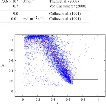
The light distribution model requires a separation between direct and diffuse light. Observations of the diffuse flux were not available for the study period, but observations of the dif-fuse and total shortwave fluxes were available for June 2004 till December 2010. The latter were used to reparameterise a relationship between the diffuse fraction (fdif, the ratio
be-tween diffuse and global radiation at the surface) and the fraction of the top-of-atmosphere flux that is transmitted through the atmosphere (ftrans, the ratio between the global
Table 1.Parameter values for the photosynthesis-stomatal conductance model.
Parameter Symbol Value Unit Reference
Maximum rate of electron transport at 298 K Jmax 144.×10−6 mol m−2s−1 Thum et al. (2008)
Maximum rate of Rubisco activity at 298 K Vc,max 25.4×10⁻⁶ mol m−2s−1 Thum et al. (2008)
Activation energy for electron transport E(J ) 88.0×10³ J mol−1 Thum et al. (2008)
Activation energy for Rubisco activity E(Vc) 73.6×10³ J mol−1 Thum et al. (2008)
Empirical curvature factor θ 0.7 Von Caemmerer (2000)
Slope in stomatal conductance equation k 9.0 Collatz et al. (1991)
Intercept in stomatal conductance equation b 0.01 mol m−2s−1 Collatz et al. (1991)
Therefore, the parameters describing these boundaries were optimised by maximising the coefficient of determina-tion of the funcdetermina-tion using the data for 2004–2010 (Fig. 1), resulting in the following relationship:
fdif=1 forftrans<0.27
fdif=1–18.3(ftrans−0.27)2 for 0.27≤ftrans<0.33 fdif=1.67–2.20ftrans for 0.33≤ftrans<0.65
fdif=0.23 forftrans≥0.65
(2)
Apart from the fraction of diffuse radiation, the model re-quires a distribution of the diffuse light over sky azimuth and zenith angles. For this, we applied a standard overcast sky (Monteith and Unsworth, 1990), which has no azimuthal preference for the light, for conditions under which all ra-diation is diffuse (fdif=1). For a high fraction of diffuse radiation (0.8 < fdif<1), a skylight distribution represent-ing translucent high clouds (Grant et al., 1996) was applied, which represents diffuse conditions, but which concentrates part of the skylight in the solar direction. For lower fractions of diffuse radiation (fdif≤0.8), a clear sky distribution (Har-rison and Coombes, 1988) was adopted.
The detailed light extinction model (Appendix A) requires a distribution of the light between absorption, reflection and transmission at the leaf level. For this, the fractions 0.85, 0.09 and 0.06 were used, respectively, values provided by Ross (1975) for mean green leaves.
2.2.2 Flux model
A combined photosynthesis-stomatal conductance model was constructed, similar to the algorithms used in many large-scale ecosystem models (e.g. in ORCHIDEE; Krinner et al., 2005). The model combines a Farquhar-type photo-synthesis model (Farquhar et al., 1980) with a Ball–Berry type stomatal conductance model (Ball et al., 1987). How-ever, in contrast to typical large-scale models, we treat it here as a leaf-level model, and do the upscaling from leaf level to canopy level explicitly by accounting for the heterogeneity in environmental drivers within the canopy (see Sect. 2.1.1). Leaf-level photosynthesis is simulated as the minimum of the Rubisco-limited CO2assimilation rateAc and the
0 0.2 0.4 0.6 0.8 1
0 0.2 0.4 0.6 0.8 1
fdif
ftrans
Figure 1.Relationship between the relative amount of incoming ra-diation at the surface (as a fraction of top-of-atmosphere rara-diation)
ftransand diffuse fractionfdif. Shown are data between June 2004
and December 2010. Data points with surface fractions≤0 or>1,
as well as data points with diffuse fractions<0.1 or>1.25, were
omitted. The original relationship by Spitters et al. (1986) (dashed,
R2=0.61) as well as the reparameterised relationship (full line,
R2=0.66) are displayed.
tron transport-limited CO2 assimilation rate Aj following Farquhar et al. (1980) and Von Caemmerer (2000):
A=min(Ac, Aj) (3)
Because of the comparison with the NEE-derived photosyn-thesis flux, which has all respiration components subtracted, there is no accounting for the leaf’s dark respiration in the computation ofAcorAj.
The Rubisco-limited rateAcis simulated as a function of
CO2 concentration and O2 concentration with temperature-dependent Michaelis–Menten constants for carboxylation and oxygenation (Von Caemmerer, 2000), and is dependent on the maximum Rubisco rateVc,max(Table 1):
Ac=
(Ci−Ŵ∗)Vc,max
Ci+Kc(1+KOo)
. (4)
Here, Ci is the leaf-internal CO2 concentration, O is the
Table 2.Overview of the simulations performed for this study.
Abbreviation Description PAR CO2 Temperature Humidity
Reference simulation
HET Full heterogeneity simulation Profile Profile Profile Profile
Homogeneous conditions for one parameter
HOM_PAR Homogeneous PAR Canopy average Profile Profile Profile
HOM_PAR_LAYER Profile, but homogeneous PAR within layer Layer-averaged profile Profile Profile Profile HOM_CO2 Homogeneous CO2(canopy average) Profile Canopy average Profile Profile HOM_CO2_AC Homogeneous CO2(above-canopy
concen-tration, 28.0 m)
Profile Above-canopy Profile Profile
HOM_TEM Homogeneous temperature Profile Profile Above-canopy Profile
HOM_HUM Homogeneous humidity Profile Profile Profile Canopy average
HOM_HUM_AC Homogeneous humidity (above-canopy concentration, 28.0 m)
Profile Profile Profile Above-canopy
HOM_HUM_IC Homogeneous humidity (within-canopy concentration, 8.5 m)
Profile Profile Profile Within-canopy
Homogeneous conditions for all parameters except one
HET_PAR Homogeneous in canopy except for PAR Profile Canopy average Canopy average Canopy average HET_CO2 Homogeneous in canopy except for CO2 Canopy average Profile Canopy average Canopy average HET_TEM Homogeneous in canopy except for
temper-ature
Canopy average Canopy average Profile Canopy average
HET_HUM Homogeneous in canopy except for humid-ity
Canopy average Canopy average Canopy average Profile
Diurnally averaged conditions for all parameters except one
DHET_PAR Homogeneous in diurnal cycle except for PAR
Profile Diurnally averaged profile Diurnally averaged profile Diurnally averaged profile
DHET_CO2 Homogeneous in diurnal cycle except for CO2
Diurnally averaged profile Profile Diurnally averaged profile Diurnally averaged profile
DHET_TEM Homogeneous in diurnal cycle except for temperature
Diurnally averaged profile Diurnally averaged profile Profile Diurnally averaged profile
DHET_HUM Homogeneous in diurnal cycle except for humidity
Diurnally averaged profile Diurnally averaged profile Diurnally averaged profile Profile
Annually averaged conditions for all parameters except one
AHET_PAR Homogeneous in annual cycle except for PAR
Profile Annually averaged profile Annually averaged profile Annually averaged profile
AHET_CO2 Homogeneous in annual cycle except for CO2
Annually averaged profile Profile Annually averaged profile Annually averaged profile
AHET_TEM Homogeneous in annual cycle except for temperature
Annually averaged profile Annually averaged profile Profile Annually averaged profile
AHET_HUM Homogeneous in annual cycle except for humidity
Annually averaged profile Annually averaged profile Annually averaged profile Profile
Ŵ∗ is the CO2 compensation point, andKc andKoare the
Michaelis–Menten constants for carboxylation and oxygena-tion, respectively, which are temperature dependent (Von Caemmerer, 2000). The electron transport-limited CO2 as-similation rate Aj depends primarily on the electron
trans-port rate J at the leaf level, as well as on the leaf-internal CO2concentration (Von Caemmerer, 2000):
Aj=(Ci−Ŵ∗)J 4Ci+8Ŵ∗
. (5)
The electron transport rateJ is determined from the empiri-cal function describingJ as a function of the absorbed irra-dianceI (corrected for spectral quality and leaf absorbance) and the maximum electron transport rateJmax(Table 1),
ap-plying an empirical curvature factorθ(Farquhar et al., 1980; Von Caemmerer, 2000):
J =I+Jmax− p
(I+Jmax)2−4θ I Jmax
2θ . (6)
The photosynthetic parameters determined by Thum et al. (2008), who used stand-scale eddy covariance measurements from Norunda for 2001 to parameterise their model, were adopted (Table 1).
Leaf-level stomatal conductance,gs, is simulated follow-ing Ball et al. (1987) with a modification by Collatz et al. (1991) as a function of the CO2assimilation rate, leaf sur-face CO2concentrationcsand leaf surface relative humidity hs:
gs=b+kA hs
cs . (7)
The values for the interceptband the dimensionless slopek in this relationship are taken from Collatz et al. (1991) (Ta-ble 1). The leaf’s aerodynamic conductance,gb, is described as a function of leaf size and wind speed, following Goudri-aan (1977).
by the leaf-internal CO2concentration and thus by stomatal conductance) is determined iteratively by solving a squared function of the stomatal conductancegsapplying bisection.
The transpiration flux E is computed from the gradient between the water vapour concentrations in the stomata (as-sumed to be saturated,Hi) and the outside air (Ha) using the stomatal and aerodynamic resistances for water vapour (de-noted asg′
sandgb′, respectively) in series:
E=(Hi−Ha)(g′ s+g′
b). (8)
Driving variables for the model are PAR, CO2concentration, humidity, temperature and wind speed. The model applies the simulated distributions of light (Sect. 2.2.1) and the ob-served vertical profiles of CO2, humidity, temperature and
wind speed (Sect. 2.1.1). The observed vertical distribution of leaf area (Sect. 2.3) was used to integrate the leaf-scale photosynthesis and transpiration rates into the stand scale. 2.3 Simulation set-up
The photosynthesis-stomatal conductance model described above was applied to simulate leaf-level photosynthesis and transpiration in the canopy of the Norunda forest site. To do so, the canopy was distributed in 25 vertical layers of 1 m thickness, to which leaf density was prescribed according to the LAI profile for the site derived from the vertical leaf area distribution in the tree crowns (Morén et al., 2000) combined with an extensive stratified sampling of tree heights and tree crown lengths (Håkansson and Körling, 2002). Within these layers, the sunlit and shaded parts of the needles were sepa-rated as described above, and within each of these two frac-tions, a spherical leaf angle distribution was represented by 4×4 leaf normal azimuth and zenith angles. These 16 leaf angle classes were distributed over the hemisphere so that each of the 16 classes represents an equal fraction (1/16) of the full distribution.
The light distribution model (Sect. 2.2.1 and Appendix A) was applied to simulate the leaf-level absorption of photo-synthetically active radiation (PAR). For each layer, the con-centrations of water vapour and CO2, as well as the
tempera-ture and wind speed, were obtained from linear interpolation of the within-canopy measurements (Sect. 2.1.1). These con-ditions varied between the layers, whereas the different leaf angle classes within one layer were considered to have the same temperature, wind speed and atmospheric concentra-tions of CO2and H2O. Because of the varying PAR between the classes, stomatal conductance, and thereby leaf-internal CO2concentration, were able to vary between these as well. Apart from these simulations in which the heterogeneity within the canopy was represented explicitly (hereafter re-ferred to as simulation HET), a number of simulations were performed in which these conditions were averaged spa-tially, thereby removing part of the vertical heterogeneity. For these simulations, the conditions were prescribed to the (LAI-weighted) canopy average instead of the distribution,
or in some cases to the above-canopy (h=28.0 m) or within-canopy (h=8.5 m) value. A complete overview of the simu-lations performed in this study is given in Table 2.
Moreover, the importance of vertical heterogeneity in forc-ing parameters was compared with the annual and diurnal variability in the forcing with the help of two sets of sim-ulations in which this temporal variability was artificially removed for all parameters except one. These simulations were driven without annual heterogeneity (labelled as AHET in Table 2, applying an annually averaged vertical profile and diurnal cycle) for all parameters except one. Similarly, the simulations without diurnal heterogeneity (labelled as DHET, applying average daily conditions while maintaining the annual cycle and vertical profile) had the diurnal hetero-geneity removed for all parameters except one. The simu-lated temporally varying vertical profiles of CO2assimilation and transpiration were averaged per day and integrated over the canopy (AHET), averaged per half-hourly period of the day and integrated over the canopy (DHET), or averaged over both days and hours for each layer in the profile (HET), and the distributions (presented as percentiles) were computed.
3 Results
3.1 Comparison with observations
Photosynthesis and transpiration from the simulation in which the heterogeneity was accounted for (HET, Table 2) were compared with the photosynthesis derived from the ob-served CO2 flux and with the observed H2O flux, respec-tively, for the years 1999–2002.
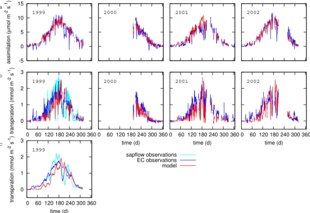
The annual cycle of photosynthesis (Fig. 2a) was generally well captured by the model. The day-to-day variability was represented, with individual days with low photosynthesis re-sulting primarily from low incoming radiation on these days (not shown). A marked decrease in photosynthesis was ob-served for a 2 week period in 1999 starting from 28 July (days 209–223), likely as a result of a preceding period of drought, coinciding with low soil moisture values (not shown; Lager-gren and Lindroth, 2002). This decrease was not captured by the model, because the impact of soil moisture conditions is not accounted for. The diurnal cycle for photosynthesis (Fig. 3a) was captured well by the model for all seasons, ex-cept for winter, when the model considerably overestimated photosynthesis. A similar 2 week drought occurred in 2001, starting at the end of June (Fig. 2a).
The annual cycle of transpiration (Fig. 2b) showed a rea-sonable agreement with the observed H2O flux (which con-sists of both evaporation and transpiration). In general, the observed flux was considerably higher than the simulated one in winter and spring (February–June), which can likely be attributed to a high contribution of evaporation to the H2O flux in spring, coinciding with the snow melt period.
-5 0 5 10 15
assimilation (
µ
mol m
-2 s -1)
a
1999 2000 2001 2002
0 1 2 3
0 60 120 180 240 300 360
transpiration (mmol m
-2 s -1)
b
1999
0 60 120 180 240 300 360 time (d)
2000
0 60 120 180 240 300 360 time (d)
2001
0 60 120 180 240 300 360 time (d)
2002
0 1 2 3
0 60 120 180 240 300 360
transpiration (mmol m
-2 s -1)
time (d)
c
1999
sapflow observations EC observations model
Figure 2.Annual cycle of simulated and observed daily mean(a)CO2assimilation and(b)transpiration for the years 1999–2002. Note that the photosynthesis parameterisation was based on observations from 2001 (Thum et al., 2008). Days with fewer than 45 (out of 48)
half-hourly observations were omitted.(c)10 day running mean of simulated and observed daily mean transpiration for 1999.
-5 0 5 10 15 20
0 6 12 18
assimilation (
µ
mol m
-2 s -1)
a MAM
0 6 12 18
JJA
0 6 12 18
SON
0 6 12 18 24
DJF
0 1 2 3
0 6 12 18
transpiration (mmol m
-2 s -1)
b MAM
0 6 12 18
JJA
0 6 12 18
time (h)
SON
0 6 12 18 24
DJF
observations model
Figure 3.Diurnal cycle of simulated and observed(a)CO2
assim-ilation and (b)transpiration, averaged for four seasons with data
from 1999, 2000 and 2002.
(applying the tissue heat balance method, Lagergren and Lin-droth, 2002) showed a later onset of transpiration (Fig. 2b and c), in better agreement with the simulated rates. The di-urnal cycle of transpiration (Fig. 3b) showed this overesti-mation for winter and spring in the daytime, with a particular mismatch for the winter season, when simulated transpira-tion was negligible. For summer and autumn, however, the
average diurnal cycle was captured well by the model, with a slight underestimation between 6 a.m. and noon.
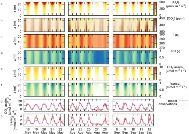
Three 5 day periods were selected as case studies (Fig. 4), which are analysed below with respect to their within-canopy variations under environmental conditions (Fig. 4a–d). Case 1 (18–22 May 1999) was selected to represent large within-canopy gradients of humidity and temperature. Case 2 (24– 28 August 1999) represents large changes in sky conditions, and therefore large changes in the vertical distribution of light. Case 3 (8–12 September 1999) exhibits large gradi-ents of atmospheric CO2 concentration within the canopy. For these cases, the dynamics of canopy-scale photosynthe-sis and transpiration (Fig. 4g and h) were captured well by the simulation model. Negative fluxes of CO2assimilation in
the observations (Fig. 4g) are due to the method used to sep-arate the net CO2flux into CO2assimilation and ecosystem
respiration, and represent the noise in the observation-based flux.
Figure 4.Overview of vertical gradients in the canopy for three periods: 18–22 May 1999 (case 1), 24–28 August 1999 (case 2) and 8–12
September 1999 (case 3). Shown are gradients of(a)leaf-level absorbed photosynthetically active radiation (PAR), averaged per canopy layer,
(b)atmospheric CO2concentration,(c)air temperature,(d)relative humidity,(e)simulated CO2assimilation and(f)simulated transpiration,
as well as the canopy-integrated(g)CO2assimilation and(h)transpiration, compared with observed fluxes (the canopy-integrated fluxes
in(g)and(h)are expressed per ground area). The gradient in PAR originates from detailed simulation of the light transfer in the canopy.
Gradients in CO2, air temperature and relative humidity were obtained from linear interpolation of measurements at 5–6 levels in and directly
above the canopy.
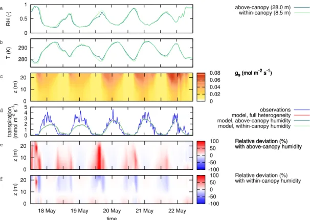
3.2 Heterogeneity in humidity and temperature For the period of the first case study, 18–22 May 1999, the CO2 assimilation flux was captured well by the model
(Fig. 4g), and the simulated transpiration flux was slightly underestimated for 18 and 19 May, whereas it was captured well for 20–22 May (Fig. 4h). During this 5 day period, there were marked differences between the conditions above the canopy and within the canopy (Fig. 5). In general, temper-atures were up to 3 K higher above the canopy than within, and relative humidity was up to 15 % lower. Differences were largest during nighttime, e.g. in the nights between 18 and 19 and between 19 and 20 May (Fig. 5a and b), but even in the early morning and late evening, while photosynthe-sis occurred, differences were apparent. The pattern of stom-atal conductance (Fig. 5c) followed primarily that of photo-synthesis (Fig. 4e), which is the main cause of the similar-ity in the vertical profiles of photosynthesis and transpiration (Fig. 4f).
Variations in relative humidity have two opposing effects: (1) a high relative humidity causes the stomatal conductance to be high (Eq. 7) and thereby stimulates transpiration and
CO2 assimilation, and (2) under high relative humidity, the
humidity gradient between the substomatal cavity (which is assumed to be saturated) and the air surrounding the leaf is low, thereby hampering transpiration.
The simulation with homogeneous temperature (HOM_TEM) or humidity (HOM_HUM) resulted in very similar CO2 assimilation and transpiration compared
0 0.5 1
RH (-)
a above-canopy (28.0 m)
within-canopy (8.5 m)
280 290
T (K)
b
c gs (mol m
-2 s-1)
0 10 20
z (m)
0 0.02 0.04 0.06 0.08
0 1 2 3 4 5
transpiration (mmol m -2 s -1)
d
gs (mol m-2 s-1)
observations model, full heterogeneity model, above-canopy humidity model, within-canopy humidity
e
gs (mol m-2 s-1)
Relative deviation (%) with above-canopy humidity
0 10 20
z (m)
-100 -50 0 50 100
f
gs (mol m-2 s-1)
Relative deviation (%) with above-canopy humidity
Relative deviation (%) with within-canopy humidity
18 May 19 May 20 May 21 May 22 May
time 0
10 20
z (m)
-100 -50 0 50 100
Figure 5.Effect of temperature and humidity conditions on transpiration for the case period 18 to 22 May 1999:(a)above-canopy (28.0 m)
and within-canopy (8.5 m) relative humidity;(b)above-canopy and within-canopy temperature;(c)simulated profile of stomatal conductance,
averaged per layer;(d)simulated transpiration, as well as observed H2O flux;(e)relative deviation in simulated transpiration when
apply-ing above-canopy humidity (simulation HOM_HUM_AC);(f)relative deviation in simulated transpiration when applying within-canopy
humidity (simulation HOM_HUM_IC).
to 20 May). Applying the above-canopy conditions yielded reasonable results in the top of the canopy, but overesti-mated transpiration in the lower canopy (Fig. 5e). The use of within-canopy humidity caused reasonable results for the lower canopy (with no deviations for the actual height of the measurements, 8.5 m), but with the top of the canopy depict-ing an underestimation of transpiration (Fig. 5f). From the two opposing effects mentioned above, the changes in hu-midity gradient were driving these deviations, whereas the stomatal response had only a mild counteracting effect.
The deviations can be considerable during the period with little or no daylight, but the difference disappeared during daytime. Hence, the daily total transpiration was only slightly affected, with 7 days exceeding an overestimation of 10 % in the period April–September for the simulation with above-canopy humidity, and 7 days exceeding an underestimation of 10 % for the same period for the simulation with within-canopy humidity. On an annual basis, the total overestima-tion of the annual transpiraoverestima-tion was 1.0 % in the simulaoverestima-tion with above-canopy humidity, and the underestimation was 1.6 % in the simulation with within-canopy humidity (not shown). Effects of above-canopy or within-canopy temper-ature rather than the tempertemper-ature average yielded even lower deviations in the simulated transpiration (not shown): an
un-derestimation of 0.5 % when using above-canopy ture, and no difference when using within-canopy tempera-ture. Because the changes in stomatal conductance were only minor, the simulated CO2assimilation flux was affected less than the transpiration flux.
3.3 Heterogeneity in light absorption
Within-canopy heterogeneous light conditions were the most important contribution to the within-canopy heterogeneity of the simulated photosynthesis and transpiration rates. The case study period 24–28 August 1999 (Fig. 4) showed a marked difference in the vertical profiles of light absorption (Fig. 4a), photosynthesis (Fig. 4e) and transpiration (Fig. 4f) between clear days (e.g. 25 August) and overcast days (e.g. 27 August), resulting in canopy photosynthesis rates that dif-fer greatly (Fig. 4g). These difdif-ferences were largely caused by the absolute amounts of radiation.
0 500 1000 1500
PAR
(
µ
mol m
-2 s -1)
a diffuse radiation
direct radiation
b LUE (-)
0 10 20
z (m)
0 0.02 0.04 0.06 0.08
c
LUE (-)
LUE (-)
0 10 20
z (m)
0 0.02 0.04 0.06 0.08
d
LUE (-)
LUE (-)
LUE (-)
0 10 20
z (m)
0 0.02 0.04 0.06 0.08
0 0.05 0.1
24 Aug 25 Aug 26 Aug 27 Aug 28 Aug
LUE (-)
time
e
LUE (-)
LUE (-)
LUE (-)
full heterogeneity layering average light conditions
Figure 6.Light conditions and their distribution in the canopy for the case period 24 to 28 August 1999:(a)above-canopy photosynthetically
active radiation (PAR, separated into direct and diffuse components);(b)light use efficiency (LUE, CO2assimilation per unit of absorbed
PAR) for the full heterogeneity case (simulation HET);(c)light use efficiency for a set-up that does not separate sunlit and shaded leaves
(simulation HOM_PAR_LAYER);(d)light use efficiency for a set-up that separates neither sunlit and shaded leaves, nor layers (simulation
HOM_PAR);(e)canopy-scale light use efficiency (CO2assimilation per unit of incoming PAR).
of direct radiation, part of the canopy is light-saturated and produces at its maximum rate. However, a large part of the canopy, most notably the shaded leaves, receive consider-ably lower amounts of radiation. In contrast, for overcast conditions, e.g. those prevailing on 27 August, the light is distributed more evenly in the canopy. This, combined with the generally lower level of radiation, makes that less leaves are under light-saturated conditions, and that the lower part of the canopy receives more light and is contributing more to the canopy photosynthesis.
The impact of sky conditions on the distribution of the light affected the light use efficiency (LUE, which is defined here as the CO2 assimilation flux per amount of absorbed
PAR) of the canopy, both within the vertical profile (Fig. 6b) and for the canopy as a whole (Fig. 6e). Around noon on sun-lit days, the absorption in the top of the canopy was high, and the LUE in the top of the canopy was low, resulting in lower canopy LUE values (Fig. 6e). In the early morning and late evening hours of clear-sky days, as well as on overcast days, the fraction of diffuse radiation was high and the absolute amount of incoming PAR was low, resulting in a more even distribution of the light in the canopy, and generally lower photosynthesis rates. In contrast to the low absolute amounts, the efficiency was higher, which resulted in improved canopy LUE.
The light extinction scheme applied here distinguishes leaf-level heterogeneity in light absorption caused by the dis-tinction between sunlit and shaded leaves, the vertical lay-ering of the canopy and the distribution of leaf angles. The contribution of these factors to the heterogeneity in CO2 as-similation, and thereby their impact on LUE, is illustrated in Fig. 6b–d. Simulation HOM_PAR_LAYER, which did not separate sunlit and shaded leaves or leaf angles, and which obtains its heterogeneity only from the layering in the canopy, had uniform conditions within the vertical lay-ers, and represents a light extinction scheme that does not account for sunlit-shaded leaves, as is often applied in large-scale models. It resulted in considerably higher LUE values (Fig. 6c), particularly in the lower part of the canopy, where the distinction between sunlit and shaded leaves results in a small proportion with high PAR levels and a large propor-tion with very low levels. An even more equal distribupropor-tion of the light was obtained with simulation HOM_PAR (Fig. 6d), which had no layering in the canopy either. This represents the so-called big-leaf approach, as used in large-scale mod-els that lack a vertical layering. It resulted in a homogeneous distribution of the light, and in the highest LUE values for the canopy (Fig. 6e).
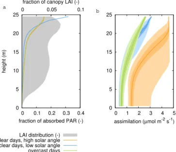
0 5 10 15 20 25
0 0.1 0.2 0.3 0.4
0 0.05 0.1
height (m)
fraction of absorbed PAR (-)
a
fraction of canopy LAI (-)
LAI distribution (-) clear days, high solar angle clear days, low solar angle overcast days
0 5 10 15 20 25
0 1 2 3 4 5
assimilation (µmol m-2 s-1)
b
Figure 7.Vertical distribution of(a)light absorption and(b)CO2
assimilation in the canopy (expressed per leaf area), separated for clear time steps (fdif<0.5) with a solar angleβ >30◦(n=1418),
clear time steps with a solar angleβ <30◦(n
=1382), and cloudy
time steps (fdif≥0.5,n=4888) for 1999. The average
distribu-tion within a layer in(b) is represented by the median, 25–75 %
percentile, and 5–95 % percentile.
distribution were important contributions to the within-canopy heterogeneity. Apart from the generally higher levels of radiation and hence CO2assimilation obtained under high solar angles, the radiation penetrated deeper into the canopy, resulting in a more even distribution of the radiation (Fig. 7a) and higher levels of CO2 assimilation further down in the canopy (Fig. 7b) compared to cases with a low solar angle. Similarly, the high levels of diffuse radiation obtained under overcast conditions resulted in a more homogeneous distribu-tion of the light because of the contribudistribu-tions from different azimuth and zenith angles, resulting in a more even vertical distribution of CO2assimilation (Fig. 7).
This profound difference between clear and overcast con-ditions was obtained as well when separating the daily CO2
assimilation flux over clear days (defined here as days with more than 50 % of the radiation reaching the canopy directly) and cloudy days (less than 50 % of the radiation reaching the canopy directly): for clear days, lower efficiencies in CO2 assimilation with a given amount of light (Fig. 8) were ob-tained; the light use efficiency is depicted here as the slope in the figure. The model set-up depicting the full distribu-tion of light in the canopy (simuladistribu-tion HET) was able to cap-ture the efficiency for both the clear days and cloudy days, and showed a marked difference between the two. The set-up without heterogeneity in the canopy light distribution (sim-ulation HOM_PAR) generally overestimated the efficiency because of the equal distribution of light. Moreover, the dif-ference in light use efficiency between clear days and cloudy
days was smaller. The model set-up used for HOM_PAR did not differentiate between direct and diffuse radiation, but the regression still depicted a difference because of the relative importance of high PAR days to the clear day set, which gen-erally show a lower efficiency.
On the annual scale, GPP was captured well by the sim-ulation applying full heterogeneity (simsim-ulation HET), with a slight overestimation of 3 % of the annual GPP compared with the observations for the days for which data are avail-able. The simulation without heterogeneity in the light distri-bution (HOM_PAR) overestimated GPP by 44 % compared to this full heterogeneity set-up, whereas the simulation with a layering only (HOM_PAR_LAYER) overestimated GPP by 14 %.
3.4 Heterogeneity in CO2concentration
Within the canopy, the ambient concentration of CO2 can vary considerably, both in time and in the vertical (Fig. 4b). Large gradients are formed under stable conditions dur-ing nighttime, when CO2assimilation has stopped, but het-erotrophic and autotrophic respiration continue, while verti-cal mixing is reduced in the canopy. These gradients disap-pear quickly after sunrise, when the boundary layer growth starts and initiates turbulent mixing. It is mainly during these early morning hours that effects of a CO2 gradient in the
canopy on fluxes of CO2assimilation and transpiration were
to be expected.
These large gradients were seen in the third case period (Fig. 4b), and we will illustrate this impact by analysing the dynamics of this gradient on 12 September 1999 in more detail (Fig. 9). For this date, the CO2 gradient built up during nighttime, and a gradient of more than 50 ppm was maintained up to two hours after sunrise (Fig. 9c). Ig-noring this gradient in the simulation of CO2 assimilation by using a constant (canopy-average or above-canopy) CO2 concentration caused deviations of a few percents locally (Fig. 9d), but its impact on the actual profile (Fig. 9e), or on the canopy-integrated CO2assimilation flux was negligible.
From 8.30 a.m. onwards, the gradient disappeared rapidly, and had no further impact on CO2 assimilation during the
day (Fig. 9c–e).
Despite the substantial gradient in CO2concentration, its
0 5 10 15 20
0 100 200 300 400 500 600 700
assimilation (
µ
mol m
-2 s -1 )
PAR (µmol m-2 s-1)
data (clear days) data (cloudy days) model (clear days) model (cloudy days) model w/o heterogeneity (clear days) model w/o heterogeneity (cloudy days)
A = 0.013 PAR (R2=0.68; n=80) A = 0.019 PAR (R2=0.91; n=107) A = 0.013 PAR (R2=0.82; n=122) A = 0.019 PAR (R2=0.86; n=155) A = 0.020 PAR (R2=0.74; n=122) A = 0.026 PAR (R2=0.84; n=155)
Figure 8.Daily integrated flux of CO2assimilation as a function of the daily integrated photosynthetically active radiation (PAR) separated
for clear days (fdif<0.5) and cloudy days (fdif≥0.5). Shown are results from the full heterogeneity simulation and the simulation without
heterogeneity in light, as well as the observation-derived CO2assimilation flux. Days with fewer than 45 (out of 48) half-hourly observations
were omitted. Regression lines (obtained with least-squares linear regression through the origin) are shown for the three data sets as well (full lines corresponding to the clear days, dashed lines to the cloudy days).
photosynthesis is underestimated in the lower canopy, the simulations yield an underestimation of transpiration as well because of the lower CO2concentration (not shown).
How-ever, similarly to the impact on photosynthesis, the change in transpiration had only a marginal impact, and occured where and when transpiration rates were small anyway.
The occurrence of CO2 gradients, predominantly during nighttime and morning hours, has therefore a negligible im-pact on canopy-integrated photosynthesis levels.
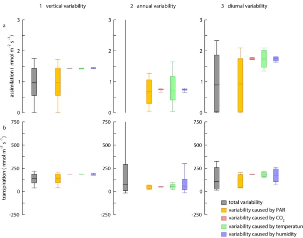
3.5 Comparison with annual and diurnal heterogeneity The analysis above showed the vast dominance of light as the cause of within-canopy heterogeneity of CO2
assimila-tion and transpiraassimila-tion. A set of simulaassimila-tions that were forced by within-canopy heterogeneity of only one of the driving parameters (PAR, CO2, temperature and humidity,
simula-tions HET_PAR, HET_CO2, HET_TEM and HET_HUM) illustrates this: Fig. 10a1 and b1 compare the observed vari-ability in CO2 assimilation and transpiration fluxes within the canopy between the full heterogeneity simulation (HET) and the set of partial heterogeneity simulations. It clearly shows that the simulation in which light was the only het-erogeneous variable (HET_PAR) had comparable variability for both CO2assimilation and transpiration fluxes, whereas the other simulations had a much smaller variability.
In order to compare the importance of vertical heterogene-ity with that obtained from annual and diurnal changes in the forcing, the variability was determined on the annual and
diurnal scale for the two additional sets of simulations in which annual and diurnal heterogeneity in the forcing were removed, respectively. Figure 10a2 shows that the annual variability in the flux of CO2 assimilation is determined in
equal amounts by variations in PAR and temperature. For the annual variability in transpiration, variability in humid-ity played a dominant role, with minor contributions from PAR and temperature as well (Fig. 10b2).
The diurnal variability of the CO2 assimilation flux was largely dominated by PAR (Fig. 10a3), which is the obvious driver of the daytime-to-nighttime difference in CO2 assimi-lation. Moreover, temperature contributed to the diurnal vari-ability as well. For diurnal variations in transpiration, PAR and humidity changes played equal roles (Fig. 10b3).
Summarising, the within-canopy variability in fluxes of CO2 assimilation and transpiration was of a similar order
of magnitude as the variability on annual or diurnal scales (Fig. 10), though typically slightly less than the latter. PAR-related variability within the canopy was of a similar magni-tude as the PAR-related variability at the annual cycle.
4 Discussion
For the evaluation of the model, gross primary produc-tion (GPP) was derived from the CO2 flux determined
0 6 12 18 24 0
500 1000 1500
PAR (µmol m -2 s
-1 )
PAR
0 6 12 18 24350
360 370 380 390
CO
2
conc. (ppm)
CO2
0 6 12 18 24
time (h) 0
10 20
CO
2
assim.
(
µ
mol m
-2 s
-1 )
observations model
360 440 0
10 20
height (m)
360 440 360 440 360 440 360 440
CO2 conc. (ppm)
360 440 360 440 360 440 360 440
0.96 1.04 0
10 20
height (m)
0.96 1.04 0.96 1.04 relative assim. (-)
0.96 1.04 0.96 1.04 0.96 1.04
0 2 4 0 10 20
height (m)
simulation applying CO2 profile
simulation applying average CO2
simulation applying
above-canopy CO2 0 2 4 0 2 4
assim. (µmol m-2 s-1)
0 2 4 0 2 4 0 2 4
(a)
(b)
(c)
(d)
(e)
05:00 am 06:00 am 07:00 am 08:00 am 09:00 am 10:00 am 1:00 pm 4:00 pm 9:00 pm
Figure 9.Changes in the within-canopy CO2profile, and its impact on CO2assimilation, illustrated for 12 September 1999:(a)observed
changes in PAR and above-canopy (28 m) CO2concentration;(b)simulated and observation-derived CO2assimilation;(c)within-canopy
CO2profile for nine selected times;(d)relative deviations from simulated CO2assimilation when applying average (simulation HOM_CO2)
or above-canopy (simulation HOM_CO2_AC) CO2concentrations instead of the distribution displayed in(c);(e)simulated CO2assimilation
for simulations applying the CO2distribution as well as canopy-average or above-canopy CO2concentration. For(d)and(e), only daytime
panels were shown.
temperature dependence. Moreover, the comparison between the simulated canopy-scale transpiration and the H2O flux
determined with eddy covariance showed large deviations in winter and spring, most likely caused by the contribu-tion of evaporacontribu-tion to the flux, as supported by the improved comparison between model and observations obtained with sapflow measurements (Lagergren and Lindroth, 2002). Un-fortunately, sapflow measurements were available only for a nearby (distance approximately 500 m) site, and not for all years used in the model evaluation.
The model simulated CO2assimilation and transpiration
fluxes as a function of atmospheric conditions, but did not account for soil conditions. Soil moisture limitations may af-fect the stomatal conductance, and thereby the fluxes of CO2
assimilation and transpiration. Such water limitation occa-sionally occurred in the forest site studied here, mainly dur-ing summertime and for periods of up to 15 days (Jansson et al., 1999; Grelle et al., 1999; Lagergren and Lindroth, 2002; Thum et al., 2007), but the non-water limited results are representative of this site for most of the year. For other sites, it may be considerably more important to capture this response.
Despite these drawbacks, simulated and observed CO2 as-similation fluxes showed a good agreement, and simulated transpiration showed a reasonable agreement with the ob-served evapotranspiration.
Figure 10.Explanation of variability of simulated(a)CO2assimilation and(b)transpiration for(1)vertical variability (n=25),(2)annual
variability (n=277) and(3)diurnal variability (n=48). Shown are the distributions (box indicates the median and the 25–75 % percentile,
whiskers indicate full distribution) obtained from the full simulation, and from simulations that exhibit variability only for one parameter (see text for details).
canopy, and showed that the vertical distribution of photo-synthetically active radiation is the dominating source of ver-tical heterogeneity. The importance of sky conditions for the flux of CO2assimilation has been studied in other coniferous
forests. Considerably higher photosynthetic light use effi-ciency, and thereby a stronger net carbon sink, was observed for cloudy days as compared with clear days for aPicea abies
stand in the Czech Republic (Urban et al., 2007), for two
Picea sitchensisstands in the UK (Dengel and Grace, 2010),
and for aPinus sylvestrisstand in Finland (Law et al., 2002),
in agreement with the results presented in this study. Stomatal conductance was observed to be larger for cloudy conditions than for clear conditions (Dengel and Grace, 2010), for which the enhancement of light absorption and thereby photosynthesis is only one possible explanation: In general, cloudy conditions coincide with a relatively low vapour pressure deficit, which enhances stomatal conduc-tance as well. Our results suggest that this is of little impor-tance for the diurnal dynamics of photosynthesis, but it may be more important for the seasonal dynamics (as addressed by Dengel and Grace, 2010). Moreover, the higher contri-bution of blue light to the radiation under diffuse conditions has been suggested as an explanation for higher conductance
(Dengel and Grace, 2010), but this was not confirmed for thePicea abiesstand in Czech republic (Urban et al., 2012).
These effects of spectral differences cannot be studied with our model in its current form, but may be interesting for fu-ture model development.
Variability within the CO2 profile had little effect on the simulated canopy CO2 assimilation rates in this study, mainly due to the counteracting effects of changes in ambi-ent CO2 and changes in stomatal conductance (and thereby leaf-internal CO2). Brooks et al. (1997) estimated an increase of 5–6 % in understorey CO2assimilation due to the elevated
levels of CO2resulting from respiration for two boreal
for-est sites in Canada. However, the understorey is not likely to contribute substantially to the canopy GPP. Rough estimates of ground vegetation net primary production for this site (un-published results) indicate a contribution of less than 10% to the total, which is in the range obtained for other Swedish forest sites (Berggren et al., 2002). We expect the contribu-tion to GPP to be of similar magnitude.
temperature measurements in a number of layers, and is thus not entirely representative of leaf temperatures. Importantly, leaf temperatures are affected by fluxes of radiation, and sun-lit and shaded leaves may thus exhibit different temperatures. Observations of individual leaf temperatures, and their dis-tribution in the canopy, are rare, and in order to investigate the importance of temperatures further, a leaf energy balance model may be used to compute temperatures.
Apart from the variations in the environmental driving variables, variations can occur in model parameters as well. The vertical gradient in light availability causes plants to dis-tribute the leaf nitrogen content, and thereby the photosyn-thetic capacity, with a similar vertical gradient (Hirose and Werger, 1987; Givnish, 1988); in models this effect is of-ten translated into an assumed optimum vertical distribution of nitrogen and photosynthetic capacity (De Pury and Far-quhar, 1997). We have performed sensitivity tests applying an exponentially decreasingVc,maxas suggested by De Pury
and Farquhar (1997), resulting in an enhanced vertical gradi-ent in CO2assimilation under all sky conditions, and a fur-ther decrease in the light use efficiency. On the canopy scale, the light use was affected equally under clear or cloudy days, causing a reduction of 16 % in LUE.
Similarly, temporal variations of photosynthetic capacities occur during the growing season, which was found for the Norunda forest site as well (Thum et al., 2008). However, Op de Beeck et al. (2010) found these seasonal variations to be relatively unimportant for the simulation of net ecosystem exchange in aPinus sylvestrisforest in Belgium. Apart from the vertical heterogeneity, there is a difference in these pho-tosynthetic parameters as well between tree species. Pinus sylvestrishas been observed to have generally higher rates
of CO2assimilation thanPicea abies, both for the
Rubisco-limited (Eq. 4) and for the electron transport-Rubisco-limited (Eq. 5) regimes (e.g. Wullschleger, 1993; Thum et al., 2008). In the current model, this separation, which requires the interac-tion between two (or more) tree species to compute the light transfer, cannot be accounted for. Moreover, such a separa-tion would enhance uncertainties related to the parameterisa-tion.
5 Conclusions
The simulations of fluxes of CO2assimilation and transpira-tion for a boreal coniferous forest in central Sweden revealed that the gradient of PAR is the main driver of vertical het-erogeneity within the canopy. Because of the concave shape of the response of photosynthesis to light, averaging of PAR in the canopy resulted in an overestimation of the photosyn-thesis rate. The other driving variables tested here (tempera-ture, CO2concentration, humidity and wind speed) had little
impact on the canopy-integrated rates of photosynthesis and transpiration, and these can be well represented by a canopy-average value.
In models applied on regional or global scales, vertical heterogeneity in the driving variables is largely ignored. Whereas a canopy-average value is sufficient to represent temperature, CO2concentration and humidity, the distribu-tion of PAR needs to be represented in more detail than a big-leaf approach, a result in accordance with earlier stud-ies (Roderick et al., 2001; Alton et al., 2007; Knohl and Bal-docchi, 2008; Mercado et al., 2009). A more detailed repre-sentation in large-scale models will enable a more realistic treatment of the effects of sky conditions on photosynthesis. Given the size of the vertical variability of the fluxes of CO2assimilation and transpiration within the canopy, which
Appendix A: Description of light extinction scheme Light extinction was simulated with a numerical scheme that builds on existing theory, representing the heterogene-ity in the canopy due to sunlit and shaded fractions (which was introduced by Duncan et al., 1967), vertical layering (used for representing the vertical heterogeneity by e.g. Mon-teith, 1965; Duncan et al., 1967; Cowan, 1968) and leaf an-gle distribution (addressed with numerical approximations by Goudriaan, 1977, 1988). However, in contrast to exist-ing schemes, we refrain from averagexist-ing intermediate results (e.g. the distribution of insolation levels obtained from vary-ing leaf angles) over the canopy, so that the distribution ob-tained represents the full distribution of light at the leaf level. A1 Leaf angle distribution
Leaf orientation is represented by two dimensions: an az-imuth angle φl (0≤φl<360◦) and a zenith angle θl (0≤
θl<90◦) of the leaf normal. The distribution of leaf
orien-tation in these two dimensions is represented in a discrete manner as a lattice withnlφ×nlθ combinations of azimuth
and zenith angles. The spacing in φ andθ is done so that each combination (φl, θl) has an equal likelihood, and
repre-sents 1/(nlφnlθ)of the complete leaf area. For the
simula-tions in this study, we applied a spherical (or isotropic) leaf angle distribution, which is obtained with a uniform distribu-tion (equal spacing) of the azimuth anglesφlover the entire
360◦, and a spacing at equal distances between the cosines
of the angles for the zenith anglesθl, so that the increasing
density towards the horizon compensates for the increasing area of the sphere.
A2 Distribution of sunlight and skylight
In the model, sunlight is described as a point source with a given azimuth and zenith angleφsunandθsun, respectively, together with a photosynthetic quantum flux densityIsun(in mol m−2s−1). Similar to the leaf angles, skylight is described
with a distribution of azimuth and zenith angles over the hemisphere. In contrast to the leaf angle distribution, how-ever, azimuth and zenith angles are spaced equally, resulting in niφ×niθ combinations of (φs, θs), and the intensity for
each combination is given byIs(φs, θs). The distribution of
the light over sunlight (direct radiation) and skylight (diffuse radiation), as well as the distribution of skylight over all an-gles (φs, θs), is determined by sky conditions.
To accommodate upward scattering of light within the canopy, a second hemisphere was introduced, which has the same number and distribution of azimuth and zenith angle classes.
A3 Light absorption
The canopy is represented bynhlayers, and light absorption,
reflection and transmission in the canopy are calculated by
combining the direct radiation and the distribution of sky-light radiation over the sky angles (Sect. A2) for each of the leaf orientations (Sect. A1) in each layer, thus resulting in a probability density function of leaf-level absorbed radia-tion. Below, we will describe the processes at the leaf level first, followed by a description of the aggregation of these processes to canopy scale.
The leaf angle distribution is assumed to be spherical (or isotropic), meaning that the leaf area in layerh,Lh, is
distributed equally over all leaf angle orientations(φl, θl),
which is commonly used to describe a generic canopy in large-scale models (Cowan, 1968; Leuning et al., 1995) The leaf area was divided into a sunlit and a shaded fraction (com-putation of these fractions will be explained further down). This leaf area intercepts a fraction of the radiation that comes from a given direction(φs, θs)proportional to its area, and it
depends on the angle between the leaf normal and the direc-tion of the radiadirec-tion:
fint,s,l,h=
sinγs,l
cosθs
Lh
nlφnlθ
. (A1)
In this equation, the angle between beam and leaf,γs,l, can be
computed from the inner product of the vectors of the beam and the leaf normal, which can be expressed based on their azimuth anglesφand zenith anglesθ(see e.g. Ross, 1981): γs,l=arcsin(cosφssinθscosφlsinθl (A2)
+sinφssinθssinφlsinθl+cosθscosθl)
This intercepted fraction of the radiation,fint,s,l,h (Eq. A1)
is absorbed, reflected or transmitted by the leaf, which is distributed according to constant fractions. To obtain the to-tal amount of intercepted diffuse radiation by the leafIdif,l,h
(which represents intercepted radiation by the leaf area with orientationl in layer h), these fractions, multiplied by the light intensitiesIdif, need to be integrated over all skylight
angles:
Idif,l,h=
ns
X
s=1
(fint,s,l,hIdif,ssinγs,l). (A3)
This integration is performed both for the upper hemisphere and for the lower one to accommodate fluxes from below due to scattering.
Similarly, the fraction of intercepted beam radiation can be computed from Eq. (A1) by replacing the skylight angles with sunlight angles, which results in the beam radiation in-tercepted by a leaf with orientationlin layerhof
Isun,l,h=fint,sun,lIsunsinγsun,l. (A4)
The total amount of intercepted radiation by the leaf area with orientationl in layerh, which can be written as Isun,l,h+fsun,hIdif,l,hfor sunlit leaves, and(1−fsun,h)Idif,l,h
leaf areas, respectively, to obtain the radiation intensity at the leaf level:
Iint,sunlit,l,h=
Isun,l,h+fsun,hIdif,l,h
fsun,hnlφnlθLh
(A5)
Iint,shaded,l,h=
Idif,l,h
nlφnlθLh
(A6)
The fractions of sunlit and shaded leaves are computed from the same theory: the total interception of radiation in layerh is calculated by integrating Eq. (A1) over all leaf angles:
fint,h=
nlφnlθ
X
l=1
fint,l(φl, θl). (A7)
The fraction of sunlit leaves for each layer h is computed from the shading in the layers above, assuming the leaves to be distributed randomly in space (no spatial aggregation), similar to Monteith (1965):
fsun,h=(1−fint)h−1. (A8) This results in an exponential profile of the sunlit fraction in the canopy.
The absorbed photon flux densities at the leaf level, ob-tained from Eqs. A5 and A6, are used to compute CO2 assim-ilation (see Sect. 2.2.2). The unintercepted radiation passes the layer without adjustments to the angular distribution. The radiation transmitted and reflected is distributed again over the two hemispheres of diffuse radiation. The leaf surface is assumed to be a Lambertian scatterer: the leaf reflects the largest flux in the direction of the leaf normal, and trans-mits the largest flux in the opposite direction. When the dif-fuse light reaches the leaf surface from below, transmittance points in the direction of the leaf normal, and reflectance in the opposite direction.
These leaf-level processes can be aggregated to the canopy level. For all leaf orientationsj in all layersh, absorbance, reflectance and transmittance from the layer as a whole can be determined as described above. Within a layer, the scat-tering in all directions of the upward and downward pointing hemisphere is integrated over all leaf orientations, and these amounts are added to the fluxes of diffuse radiation that pass through the layer without interference with the leaves.
The distribution of this scattered light over the canopy is solved iteratively by computing the total absorption of both downward and upward pointing fluxes for all layers, first from top to bottom, then from bottom to top. This is repeated until the remaining scattered light within the canopy is lower than a pre-defined minimum residual (0.001 %). This way of distributing the light in the model canopy is relatively effi-cient; it requires a few iterations to reach this residual.