ANALYSIS OF HOUSEHOLD BEHAVIOUR TO THE
COLLECTION OF WASTE ELECTRICAL AND ELECTRONIC
EQUIPMENT IN ROMANIA
MARIA LOREDANA NICOLESCU
Business Administration & Marketing Department
Nicolae Titulescu University, Bucharest
ROMANIA
[email protected]
MARIUS NICOLAE JULA
Finance-Banking & Accounting Department
Nicolae Titulescu University, Bucharest
ROMANIA
[email protected]
Abstract: - This paper presents an analysis of household behaviour to the collection of waste electrical and electronic equipment in Romania based on an econometric multifactorial linear regression model. In the model, the amount of WEEE* collected in the counties represents the endogenous variable, and factors such as regional gross domestic product, the number of employees, monthly average net nominal earnings, unemployed persons, retirees, existing housing, education and other non-quantifiable factors with regional influence are influence factors or explanatory (exogenous) variables. The period considered for the study is 2010-2012, and statistics are taken and processed at county level.
The study is necessary to identify the extent to which those factors influence the collection of WEEE from private households. The results of this study may lead to an improvement of the management of waste electrical and electronic equipment in Romania, being useful for policy makers and stakeholders involved in the system.
Key-Words: waste electrical and electronic equipment (WEEE), WEEE collection, econometric modelling of household behaviour, endogenous variable, explanatory (exogenous) variables.
1. Introduction
The international scientific community believes that an optimised waste management may allow obtaining economic, social and environmental benefits (Cucchiella, D’Adamo & Gastaldi, 2014 cited in Cucchiella, D’Adamo, Koh & Rosa, 2015). Understanding consumer behaviour to the recycling of WEEE is important for decision makers in Romania to take the correct measures to meet collection targets imposed by the European Directive (Colesca, Ciocoiu & Popescu, 2014).
According to national and European statistics on waste electrical and electronic equipment (WEEE), Romania faces the problem on not fulfilling the collection target of 4 kg/capita/year from private households. High levels of WEEE, small quantities of WEEE collected, limited recycling and disposal facilities together with the need to transpose EU legislation into national law have shaped the profile of the WEEE management system in Romania (Colesca, Cocoiu & Popescu, 2014). The main problems of the WEEE management system in Romania are related to the collection process and the unregulated activity of the informal sector (Rudăreanu, Popescu, Ciocoiu & Colesca, 2015). To improve the functionality of the system it is important to understand the behaviour of citizens towards WEEE collection. They are provided with the WEEE collection service free of charge, yet the question remains: why isn’t there more waste electrical and electronic equipment collected in Romania?
WEEE collection. The research was based on European (Eurostat, 2015) and national (INS, 2015; ANPM, 2015) statistics available to Romania in the 41 counties plus Bucharest, in 2010-2012.
2. Econometric modelling of household behaviour to the collection of waste
electrical and electronic equipment
Analysing the relationship waste generation-economic development, five key factors stand out that have different contributions to increasing the amount of waste, including the decrease in natural resources: • size of the business or the economy;
• sectoral structure of the economy; • existing technological level;
• the demand of legislation on waste management;
• the policy and spending related to resource conservation and prevention of WEEE generation.
In the econometric multifactorial linear regression model, the amount of WEEE collected represent a variable dependent on several factors as independent variables in the model, all data being taken into account by counties.
The following were considered as potential influence factors of the collection of WEEE at county level: population size, size of economic activity (measured by regional GDP and number of employees), income (approximated by monthly average net nominal earning), weight of different categories such are county population (employed, unemployed, retired), existing housing, education level and other non-quantifiable factors with regional influence, considered invariants on the short-term (skills, beliefs, traditions, customs, etc.). In the case of education as an influence factor on the collection of WEEE in the model, we took into account the latest Eurostat records, namely the data from 2001 on the grouping of the population (persons) on various levels of education by Romanian counties, according to ISCED 97. The values for each level of education were calculated for the model as percentages of the total education levels. For each county we calculated the ratio between the population corresponding to each level and the total population that includes all levels of education in the respective county. The total was calculated for each level of education, which is divided by the total of the levels of education, as mentioned above. The weights were included in the model as LLE (lower level of education) and HLE (higher level of education) variables, considered “fixed individual effects” and calculated according to the methodology presented in the following.
Following the retrieval of data, we built a panel type model as follows:
weeeit = f(gdpit, populationit, housingit, employeesit, csnmnlit, unemployedit,
retireesit, educationit, efregi, εit), (1)
where
weeeit = the amount of waste electrical and electronic equipment (tons) collected in the county
i, year t (Source: data courtesy of Mrs. Brînduşa Petroaica, Directorate of Waste and Hazardous Chemical
Substances within the National Environmental Protection Agency, 05/13/2015).
gdpit = gross domestic product (mil. lei), in the county i, year t, SEC 2010 methodology, calculated according to NACE Rev. 2 (Source: INS, TEMPO online, date of accessing June 20, 2015, table CON103I_20_6_2015 - SEC 2010, calculated according to NACE Rev.2, mil. Lei).
populationit = population (number of persons) according to residence on January 1, in the county i, year t (Source: INS, TEMPO online, date of accessing June 20, 2015, table POP107A_20_6_2015).
housingit = the number of existing housing at the end of the year in the county i, year t (Source: INS, TEMPO online, date of accessing, June 20, 2015, table LOC101A_20_6_2015).
employeesit = number of employees at the end of the year in the county i, year t (Source: INS, TEMPO online, date of accessing June 15, 2015, table FOM105A_15_6_2015).
unemployedit = number of registered unemployed persons in the county i, year t (Source: INS, TEMPO online, date of accessing June 15, 2015, table SOM101B_15_6_2015).
retireesit = average number of retirees in the county i, year t (Source: INS, TEMPO online, date of accessing June 15, 2015, table PNS101D_15_6_2015).
educationit = level of education (weight in specific population) in the county i, year t (Source: Eurostat, “Population by sex, age group, educational attainment level, occupation (ISCO-88) and NUTS 3 regions”, date of accessing June 20, 2015, table “cens_01reisco”, http://appsso.eurostat.ec.europa.eu/nui/submitViewTableAction.do).
efregi = other non-quantifiable factors with regional influence, considered
invariants on the short-term (skills, beliefs, traditions, customs …), specific to the county i; εit = idiosyncratic error.
Because the behaviour related to the collection of WEEE is influenced by local factors, related to the specificity of the area, and, in general, cannot be quantified for inclusion in econometric models (latent factors), we opted for a panel-type model in differences (Jula, 2014). Specifically, we write the regression equation at time t and at time t-1:
weeeit = a0 + a1·gdpit + a2·populationit + a3·housingit + a4·employeesit + a5·csnmnlit +
+ a6·unemployedit + a7·retireesit + a8·educationit + a9,i·efregi + εit (2)
weeeit-1 = a0 + a1·gdpit-1 + a2·populationit-1 + a3·housingit-1 + a4·employeesit-1 + a5·csnmnlit-1 + a6·unemployedit-1 + a7·retireesit-1 + a8·educationit-1 + a9,i·efregi + εit-1 (3)
The following difference was calculated:
d(weeeit) = weeeit – weeeit-1, (4)
d(weeeit) = a1·d(gdpit) + a2·d(populationit) + a3·d(housingit) + a4·(employeesit) +
+ a5·d(csnmnlit) + a6·d(unemployedit) + a7·d(retireesit) + a8·d(educationit) +d(εit) (5)
because a0 is a calibration factor common to both equations and the variable efregi is invariable in time. By building a model in differences, we obtain consistent estimators, because the specification does not require the inclusion of local influential variables.
In terms of ensuring the data, a problem occurs in assessing the level of education, because such data are not routinely reported at county level, in national statistics (National Institute of Statistics), or in European statistics (Eurostat). Therefore, we opted for the following solution: we took the last records from Eurostat statistics regarding on different levels of education of population, and for each level we calculated values as percentages of the total population comprising all levels of education, and we have included them as constant values regionally. These data are grouped into the following levels in the model (Table 1):
Table 1. Levels of education
Indicator Symbol in the
model
Total Total
Preschool and primary education (levels 0 and 1) Levels 0 & 1
Lower secondary education (level 2) Level 2
Upper secondary education (level 3) Level 3
Post-secondary non-tertiary education (level 4) Level 4
First and second stage of tertiary education (levels 5 and 6) Levels 5 & 6
Unknown education Unknown
Source: data processing according to Eurostat, “Population by sex, age group, educational attainment level, occupation (ISCO-88) and NUTS 3 regions”, table cens_01reisco,
http://appsso.eurostat.ec.europa.eu/nui/submitViewTableAction.do
Note 1. Recent statistics use a classification with 8 levels.
Note 2. In Romania, lower secondary education means middle school. Upper secondary education includes secondary, vocational and apprenticeship schools. Post-secondary non-tertiary education includes post-secondary and foremen vocational education. The first and second stage of tertiary education are represented by higher and postgraduate education.
The variables were calculated as a share of total population. Based on these data, two variables were calculated:
The lower level of education (SLLE), including levels 0, 1 and 2: “No education” + “Preschool and primary education (levels 0 and 1)” + “Lower secondary education (level 2)”
The higher level of education (HLE), including levels 3, 4, 5 and 6: “Upper secondary education (level 3)” + “Post-secondary non-tertiary education (level 4)” + “First and second stage of tertiary education (levels 5 and 6)”
LLE = No education + Levels 0&1 + Level 2
HLE = Level 3 + Level 4 + Levels 5&6
The initially estimated model is:
d(weeeit) = a1·d(gdpit) + a2·d(populationit) + a3·d(housingit) + a4·(employeesit) +
+ a5·d(csnmnlit) + a6·d(unemployedit) + a7·d(retireesit) + a8·LLEi +
+ a9·HLEi + d(εit) (6)
In the terminology of panel-type models, the LLEi and HLEi variables are individual fixed effects.
In this model, the coefficient a6, which estimates the link between changes in the number of unemployed persons, d(unemployedit) and the evolution of waste electrical and electronic equipment collection, d(weeeit) is not significant econometrically (the risk associated with type I error is 0.7525, a lot higher than the standard threshold of 0.05). Therefore, we removed that variable from the model and retained the following specification:
d(weeeit) = a1·d(gdpit) + a2·d(populationit) + a3·d(housingit) + a4·(employeesit) +
+ a5·d(csnmnlit) + a7·d(retireesit) + a8·LLEi + a9·HLEi + d(εit) (7)
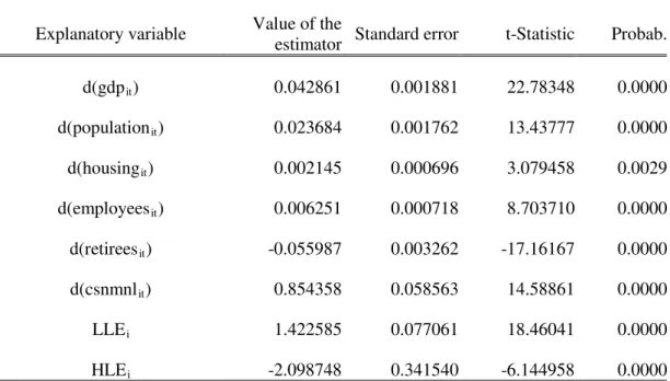
Previous model estimation results are shown in Table 2 (Dependent variable: d(weeeit); Period: 2010-2012; Number of included units: 42; Total notes: 84):
Table 2. Model estimation results
Explanatory variable Value of the
estimator Standard error t-Statistic Probab.
d(gdpit) 0.042861 0.001881 22.78348 0.0000
d(populationit) 0.023684 0.001762 13.43777 0.0000
d(housingit) 0.002145 0.000696 3.079458 0.0029
d(employeesit) 0.006251 0.000718 8.703710 0.0000
d(retireesit) -0.055987 0.003262 -17.16167 0.0000
d(csnmnlit) 0.854358 0.058563 14.58861 0.0000
LLEi 1.422585 0.077061 18.46041 0.0000
HLEi -2.098748 0.341540 -6.144958 0.0000
Weighted statistics
R2 0.351910 Dependant var. average 39.67781
Adjusted R2 0.292218 Standard deviation of dep. var. 521.2020
Standard regression error 430.8478 Sum of error squares 14107870
Durbin-Watson Statistics 1.845388
Not-weighted statistics
R2 0.087755 Dependant var. Average -37.66500
Sum of error squares 16615946 Durbin-Watson Statistics 1.916473 Source: authors processing in EViews-9.
The estimators are significant econometrically. The risk that the parameters that shape the relationship between the endogenous variable, d(weee), and the explanatory variables are not different from zero is below the standard threshold of 1%. As shown in the “probab.” column, the risk that the relationship between d(weee) and d(housing) is zero is 0.29%, and, for other relationships, the risk is insignificant.
Table 3. Analysis of the stability of the coefficients
Interval in which the coefficient is found, with the probability:
Variable Coefficient
90% 95% 99%
min.val. max.val. min.val. max.val. min.val. max.val.
d(gdp) 0.042861 0.0397 0.0460 0.0391 0.0466 0.0379 0.0478
d(population) 0.023684 0.0207 0.0266 0.0202 0.0272 0.0190 0.0283
d(housing) 0.002145 0.0010 0.0033 0.0008 0.0035 0.0003 0.0040
d(employees) 0.006251 0.0051 0.0074 0.0048 0.0077 0.0044 0.0081
d(retirees) -0.055987 -0.0614 -0.0506 -0.0625 -0.0495 -0.0646 -0.0474
d(csnmnl) 0.854358 0.7568 0.9519 0.7377 0.9710 0.6996 1.0091
LLE 1.422585 1.2943 1.5509 1.2691 1.5761 1.2190 1.6262
HLE -2.098748 -2.6675 -1.5300 -2.7790 -1.4185 -3.0011 -1.1964
Source: authors processing, the table is obtained in EViews using the program sequence: View/Coefficient Diagnostics/Coefficient Confidence Intervals.
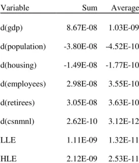
For reasonable confidence intervals (90%, 95% and 99%), the coefficients of the model retain their constant sign, which demonstrates the stability (robustness) of the estimate. Also, the minimum value of the sum of squares of the errors in the model (the gradient of the objective function is practically zero) is reached:
Table 4. The gradient of the objective function for the estimated parameters
Variable Sum Average
d(gdp) 8.67E-08 1.03E-09
d(population) -3.80E-08 -4.52E-10
d(housing) -1.49E-08 -1.77E-10
d(employees) 2.98E-08 3.55E-10
d(retirees) 3.05E-08 3.63E-10
d(csnmnl) 2.62E-10 3.12E-12
LLE 1.11E-09 1.32E-11
HLE 2.12E-09 2.53E-11
Source: authors processing, the table is obtained in EViews using the program sequence: View/Gradients and Derivatives/Gradient Summary.
function, which means that the objective function reached the optimal value. In the regression model, estimated by the least squares method, the objective function is calculated as the sum of the squares of the differences between the values of the endogenous variable (WEEE) and the model estimated values. The optimal value of the objective function implies that the sum should be minimal.
The estimated model is:
d(weeeit) = 0.042861·d(gdpit) + 0.023684·d(populationit) + 0.002145·d(housingit) +
+ 0.006251·(employeesit) + 0.854358·d(csnmnlit) – 0.055987·d(retireesit) +
+ 1.422585·LLEi – 2.098748·HLEi + d(εit) (8)
4. Conclusion
The size of the economic activity (approximated by GDP and number of employees) is positively associated with the collection of waste, as well as with income, population or the number of housings growth, which means that for an increase in the variables GDP, number of employees, salary, population, number of housings, the amount of WEEE collected also increases. The increase of the number of retirees and of the proportion of people with higher or average education is associated negatively with the collection of WEEE, i.e., if the number of retirees and of the proportion of population with higher or average education increases, the amount of WEEE collected decreases, and causes can be different: the relatively low income of retirees can generate a behaviour of preservation and storage for a long period of those objects and appliances, and the higher income of the educated population enables the purchase of more efficient appliances, with a longer life. Or, compared to the recorded incomes, the compensation for handing over old appliances is not appealing.
As a result of applying the model, we identified that independent variables such as population size, economic activity level (regional GDP and number of employees), income (monthly average net nominal earnings), various social groups such as county population (employed, unemployed , retired), existing housing, level of education and other non-quantifiable factors with regional influence considered invariants on the short-term (skills, beliefs, traditions, customs, etc.) affect the collection of WEEE only by 35%. This means that there are other factors influencing the collection of waste electrical and electronic equipment, such as: the development of a regional network of collection units, compensation attractiveness, visibility and effectiveness of campaigns to support those activities, etc.
References:
[1] ANPM, Informaţii privind gestionarea deşeurilor de echipamente electrice şi electronice, www.anpm.ro,
2015, accessed on 08/20/2015.
[2] Colesca, S.E., Ciocoiu, C.N. & Popescu, M.L., Determinants of WEEE Recycling Behaviour in Romania: A fuzzy Approach, International Journal of Environmental Research, Vol. 8, No. 2, 2014, pp. 353-366. [3] Cucchiella, F., D’Adamo, I., Koh, S.C. Lenny & Rosa, P., Recycling of WEEEs: An economic assessment
of present and future e-waste streams, Renewable and Sustainable Energy Reviews, Vol. 51, 2015, pp. 263–272, http://dx.doi.org/10.1016/j.rser.2015.06.010.
[4] Cucchiella, F., D’Adamo, I. & Gastaldi, M., Sustainable management of waste to energy facilities. Renew Sustain Energy Rev, Vol. 33, 2014, pp. 719–28.
[5] Eurostat, Waste Electrical and Electronic Equipment,
http://ec.europa.eu/eurostat/c/portal/layout?p_l_id=664648&p_v_l_s_g_id=0, accessed on 02/10/2015. [6] INS, Statistici privind populaţia României, http://statistici.insse.ro/, 2015, accessed on 07/17/2015.
[7] Jula D., Econometria datelor de tip panel, Academia Română – proiectul READ, 2014, p. 21-25, http://mone.acad.ro/wp-content/uploads/2014/09/Panel-Jula.zip.