5
EFFECTS OF TEMPORAL RESOLUTION ON RIVER FLOW
FORECASTING WITH SIMPLE INTERCEPTION MODEL WITHIN A
DISTRIBUTED HYDROLOGICAL MODEL
Azinoor Azida ABU BAKAR1 & Minjiao LU2,3
1Graduate Student, Dept. of Civil and Environmental Engineering,
Nagaoka University of Technology, Kamitomioka 1603-1, Nagaoka, Niigata, 940-2188 Japan. 2Dr. of Eng., Professor, Dept. of Civil and Environmental Engineering,
Nagaoka University of Technology, Kamitomioka 1603-1, Nagaoka, Niigata, 940-2188 Japan. 3Dr. of Eng., Adjunct Professor, School of River and Ocean Engineering,
Chongqing Jiaotong University, Chongqing, China
ABSTRACT
The effect of temporal resolution of hydrological data on the rainfall-runoff simulation is presented in this paper. The interception phenomenon is normally considered as one of the losses in hydrological cycle that comes into intention of many hydrologists for several decades. Distributed hydrological model developed by Lu et al, 1989 [1] with a simple interception model was implemented. The rainfall-runoff simulation is carried out at Doki River basin, Kagawa Prefecture, Japan. The river basin area is 106.8 km2 where most of the basin area is covered by the forest and the influences of human activities are very limited. Interception is considered as an important hydrological process in simulating the rainfall-runoff hydrograph for this basin. Rainfall data with a different temporal resolution ranging from one hour to twenty four hours are processed as the input and the model shows the different responses to each of the hydrological data with different temporal resolution.
Keywords : Distributed hydrological model, temporal resolution, interception
1. INTRODUCTION
Canopy interception is the phenomena where the water does not reach the ground. The capacity of the water to be intercepted and stored is now become an important study to many hydrologists. Canopy interception is considered as an important hydrological process in simulating the rainfall-runoff hydrograph for the basin since the losses by this phenomenon is about 25% of the rainfall depending on the nature of the rainfall and the size of the canopy storage capacity (Eltahir & Bras, 1992) [2]. Interception also plays an important role in partitioning the rainfall into evaporation and runoff (Baki, 1997) [3].
From the previous study (Rutter et al., 1971 [4]; Rutter and Morton, 1977 [5]; Gash and Morton, 1978 [6]; Gash, 1979 [7]), the researchers found that canopy structure, evaporation rate during storm and rainfall rate are the factors affecting the rate of interception loss, and Gash et al., 1979 [7] found that the evaporation of intercepted water is a major role in the water balance, especially during the long periods of gentle rain.
Liu et al. (2000) [8] mentioned that canopy interception is affected by vegetation, meteorological and rainfall factors. Meteorological factors can determine the water loss by evaporation process during the rainfall event. The rainfall is significantly distributed with time and space within the catchment area. Others study shows that the changed of time and spatial resolution of rainfall data can cause a significant effect to estimate the river discharge (Ishidaira et al., 2003) [9]. However, the effect of the temporal resolution to the distributed hydrological model with interception process is not yet clear. Therefore, the objective of this study is to investigate the effects of temporal resolution of hydrological data on the rainfall-runoff simulation. The rainfall-runoff simulation is carried out in the Doki River basin at Kagawa Prefecture, Japan. The hydrological model applied is a distributed one developed by Lu
6 2. METHODOLOGY
2.1 Basin characteristics
The basin area, named Doki River basin, is located in Kagawa Prefecture, Shikoku Island, western part of Japan. This is a small river basin just about 106.8 km2 where most of the basin area is covered by the forest and the influences of human activities are very limited. There are 7 types of landuse classes in the basin as shown in Table 1. Due to the geographical location, Doki river basin receives 1600 mm annual rainfall and the annual evaporation is 780 mm. For this case, snowmelt is considered not so significant because the upper part of the Doki river basin has no snow during the winter.
Table 1. Land cover in the Doki river basin (Makino et al., 1999) [10].
Landuse Land cover (%)
Forest 85.5
Paddy field 5.6
Vegetable field 6.2
Bare soils 1.1
Grass 0.2
Urban area 0.9
Water 0.5
2.2 Data preparation
Long series of rainfall data are taken as input to the model to simulate long time series of runoff. The rainfall data was calculated using a rainfall data set of 245 448 in the period between January 1978 and December 2005 (28 years). The data was collected from 16 stations from two sources. The AMeDAS rainfall data was provided by the Japan Meteorological Agency and the site data is collected by Ministry of Land, Infrastructure, Transport and Tourism Japan. It is based on the hourly data. The locations of the stations are listed in Table 2 and as shown in Figure 1.
Table 2. Locations and elevations of seven AMeDAS stations in Kagawa Prefecture, Japan.
Station Type of Data
Latitude (deg)
Longitude (deg)
Tadotsu AMeDAS 34.273 133.775
Takamatsu AMeDAS 34.313 134.057
Hiketa AMeDAS 34.210 134.410
Uchinomi AMeDAS 34.492 134.303 Takinomiya AMeDAS 34.235 133.928
Saita AMeDAS 34.117 133.775
Ryuozan AMeDAS 34.112 134.053
7
Figure 1. Location of AMeDAS and observed stations at Kagawa Prefecture, Japan.
To temporate the data, the hourly precipitation data was calculated as an average value for each resolution. In this process, the total precipitation during divisions is preserved for all temporal resolutions. For example, for time resolution 2 hours, the precipitation is divided into P1,1 and P1,2 in two subperiods. The time step of the subperiod is
fixed as one hour but the averaging time for every rainfall event is changed. This is to avoid the computational error during calculation. Figure 2 illustrates the temporal resolution applied to prepare the data.
Figure 2. The time step is fixed but the time of rainfall event is averaged.
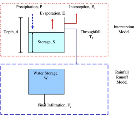
2.3 Interception model
Figure 3 shows the interception model and rainfall-runoff model applied in this study. Rainfall is the major input in this model. The basic Gash analytical concept (Gash, 1979) [7] works on bulk rainfall input, canopy structure parameters, and evaporation of intercepted water was applied to this model. There are several assumptions made to the concept. It was assumed that there is no water drips from the canopy before the canopy capacity is filled; the rainfall pattern is represented by a series of discrete storms which are separated by sufficiently long intervals to allow the canopy to dry; the rainfall and the evaporation rates are constants during the storm, and under the conditions of canopy saturation the mean rainfall and evaporation rates are used; and evaporation from stems occurs only when the rainfall has ceased.
1 2 3 4 5 6 7 8 Time
P
P1/2 P1
P1/3 P2
P2/2
8
Precipitation, P Interception, Ec
Depth, d
Storage, S
Throughfall, Tf
Water Storage, W
Interception Model
Rainfall Runoff
Model
Final Infiltration, Fc
Evaporation, E
Precipitation, P Interception, Ec
Depth, d
Storage, S
Throughfall, Tf
Water Storage, W
Interception Model
Rainfall Runoff
Model
Final Infiltration, Fc
Evaporation, E
Figure 3. Interception and runoff model.
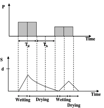
In basic description of the interception process, the rainfall event can be characterized by the rainfall intensity, storm duration, Td; and storm break period, Tb. During the rainfall event, there are three phases that the canopy water
storage undergoes that are wetting phase, saturation phase and drying phase but if the storm intensity is too weak or the duration of the rainfall is too short, the canopy does not reach the saturation before the storm ends. For this case, there are only two phases involve that are wetting and drying phase. This process is illustrated in Figure 4.
P
Time Td Tb
Time Wetting Drying
Saturation Wetting Drying S
d P
Time Td Tb
P
Time Td Tb
Time Wetting Drying
Saturation Wetting Drying S
d
Time Wetting Drying
Saturation Wetting Drying S
d
Time Wetting Drying
Saturation Wetting Drying S
9
P
T
dT
bTime
Time
Wetting
Drying
Wetting
Drying
S
d
P
T
dT
bTime
P
T
dT
bTime
Time
Wetting
Drying
Wetting
Drying
S
d
Figure 4. Basic description of interception concept and temporal resolution.
When the temporal resolution apply to the rainfall data, it effect the duration of the storm and the storm break period. The storm duration will be longer and shorten the break period. This may reduce the rainfall intensity.
The conditions considered to determine the interception are as follows:
S
d
P
S
d
P
S
d
P
T
f0
)
(
(1)
S
E
E
S
E
S
E
p p
p
c
(2)
where Tf is the throughfall, P is the rainfall, d is the depth of storage capacity, S is the storage, Ec is the interception
and Ep is the potential evaporation. The throughfall will occur when the rainfall is exceeding the storage capacity but
no throughfall is allowed when the canopy is unsaturated. This will affect occurrence of the interception values. For evaporation greater than storage capacity, the interception value is the storage capacity but if the evaporation is equivalent or lesser than the storage capacity, the interception is the evaporation value. For all cases, the throughfall is the new input rainfall data for the rainfall-runoff routing.
2.4 Distributed hydrological model
The distributed hydrological model used in this study is from the model developed by Lu et al., 1989 [1]. This model consists of three sections: routing, runoff and snowmelt analysis. For this study, the routing process applied is the kinetic wave method; rainfall-runoff model is Xinanjiang model but no snowmelt analysis because the basin did not receive snow during winter.
Xinanjiang rainfall-runoff model is a conceptual watershed model developed at Hihai University, China in 1970s. It provides an integral structure, statistically describing the non-uniform distribution of runoff producing areas, which features it as one of the conceptual, semi-distributed hydrological models developed. The model consists of 15 parameters, as shown in Table 3 and performs best for the humid and semi-humid catchments (Hapuarachchi, 2003) [11].
10
models are areal mean rainfall, and evaporation. Besides, the sub-catchment areas, and initial state of the catchment are necessary for the calculations. A complete description of Xinanjiang model can be found inZhao, 1992 [13].
The potential evaporation, Ep is calculated by Priestley-Taylor equation (Priestley and Taylor, 1972) [14] expressed
by Eq. (3)
n
p
R
E
(3)
where
is the Priestley-Taylor constant (1.26);
is the slope of saturation vapor pressure function of
temperature,
a satdT
de
;
is psychometric constant (0.677); and
R
nis the net radiation. But in this study, the
potential evaporation is calculated as Eq. (4).
p
p
E
E
'
0
.
4
(4)
Table 3. Parameters of the Xinanjiang model.
Parameters Description
Interception WUM Tension water capacity of upper layer WLM Tension water capacity of lower layer C Interception coefficient of deeper layer Runoff
Generation WM Areal mean tension water capacity B Exponential of the distribution of
tension water capacity
IM Ratio of impervious area to the total area of the basin
SM Free water storage capacity Runoff
Separation
EX Exponential of distribution water capacity
KG Outflow coefficient of free water storage to the ground water flow KI Outflow coefficient of free water
storage to the inter flow Runoff
Concentration
CG The recession constant of ground water storage
CI The recession constant of lower interflow storage
CS The recession constant of channel network storage
Flow Routing XE Muskingum coefficient
This value is already calibrated in the previous study (Yamamoto and Lu, 2008) [12]. Rn is calculated by Eq. (5).
inn
albedo
R
R
1
(5)
The slope of saturation vapor pressure function of temperature is determined by the saturation vapour pressure, esat
and temperature, Ta (Cel deg) of the ground. esat was calculated by Eq. (6).
8
.
242
6
.
4278
exp
10
749
.
2
8a sat
T
x
11 2.5 Statistical indices
By using the simulated discharge calculated by the model and the observed discharge obtained from the site, the model performance was evaluated by using the Nash efficiency coefficient. The difference between the observed and simulated discharge is evaluated by Eq. (7):
n
i
obs obs n
i
calc obs
f
Q
Q
Q
Q
E
1
2 1
2
1
(7)where Qcalc is the simulated discharge, Qobs is the observed discharge, and
Q
obsis the mean observed discharge.Nash efficiency coefficient is the proportion of the variance of the observed values accounted by the model. The value can be ranged from minus infinity to one. A negative value indicates that the observed mean does better prediction of the observed value than the model. A higher value indicates good agreement between the observed with the calculated hydrograph
3. RESULTS AND DISCUSSIONS
This study focuses on the effects of temporal resolution of river flow forecasting with interception model implemented to the distributed hydrological modeling. As results, the changes of hydrograph produced with the different temporal resolution are determined. The difference between the hydrographs of each simulation is evaluated through the Nash efficiency, Ef. The ratio of the interception loss to the evaporation and the ratio of
interception to total rainfall are also established.
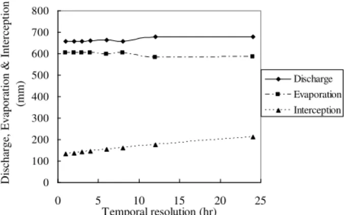
Figure 5 and Figure 6 show the value of the mean discharge, evaporation and interception for each temporal resolution, and the ratio of interception to rainfall and total evaporation for each temporal resolution, respectively. Results from Figure 5 shows that the temporal resolution is proportional to the product of discharge and interception but disproportional with evaporation. It is also found that interception loss increased with rainfall intensity when the rainfall duration lasted equally long. This is because some part of the precipitation is stored in the canopy. As long as the canopy is unsaturated, a high fraction of rain can be intercepted. When the canopy is saturated, most of the rain that falls on the vegetation will drain to the ground and interception can only increase by evaporation during rain.
0 100 200 300 400 500 600 700 800
0 5 10 15 20 25
Temporal resolution (hr)
Discharg
e,
Evap
orati
on
&
Interce
ptio
n
(mm)
Discharge Evaporation Interception
12
0 5 10 15 20 25 30 35 40
1 2 3 4 6 8 12 24
Temporal resolution (hr)
E
c
/P
, E
c
/E
(%) Ec/P
Ec/E
Figure 6. Proportions of interception with precipitation and evaporation.
The fraction of intercepted with rainfall and evaporation is not only rather large, but also variable in time. In particular, a higher fraction is intercepted from small rain events which mean the interception loss fraction is high at temporal resolution 24 hours compared to temporal resolution 1 hour. Therefore for a different rainfall event but with the same total rainfall amount, the heavy rainfall may produce less interception loss compare to the light rainfall.
The dissimilarity between the observed and simulated discharge for each temporal resolution is shown in Figure 7. The figure shows the hydrograph for year 2005. It can be seen that the temporal resolution cause significant effect to the hydrological simulation where the temporal resolution factor reduce the peak discharge of the simulated hydrograph. This is because when the temporal resolution apply to the rainfall data, it effect the duration of the storm and the storm break period. The soil is kept in wet condition for a long time due to the longer precipitation duration. This will increase the potential evaporation from the land surface.
In order to evaluate the model, the discharge simulated by the model is compared with the observed discharge by using Nash efficiency score.
0 50 100 150 200 250 300
0 2 4 6 8 10 12 14
Month, 2005
D
is
cha
rg
e
TR=1 TR=2 TR=4 TR=12 TR=24 Obs
Figure 4. Observed and simulated discharge for each temporal resolution.
Table 4. Nash efficiency value for each temporal resolution.
Temporal Resolution (hr)
Nash Efficiency, Ef
1 0.655
2 0.657
3 0.654
4 0.651
6 0.641
8 0.621
12 0.582
24 0.462
13
hydrograph. It can be seen that the higher the temporal resolution, the lower the Nash efficiency values which mean poor agreement between the observed and the calculated hydrograph. In this study the hydrograph is simulated for a long period of time that is 28 years (1978-2005). The effect of the wet condition may not affect the simulated hydrograph.
4. CONCLUSION
From this study, the influence of temporal resolution to the simulated hydrograph is determined. The result shows that the temporal resolution is significantly effected the production of simulated hydrograph. For each resolution, the difference between the hydrographs of each temporal resolution is evaluated through the Nash efficiency value and the results show that the lower the temporal resolution, the more simulated hydrographs agree with the observed discharge in terms of the variance.
5. REFERENCES
[1]. Lu, M., Koike, T., & Hayakawa, N.: A model using distributed data of radar rain and altitude. Proc. JSCE, 411/11-12, 135-142, 1989.
[2]. Eltahir, E. A. B. & Bras, R. L.: A description of rainfall interception over large areas. Journal of Climate. Vol 6, 1002-1008, 1992.
[3]. Baki, A.: Hydrological processes in land phase hydrology. Journal of the Institution of Engineers Malaysia, Vol. 58, No. 1, 11-21 (1997).
[4]. Rutter, A.J., Kershaw, K.A., Robins, P.C., Morton, A.J.: A predictive model of rainfall interception in forests. I-Derivation of the model from observations in a plantation of Corsican pine. Agric. Meteorol., 9, 367-384, 1971.
[5]. Rutter, A.J., Morton, A.J.: A predictive model of rainfall interception in forests. III - Sensitivity of the model to stand parameters and meteorological variables. J. Appl. Ecol., 14.567-588, 1977.
[6]. Gash, J.H.C., Morton, A.J.: An application of the Rutter mode1 to the estimation of the interception loss from the Thetford forest. J. Hydrol., 38.49-58, 1978.
[7]. Gash, J. H. C.: An analytical model of rainfall interception by forests. Quart. J. R. Met. Soc, 105, 43-55, 1979.
[8]. Liu, J. G., Wan, G. L., Zhang, X. P., Wang, B. N.: Semi-theoretical model of rainfall interception of forest canopy. Seientia Silvae Sinicae 36, 2-5, 2000.
[9]. Ishidaira, I., Takeuchi, K., Xu, Z., Ao, T., Magome, J. & Kudo, M.: Effect of spatial and temporal resolution of rainfall data on the accuracy of long-term runoff simulation. Weather Radar Information and Distributed Hydrological Modelling. IAHS Publ. no 282, 2003.
[10]. Makino, I., Ogawa, S. and Saito, G.: Land cover change and its effect on runoff in the Doki river catchment.
Proceedings of 20th Asian Conference on Remote Sensing, 1999.
[11]. Hapuarachchi, H. A. P., Li, Z. and Wolfgang, F. A.: Application of the SWAT model for river flow forecasting in Sri Lanka. Jour. Of Lake Sciences, Vol. 15, 2003.
[12]. Zhao, R. J.: The Xinanjiang model applied in China. Journal of Hydrology, 135 (1992) 371-381, 1992. [13]. Priestley, C.H.B. and Taylor, R. J.: On the assessment of surface heat and evaporation using large-scale
parameters. Mon. Weather Rev. 100, 81-92, 1972.
[14]. Yamamoto, T. and Lu, M.: Long term distributed rainfall runoff analysis and its application to river planning,
![Table 1. Land cover in the Doki river basin (Makino et al., 1999) [10].](https://thumb-eu.123doks.com/thumbv2/123dok_br/18346954.352619/2.918.340.584.347.513/table-land-cover-doki-river-basin-makino-et.webp)