Introducing upfront losses as well as gains decreases impatience in intertemporal choices with rewards

(1)

Introducing upfront losses as well as gains decreases impatience in

intertemporal choices with rewards

Cheng-Ming Jiang

∗

Feng-Pei Hu

†

Long-Fei Zhu

†

Abstract

People tend to prefer smaller and sooner (SS) rewards over larger and later (LL) ones even when the latter are much larger. Previous research have identified several ways to enhance people’s patience. Adding to this literature, the current paper demonstrates that introduction of upfront losses as well as gains to both SS and LL rewards can decrease people’s impatience. This effect is incompatible with both the normative exponential and descriptive hyperbolic discounting mod-els, which agree on the additive assumption and the independence assumption. We also exculde the integration explanation which assumes subjects integrate upfront money with final rewards and make a decision with bottom line at the end. We consider several possible explanations, including the salience hypothesis, which states that introducing upfront money makes the money dimension more salient than not and thus increases the attractiveness of LL options.

Keywords: intertemporal choice, impatience, upfront losses, upfront gains.

1 Introduction

Intertemporal choices, or decisions whose outcomes are determined over time, such as choosing between saving money for education and spending it on a luxury item, are ubiquitous and important in everyday life. The disposition to choose a larger, later reward over a tempting, sooner one and the tendency to focus on the future relate to impor-tant individual outcomes, such as academic achievement (Duckworth & Seligman, 2005). Sooner rewards are usu-ally difficult to resist. Excessive discounting can disrupt the achievement of long-term goals.

To study intertemporal choices, researchers (e.g., Estle, Green, Myerson, & Holt, 2007) have typically instructed subjects in their studies to choose between smaller and sooner (SS) rewards and larger and later (LL) ones (e.g., gaining CNY 210 in a week versus gaining CNY 250 in five weeks in the present study). People generally tend

This research was partially supported by the Zhejiang Provin-cial Philosophy and SoProvin-cial Science Planning Project of China (No. 14NDJC172YB), the Zhejiang Provincial Natural Science Foundation of China (No. LY14C090002), and the National Social Science Foundation of China (No. 14BSH070). The authors would like thank the two anony-mous referees and Editor Jonathan Baron for their valuable comments and suggestions on the draft of this paper. The authors also wish to thank Ren Yanju, Zhen Shiliang, Dong Huahua, and Kong Lin for collecting the data used in this study.

∗_{Center for Brain and Management Science, College of Economics}

and Management, Zhejiang University of Technology, 288 Liuhe Road, Xihu District, Hangzhou (310023), P.R.China. E-mail: jiangcheng-ming@zjut.edu.cn.

†_{Center for Brain and Management Science, College of Economics}

and Management, Zhejiang University of Technology.

to be impatient in such situations, and most prefer SS re-wards over LL rere-wards (even with a yearly interest rate of 965% in the above example).

Researchers have identified several ways to enhance people’s patience. For example, Urminsky and Kivetz (2011) demonstrated that adding an immediate token ward to both options increases the preference for LL re-wards. Magen, Dweck, and Gross (2008) showed that ex-plicitly referring to the hidden zero in each option (e.g., gaining CNY 210 in a week and CNY 0 in five weeks ver-sus gaining CNY 250 in five weeks and CNY 0 in a week) would decrease the willingness of subjects to choose im-mediate rewards. Read, Frederick, Orsel, and Rahman (2005) found that framing delays (e.g., in a period of six months) in corresponding calendars (e.g., on October 17) promotes the attractiveness of LL rewards.

The present paper introduces a novel way to decrease people’s impatience. The hypothesis is that adding upfront losses as well as gains, even small ones, to both options (i.e., SS and LL rewards) can enhance people’s patience and encourage them to choose LL options. The hypothesis is built on the assumption that introducing losses as well as gains may make the money dimension more salient and thus increase the attractiveness of LL options.

Experiment 1 shows that introducing upfront losses to both intertemporal options (i.e., SS and LL rewards) re-duces people’s impatience in both between- and within-subject designs and excludes the normative exponential and descriptive hyperbolic discounting models, which share assumptions of additivity and independence. Ex-periment 2 excludes an integration explanation, which as-sumes subjects integrate upfront money with final rewards

(2)

Table 1: Questionnaire items and summary of the results for Experiments 1A and 1B. (Φis effect size.)

Item (proportion of responses, %)

Experiment Pure gain Mixed condition p(Φ)

1A (same losses are added to SS and LL in the mixed condition)

Gain 120 yuan in a week (87.5) vs. Gain 150 yuan in 4 weeks (12.5)

Lose 100 yuan now and gain 120 yuan in a week (70.5) vs. Lose 100 yuan now and gain 150 yuan in 4 weeks (29.5)

0.004 (0.21)

Lose 11 yuan now and gain 210 yuan in a week (70.5) vs. Lose 11 yuan now and gain 250 yuan in 5 weeks (29.5)

0.004 (0.21)

Gain 3500 yuan in a year (71.2) vs. Gain 5800 yuan in 3 years (28.8)

Lose 160 yuan now and gain 3500 yuan in a year (55.2) vs. Lose 160 yuan now and gain 5800 yuan in 3 years (44.8)

0.022 (0.16)

< .001 (0.29)

1B (different losses are added to SS and LL in the mixed condition)

Lose 100 yuan now and gain 120 yuan in a week (46.2) vs. Lose 105 yuan now and gain 150 yuan in four weeks (53.8)

< .001 (0.43)

Lose 11 yuan now and gain 210 yuan in a week (55.7) vs. Lose 16 yuan now and gain 250 yuan in four weeks (44.3)

0.002 (0.32)

< .001 (0.39)

< .001 (0.41)

and make a decision with bottom line at the end. The ex-periment also corroborates the previous reported upfront gain effect (Urminsky & Kivetz, 2011): adding upfront gains (rather than losses) to both SS and LL options can also enhance people’s patience. In the general discussion, we consider the possible causes for this upfront loss as well as gain effect.

2 Experiment 1

2.1 Method

In Experiment 1A, 209 undergraduates (55 males, Mage= 21.3, SD = 1.4) from Shangdong Normal University and Shanghai Second Polytechnic University attended in a class. Each of the subjects was randomly assigned to one of two conditions. Subjects in the pure gain condition re-sponded to typical choice pairs (e.g., gaining CNY 210 in a week versus gaining CNY 250 in five weeks), whereas those in the mixed condition had the same choices except that both options begin with a same immediate loss (e.g., losing CNY 11 now and gaining CNY 210 in one week versus losing CNY 11 now and gaining CNY 250 in four weeks).

To ask whether the results hold for different rewards as well as for different upfront losses, we varied the

re-wards (from CNY 100 to CNY 8,000) and the upfront losses (from 5% to 89% of some sooner rewards) over a wide range. The subjects indicated their preferences in the questionnaire, which consisted of four pairwise choices and was presented on paper (Table 1).

The pure gain condition in Experiment 1B is the same as that in Experiment 1A. In the mixed condition, different upfront losses were introduced into the SS and LL options. That is, the losses in the LL option are always CNY 5 more than those in the SS options (e.g., losing CNY 11 now and gaining CNY 210 in a week versus losing CNY 16 now and gaining CNY 250 in five weeks) (Table 1).

(3)

2.2 Results and discussion

Consistent with the hypothesis, both Experiments 1A and 1B demonstrate that the introduction of upfront losses to both intertemporal options (i.e., SS and LL) reduces people’s impatience regardless of whether the immediate losses are small or large. Table 1 summarizes the results. These results are directly inconsistent with the established models of intertemporal choice. Both the (normative) exponential model (i.e., discounted-utility, Samuelson, 1937) and (descriptive) hyperbolic discounting models (e.g, hyperbolic discounting model, Mazur, 1984; quasi-hyperbolic discounting model, Laibson, 1997) generally agree on the additivity assumption and the independence assumption when these models are applied to intertempo-ral choice between pairs of multiple-dated outcomes (Rao & Li, 2011). The additivity assumption means that pref-erences for multiple-dated outcomes are based on a sim-ple aggregation of their individual components within in-tertemporal options (Loewenstein & Prelec, 1993) and the independence assumption means that the utility of an out-come in one period is independent of outout-comes in other periods (Prelec & Loewenstein, 1991). This implies that the relative evaluations of the options in the pure gain and mixed conditions are equivalent in Experiment 1A and should be biased towards SS options in the mixed condi-tions of Experiment 1B. In Experiment 1A, if people pre-fer SS options over LL ones in the pure gain condition, they should also prefer the same options in the mixed con-dition because the common elements of loss should not change their preference. In Experiment 1B, in which the upfront losses in the SS options are always less than those in the LL ones in the mixed condition, if people prefer SS options over LL ones in the pure gain condition, they will also prefer the corresponding SS options in the mixed con-dition. However, the preferences in Experiment 1A and 1B were both changed in favor of LL in the mixed conditions. Thus, the exponential discounting model and hyperbolic discounting models, both of which assume additivity and independence, cannot account for this upfront loss effect.

Now we consider whether or not the integration hypoth-esis (Thaler, 1985), which does not assume additivity and independence, can account for the observed effect. This hypothesis posits that, when people face problems such as choosing between “losing CNY 100 now and gaining CNY 120 in a week” and “losing CNY 100 now and gain-ing CNY 150 in 4 week,” they need to think only about the bottom line at the end and subtract the initial loss from the final reward, which is “CNY 20 in a week” versus “CNY 50 in four weeks” in this example. This process increases the ratio of outcomes of LL options to those of SS options and may encourage the subjects to choose the LL options. Therefore, in the next experiment, we check whether the integration hypothesis can account for this effect.

3 Experiment 2

3.1 Experiment 2A

We assumed that, if the integration hypothesis is correct, people will integrate an initial reward — if the initial out-come is a reward instead of a loss (e.g., gain CNY 100 now and gain CNY 120 in a week) — with the final re-ward in a mixed intertemporal choice option. In Experi-ment 2A, we used pairwise options that begin with a con-stant gain, rather than a loss, to examine the integration hypothesis. It can be assumed that the difference in de-lay between SS and LL options has the effect of multi-plying u(MSS) by a constant K that is greater than 1,

where MSS is the amount of money received in the SS

option andu(MSS)is its utility. Thus, a LL option will

be chosen if u(MLL)/u(MSS) > K, a SS option will

be chosen ifu(MLL)/u(MSS) < K, and a subject will

be indifferent ifu(MLL)/u(MSS) = K, whereMLL is

the amount of money received and u(MLL) is its

util-ity in a LL option. Now we consider that an amount

C > 0 is added to bothMLL andMSS. Most studies

on intertemporal choice assumed linear utility and some assumed concave utility for gains and convex utility for losses (e.g., Loewenstein & Prelec, 1992). A few empiri-cal studies have confirmed the latter (Abdellaoui, Attema, & Bleichrodt, 2009). Thus, we can assume linear utility or concave utility for gains here. SinceC >0andMLL >

MSS,u(MLL+C)/u(MSS+C)< u(MLL)/u(MSS).

This implies that, ifu(MLL)/u(MSS) < K,u(MLL+

C)/u(MSS+C)< Kaccording to the transitivity rule.1

In sum, if subjects prefer SS over LL options in the pure condition, and if the integration hypothesis is correct, they should also prefer SS over LL options in the mixed condi-tion in which pairwise opcondi-tions begin with a same immedi-ate gain. This inference can also be extended to the situ-ation in which immediate reward has greater impact than final reward, because we only need to adjust the impact of C by a weight greater than 1.

3.1.1 Method

In Experiment 2A, 171 students (82 males, Mage= 20.8, SD = 1.5) from Zhejiang University of Technology were approached in the library and randomly assigned to either one of two conditions: In the pure gain condition, the sub-jects responded to typical choice pairs as in Experiment 1A (e.g., gaining CNY 210 in a week versus gaining CNY 250 in five weeks), whereas those in the mixed condition responded to choice pairs beginning with the same upfront rewards (e.g., gaining CNY 11 now and gaining CNY 210 in a week versus gaining CNY 11 now and gaining CNY

1_{Thanks to Editor Jonathan Baron for helping us to clarify this}

(4)

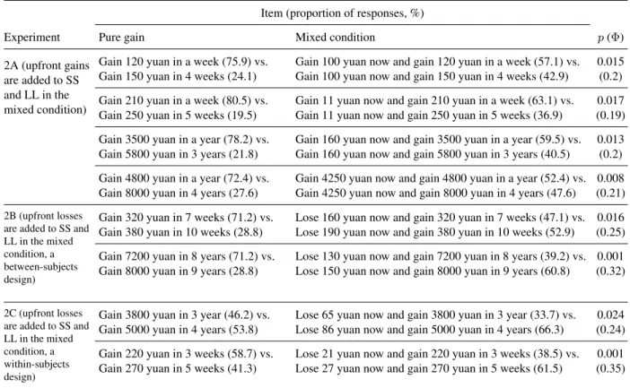
Table 2: Questionnaire items and summary of the results for Experiments 2A, 2B, and 2C. (Φis effect size.)

Item (proportion of responses, %)

Experiment Pure gain Mixed condition p(Φ)

2A (upfront gains are added to SS and LL in the mixed condition)

Gain 100 yuan now and gain 120 yuan in a week (57.1) vs. Gain 100 yuan now and gain 150 yuan in 4 weeks (42.9)

0.015 (0.2)

Gain 11 yuan now and gain 210 yuan in a week (63.1) vs. Gain 11 yuan now and gain 250 yuan in 5 weeks (36.9)

0.017 (0.19)

Gain 160 yuan now and gain 3500 yuan in a year (59.5) vs. Gain 160 yuan now and gain 5800 yuan in 3 years (40.5)

0.013 (0.2)

Gain 4250 yuan now and gain 4800 yuan in a year (52.4) vs. Gain 4250 yuan now and gain 8000 yuan in 4 years (47.6)

0.008 (0.21)

2B (upfront losses are added to SS and LL in the mixed condition, a between-subjects design)

Gain 320 yuan in 7 weeks (71.2) vs. Gain 380 yuan in 10 weeks (28.8)

Lose 160 yuan now and gain 320 yuan in 7 weeks (47.1) vs. Lose 190 yuan now and gain 380 yuan in 10 weeks (52.9)

0.016 (0.25)

Gain 7200 yuan in 8 years (71.2) vs. Gain 8000 yuan in 9 years (28.8)

Lose 130 yuan now and gain 7200 yuan in 8 years (39.2) vs. Lose 150 yuan now and gain 8000 yuan in 9 years (60.8)

0.001 (0.32)

2C (upfront losses are added to SS and LL in the mixed condition, a within-subjects design)

Gain 3800 yuan in 3 year (46.2) vs. Gain 5000 yuan in 4 years (53.8)

Lose 65 yuan now and gain 3800 yuan in 3 year (33.7) vs. Lose 86 yuan now and gain 5000 yuan in 4 years (66.3)

0.024 (0.24)

Gain 220 yuan in 3 weeks (58.7) vs. Gain 270 yuan in 5 weeks (41.3)

Lose 21 yuan now and gain 220 yuan in 3 weeks (38.5) vs. Lose 27 yuan now and gain 270 yuan in 5 weeks (61.5)

0.001 (0.35)

250 in four weeks) (Table 2). Choice pairs was presented on paper. The subjects were given a small gift for their cooperation.

3.1.2 Results and discussion

The results demonstrate that the introduction of upfront rewards to both intertemporal options (i.e., SS and LL) re-duces impatience. Table 2 summarizes the results. These results are consistent with those of Urminsky and Kivetz (2011), although the time of the upfront gains (i.e., now) recieved in this study is a little differred from theirs (i.e., 1 day or 3 days delayed). These results however, are in opposition to the prediction of the integration hypothesis.

Although the results of Experiment 2A help to rule out the integration explanation, the subjects may possibly in-tegrate the upfront losses but not the upfront rewards with the final rewards in the mixed conditions. In Experiments 2B and 2C, we directly exclude the integration hypothesis.

3.2 Experiments 2B and 2C

We introduced larger losses to the LL options than to the SS options so that the ratio of the introduced losses in the LL options to those in the SS options would be equal to or a little larger than the ratio of rewards in LL options to

those in the SS options (Table 2). We assume that, if the subjects subtract the initial losses from the final rewards as hypothesized by the integration hypothesis, this inte-gration will not change or even decrease the ratio of the integrated amounts of the LL options to those of the SS options in the mixed condition, compared with the ratio of rewards of the LL options to those of the SS options in the pure condition. Therefore, the preference of sub-jects should change in favor of, or at least not in the op-posite direction of, the SS options based on the magnitude effect found in previous studies (Chapman & Winquist, 1998; Loewenstein & Prelec, 1992; Prelec & Loewen-stein, 1991). That is, by the integration hypthesis, deci-sion makers should show a large temporal discount rate for small magnitudes than for large ones.

Experiments 2B and 2C used between- and within-subjects designs, respectively, with choice options pre-sented to the subjects with little variation.

3.2.1 Method

(5)

and was given on paper. Five students did not respond in one or both pairwise choices and were therefore excluded. A total of 103 students remained (40males, Mage= 21.5, SD = 1.7) for the analysis.

Experiment 2C used a within-subjects design, in which each subject responded to each condition. Another 104 students (61males, Mage= 21.1, SD = 1.9) from Zhejiang University of Technology were approached in the library and asked to respond to the questionnaire consisting of four pairwise choices (with each condition having two pairs of choices) and other unrelated questions, which was given on paper. The order of the two conditions was coun-terbalanced. Thus, half of the subjects first answered the questions of the mixed condition followed by those of the pure gain condition, and the other half answered in the re-verse order.

All the subjects were presented with a small gift for their participation.

3.2.2 Results and discussion

The results of both Experiments 2B and 2C demonstrate that the introduction of upfront losses to both intertempo-ral options (i.e., SS and LL) made the subjects more prone to choose the LL options rather than the SS options, con-trary to the prediction of the integration hypothesis. Table 2 summarizes the results. Therefore, we can conclude that the integration explanation cannot account for the upfront loss effect.

4 General discussion

This paper shows that introducing upfront losses as well as gains decreases people’s impatience in intertemporal choices. In particular, the upfront loss effect has never been reported before. We also excludes the (normative) exponential model and (descriptive) hyperbolic discount-ing model, as well as the integration hypothesis, as an ac-count of these effects.

Although the aim of this paper is primarily to docu-ment the effect of upfront money, particularly, of upfront losses, we consider several other possible explanations for this effect. The first explanation is the salience hypoth-esis, which states that introducing losses as well as gains makes the money dimension more salient than not and thus increase the attractiveness of LL options. This account is comprehensive because it can account for all the results of the current study. Moreover, this hypothesis may explain the hidden zero effect and the mere token effect (Magen, Dweck, & Gross, 2008; Urminsky & Kivetz, 2011): The explicating of hidden-zero and the offering of a small to-ken reward may make the money dimension more salient

and thus increase the attractiveness of LL options.2 The second explanation is the time scale hypothesis, which assumes that the presentation of the 0-delay amount anchors the time dimension at 0.3 _{Thus, in the pure} con-dition, subjects maybe compare the delays beween SS and LL options and consider the delay of LL option with the reference point at the delay of SS option. For example, when facing a choice between “gaining CNY 320 in 7 weeks and gaining CNY 380 in 10 weeks”, the subjects might put the reference point at 7 weeks and think the de-lay of the LL reward is 3 weeks. In the mixed conditions, the subjects are more likely to look at the time ratios rather than their differences and thus feel the delays beween SS and LL options are much shorter than in the pure cond-tions. Therefore, they are more likely to choose LL op-tions in the mixed condiop-tions than in the pure condiop-tions.

The third explanation is the decision mode hypothe-sis, which posits that upfront losses may prompt people to adopt different modes of cognitive processing. In the pure gain condition, the subjects may respond with an au-tomatic cognitive mode, whereas in the mixed conditions, they may respond with a deliberate cognitive mode (Dune-gan, 1993), therefore increasing the attractiveness of the LL options over the SS ones in the latter situation. This explantion, however, is confined to the effect of upfront loss and can not account for the general effect of upfront money. Further research is required to elucidate the un-derlying mechanism of the effects reported here.

We used intervals no shorter than a week to study im-patience. Although they are consistent with some research (e.g., Urminsky & Kivetz, 2011), we should point out that most studies on impatience in intertempral choice used very short intervals, such as immediacy (e.g., Magen et al., 2008). Further research need to consider very short intervals.

Another limitation of the current study is that we used hypothetical rather than real money as outcomes, because

2_{Magen et al.(2008) speculated that the preference for sequences that}

improve over time or the attention to the opportunity cost of each choice induced by the explicit-zero format may account for the hidden zero ef-fect. The improve-over-time explanation of Magen et al. (2008) posits that people compare later rewards with earlier losses or gains. This com-parison may increase the attractiveness of LL options in our study. This explanation, in some degree, is similar to (and perhaps can be incorpo-rated into) the salience hypothesis, which states that people focus more on the money dimension when the upfront amounts are introduced. The opportunity-cost explanation of Magen et al. (2008) is that explication of zero may reminds people that future (immediate) rewards are the oppor-tunity costs of immediate (future) rewards. This cannot account for the reported effects here. Urminsky and Kivetz (2011) argued that offering a small token reward reduced peoples’ choice conflict between their de-sire for an immediate reward and a higher payoff available by waiting, making them easier to ignore the temptation of immediacy and hold out for LL rewards. This explanation cannot account for the effect of upfront losses, because adding an upfront loss would be expected to increase peoples’ desire for an immediate reward.

3_{Thanks Editor Jonathan Baron for putting forward this explanation,}

(6)

executing real losses (e.g., CNY 4250) with the subjects was impossible. Although several previous studies have shown that hypothetical financial intertemporal choice outcomes yield the same results as real outcomes (Bickel, Pitcock, Yi, & Angtuaco, 2009; Johnson & Bickel, 2002; Madden et al., 2004), additional research is required to test the effect reported in this study with real money in real-world settings. However, if further confirmed, this ef-fect has practical implications for policy makers and man-agers, specifically in encouraging citizens or employees to choose LL rewards instead of SS ones by letting them incur some losses first, even small ones.

References

Abdellaoui, M., Attema, A. E., & Bleichrodt, H. (2009). Intertemporal tradeoffs for gains and losses: An experi-mental measurement of discounted utility.he Economic Journal, 120(545), 845–866.

Bickel, W. K., Pitcock, J. A., Yi, R., & Angtuaco, E. J. C. (2009). Congruence of bold response across intertem-poral choice conditions: Fictive and real money gains and losses.The Journal of Neuroscience, 29(27), 8839– 8846.

Chapman, G. B., & Winquist, J. R. (1998). The magni-tude effect: Temporal discount rates and restaurant tips. Psychonomic Bulletin & Review, 5(1), 119–123. Duckworth, A. L., & Seligman, M. E. (2005).

Self-discipline outdoes IQ in predicting academic perfor-mance of adolescents. Psychological Science, 16(12), 939–944.

Dunegan, K. J. (1993). Framing, cognitive modes, and image theory: Toward an understanding of a glass half full.Journal of Applied Psychology, 78(3), 491–503. Estle, S. J., Green, L., Myerson, J., & Holt, D. D. (2007).

Discounting of monetary and directly consumable re-wards.Psychological Science, 18(1), 58–63.

Johnson, M. W., & Bickel, W. K. (2002). Within-subject comparison of real and hypothetical money rewards in delay discounting. Journal of the Experimental Analy-sis of Behavior, 77(2), 129–146.

Laibson, D. (1997). Golden eggs and hyperbolic discount-ing.The Quarterly Journal of Economics, 112(2), 443– 478.

Loewenstein, G. F., & Prelec, D. (1992). Anomalies in intertemporal choice: Evidence and an interpretation. The Quarterly Journal of Economics, 107(2), 573–597. Loewenstein, G. F., & Prelec, D. (1993). Preferences for sequences of outcomes. Psychological Review, 100(1), 91–108.

Madden, G. J., Raiff, B. R., Lagorio, C. H., Begotka, A. M., Mueller, A. M., Hehli, D. J., & Wegener, A. A. (2004). Delay discounting of potentially real and hypo-thetical rewards: II. Between-and within-subject com-parisons.Experimental and Clinical Psychopharmacol-ogy, 12(4), 251–261.

Magen, E., Dweck, C. S., & Gross, J. J. (2008). The hidden-zero effect: Representing a single choice as an extended sequence reduces impulsive choice. Psycho-logical Science, 19(7), 648–649.

Mazur, J. E. (1984). Tests of an equivalence rule for fixed and variable delays. Journal of Experimental Psychol-ogy: Animal Behavior Processes, 10, 426–436. Prelec, D., & Loewenstein, G. F. (1991). Decision making

over time and uncertainty: A common approach. Man-agement Science, 37(7), 770–786.

Rao, L. L., & Li, S. (2011). New paradoxes in intertempo-ral choice. Judgment and Decision Making, 6(2), 122– 129.

Read, D., Frederick, S., Orsel, B., & Rahman, J. (2005). Four score and seven years from now: The date/delay effect in temporal discounting. Management Science, 51(9), 1326–1335.

Samuelson, P. A. (1937). A note on measurement of util-ity.The Review of Economic Studies, 4(2), 155–161. Scholten, M., & Read, D. (2010). The psychology of

in-tertemporal tradeoffs. Psychological Review, 117(3), 925–944.

Thaler, R. (1985). Mental accounting and consumer choice.Marketing Science, 4(3), 199–214.