BLIND SOURCE SEPARATION AND IDENTIFICATION OF NONLINEAR MULTIUSER
CHANNELS USING SECOND ORDER STATISTICS AND MODULATION CODES
Carlos Alexandre R. FERNANDES
∗, G´erard FAVIER
I3S Laboratory
CNRS - University of Nice-Sophia Antipolis
2000 route des Lucioles, BP 121,
06903, Sophia-Antipolis Cedex, France.
[email protected] and [email protected]
Jo˜ao Cesar M. MOTA
GTEL Laboratory
Federal University of Cear´a
Campus do Pici, 60.755-640,
6007 Fortaleza, Brazil.
[email protected]
ABSTRACT
In this paper, a Blind Source Separation (BSS) and channel iden-tification method using second order statistics is proposed for non-linear multiuser communication channels. It is based on the joint diagonalization of a set of covariance matrices. Modulation codes (constrained codes) are used to ensure the orthogonality of nonlinear combinations of the transmitted signals, allowing the application of a joint diagonalization based estimation algorithm. This constitutes a new application of modulation codes, used to introduce temporal redundancy and to ensure some statistical constraints. Identifiability conditions for the problem under consideration are addressed and some simulation results illustrate the performance of the proposed method.
1. INTRODUCTION
This work deals with the Blind Source Separation (BSS) and sys-tem identification problem for nonlinear multiuser communication channels. The considered channel is modelled as a complex-valued linear-cubic Multiple-Input-Multiple-Output (MIMO) Volterra fil-ter, which consists of a generical representation of instantaneous linear-cubic polynomial mixtures. This kind of nonlinear models has important applications in the field of telecommunications to model wireless communication links with nonlinear power amplifiers [1] and uplink channels in Radio Over Fiber (ROF) multiuser commu-nication systems [2]. The ROF links have found a new important ap-plication with their introduction in microcellular wireless networks [3, 4]. This kind of network architecture provides to the system a better capacity, coverage and power consumption. Thus, it can also improve the system reliability and Quality of Service. The uplink transmission of such systems is done from a mobile station towards a Radio Access Point, where the transmitted signals are converted in optical frequencies by a laser diode and then retransmitted through optical fibers. Important nonlinear distortions are introduced by the electrical-optical (E/O) conversion [3, 4]. When the length of the optical fiber is short (few kilometers) and the radio frequency has an order of GHz, the dispersion of the fiber is negligible [5]. In this case, the nonlinear distortion arising from the E/O conversion pro-cess becomes preponderant [3, 4, 5]. Up to several Mbps, the ROF channel can be considered as a memoryless link [2, 3]. Thus, in a multiuser system, the wireless link can be viewed as a linear mix-ture and the overall uplink channel as a memoryless MIMO Wiener
∗Thanks to CAPES/Brazil agency for funding.
system [2], which is a particular case of the model considered in this work. Moreover, in this application, the channel nonlinearity is modelled as a third order polynomial [2, 3].
In what concerns the BSS problem for nonlinear systems, there are many works dealing with Post Nonlinear (PNL) mixtures [1, 6, 7]. Some nonlinear BSS techniques are performed in sev-eral steps (multi-stage processing) [1, 7] and some works use a joint diagonalization of spatio-temporal covariance matrices to perform some of these stages [1, 8]. However, in the context of communica-tion systems, the transmitted signals are often assumed to be white, which requires the use of some coding, like those developed in this paper, to introduce time correlation in the signals. There are few works dealing with the problem of BSS or/and identification of non-linear systems in the context of multiuser communication channels. Among them, we cite [9] that proposes a blind zero forcing based equalization technique for Code Division Multiple Access (CDMA) systems.
The technique proposed in this paper exploits the use of Sec-ond Order Statistics (SOS) of the received signals. Modulation codes (constrained codes) [10] are used to ensure the orthogonal-ity of nonlinear combinations of the transmitted signals for several time delays, allowing the application of a joint diagonalization algo-rithm [11, 12] to a set of estimated spatio-temporal covariance ma-trices. The proposed modulation codes introduce redundancy by ex-panding the signal constellation, generating multilevel modulations. Modulation expanding is often used in bandwidth-constrained chan-nels, where a performance gain can be achieved without expanding the channel bandwidth or the transmission power [10]. Modulation codes have applications in magnetic record, optical recording and in digital communications over cable systems, with the goal of achiev-ing spectral shapachiev-ing and minimizachiev-ing the DC content in the baseband signal [10]. This kind of coding was also used in [13] to reduce intrachannel nonlinear effects in high-speed optical transmissions.
In this work, the modulation codes are explored with a different purpose: the nonlinear channel identification. The redundancy pro-vided by the codes introduces temporal correlation in a controlled way, in order that the transmitted signals verify some statistical con-straints associated with the channel nonlinearities.
The method developed in this paper can be viewed as an exten-sion of the Second Order Blind Identification (SOBI) algorithm [12] to nonlinear channels. The SOBI algorithm is a blind source sepa-ration technique for linear instantaneous channels. It uses a joint di-agonalization based estimator that exploits the temporal correlation of the sources. Joint diagonalization has been addressed by some other authors in the context of communication systems in the case of
linear channels, like in [14] that proposes a time-varying user power loading to enable the application of the PARAFAC analysis, with the goal of performing blind estimation of spatial signatures.
2. SYSTEM MODEL
The sampled baseband equivalent model of the communication channel under consideration is assumed to be expressed as complex linear-cubic polynomials of the form:
x(i)(n) =
M
X
m1=1
h(1i)(m1)sm1(n) +
M
X
m1=1
M
X
m2=m1
M
X
m3=1
m36=m1
m36=m2
h(3i)(m1, m2, m3)sm1(n)sm2(n)s ∗
m3(n) +υ
(i)(n),
(1)
wherex(i)(n)is the signal received by the antennai(i= 1,2, ..., I)
at the time instantn,Iis the number of antennae,M is the number of users,h(2ik)+1(m1, . . . , m2k+1), fork= 0,1, are the channel co-efficients,sm(n), for1≤m≤M, are the unknown stationary and statistically independent transmitted signals andυ(i)(n)is the
Addi-tive White Gaussian Noise (AWGN). The noise componentsυ(i)(n), 1 ≤i ≤I, are assumed to be zero mean, independent from each other and from the transmitted signalssm(n).
The cubic terms corresponding tom3 = m1 andm3 = m2
are absent in (1) due to the fact that, for constant modulus signals, like PSK modulated signals, they have the form:sm1(n)|sm2(n)|
2,
where|sm2(n)|
2 is a multiplicative constant absorbed by the
asso-ciated channel coefficient. As a consequence, these cubic terms de-generate in linear terms. In addition, the quadratic terms are absent in (1) due to the fact that distortions generated by even-power terms produce spectral components lying outside the channel bandwidth, which can be eliminated by bandpass filters at the receiver.
The channel model (1) represents a complex-valued truncated triangular MIMO Volterra filter, the inputs of which are user in-dexed signals, instead of a single time inin-dexed input as in traditional Volterra filters. It represents a generical representation of instanta-neous linear-cubic polynomial mixtures.
The signals received on theIantennae, at the time instantn, can also be expressed in a compact way:
x(n) = Hs(n) +v(n), (2)
wherex(n) = [x(1)(n). . . x(I)(n)]T ∈ CI×1, v(n) = [υ(1)(n)
. . . υ(I)(n)]T ∈ CI×1 andH = [h(1). . .h(I)]T ∈ CI×MV, the
vector h(i) (1 ≤ i ≤ I) containing the parameters h(2ik)+1(m1,
. . . , m2k+1),k = 0,1, andMV being the number of channel co-efficients of each filterh(i)in (1). Moreover,s(n)∈CMV×1is the
input vector containing the linear{sm1(n)}(1 ≤ m1 ≤M)and
cubic terms{sm1(n)sm2(n) s ∗
m3(n)}(1 ≤ m1, m2, m3 ≤ M,
m1 6= m3,m2 6= m3,m2 ≥ m1). Note thatMV = M2(M2 −
M+ 2).
3. IDENTIFIABILITY CONDITIONS FROM SOS
The proposed nonlinear BSS and channel identification method re-lies on the joint diagonalization of a set of spatio-temporal covari-ance matrices of the received signals, given by:
R(τ) =Ehx(n+τ)xH(n)i=HC(τ)HH+σ2IIδ(τ), (3)
with
C(τ) =Ehs(n+τ)sH(n)i, (4)
whereτ∈Υ ={τ1, τ2, ..., τT}, the superscriptHdenotes the
com-plex conjugate transpose of a matrix,δ(τ)is the Kronecker symbol, σ2 is the AWGN variance andII is the I×I identity matrix. If
I≥MV, the noise varianceσ2can be estimated as the mean of the (I−MV)smallest eigenvalues ofR(0)[12], allowing the subtrac-tion of the noise term in (3). Thus, this noise term will be omitted in the sequel.
In order to enable the application of a joint diagonalization algo-rithm, the matricesC(τ)must be diagonal forτ ∈Υ. The following theorem states sufficient conditions to ensure this constraint.
Theorem 1: Suppose that all the signals transmitted by the users are mutually independent and have constant moduli. The following conditions are sufficient to ensure the diagonality of the covariance matricesC(τ),τ∈Υ:
(i). E[sm(n)] = 0, for all the users;
(ii). Eˆ
s2
m(n)
˜
= 0, for(M−1)users;
(iii). Eˆ
s2
m(n+τ)sm(n)
˜
= 0andEˆ
s2
m(n)sm(n+τ)
˜
= 0, for(M−1)users,∀τ ∈Υ;
(iv). E[sm(n+τ)sm(n)] = 0, for(M−1)users,∀τ ∈Υ.
The proof is omitted due to a lack of space.
The following theorem proves that some conditions of Theorem 1 are verified if all the users transmit uniformly distributed PSK sig-nals with more than 2 symbols in the constellation.
Theorem 2: Suppose that all the users transmit uniformly dis-tributed PSK signals withRm > 2,∀m ∈ {1,2, ..., M}, where Rmis the number of constellation symbols of themthuser. Then, conditions (i) and (ii) of Theorem 1, and conditions (iii) and (iv), for τ= 0, are verified.
Proof: Ifsm(n), m = 1, ..., M, takes an equiprobable value from the set nAm.ej2π(r−1)/Rm
;r= 1,2, ..., Rm;Rm>2}, then we have
E[spm(n)] = Ap
m Rm
Rm X
r=1
ej2π(r−1)p/Rm
= A
p m
`
ej2πp−1´
Rm(ej2πp/Rm−1),
(5) which is equal to zero forp= 1,2,3andRm>2.
4. DESIGN OF CODING SCHEMES
In this section, some modulation codes are designed to ensure that the transmitted signals satisfy the constraints listed in Theorem 1. In these modulation code schemes, the modulation makes part of the encoding process and it introduces redundancy by expanding the signal constellation. This means that a modulation memory is intro-duced in a controlled way with the purpose of keeping the orthogo-nality between nonlinear combinations of the transmitted signals.
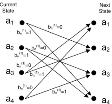
a1
•
•
•
•
•
•
•
•
bn(1)=0
a2
a3
a4
a1
a2
a3
a4 bn(1)=1
bn(1)=1 bn(1)=1
bn(1)=1 bn(1)=0
bn(1)=0 bn(1)=0 Current
State
Next State
Fig. 1. Miller Code State diagram.
The modulated signals are characterized by Discrete Time Markov Chains (DTMC) withRmstates, given by the PSK sym-bolsar ={Am·ej2π(r−1)/Rm
}, forr = 1,2, ..., Rm, whereAm is the amplitude of the signal of themthuser. The state transitions are defined by a block ofkmbits, denoted byBn ={b(1)n , b(2)n , ..., b(km)
n }, whereb(nk), fork=1, ..., km, is uniformly distributed over the set{0,1}and2km < Rm. In addition, it is assumed thatb(k)
n (k=1, ..., km) are mutually independent. For each of theRmstates, the block of bitsBndefines2km
equiprobable possible transitions. Therefore, the coding imposes some restrictions on the symbol tran-sitions. For each state, there is`
Rm−2km´
not assigned transi-tions. The code rate of themthuser is then given by (km/lm), wherelm= log2Rm.
Let us denote byT ={Tr1,r2}, withr1, r2 ∈ {1,2, ..., Rm}
the Transition Probability Matrix,Tr1,r2 being the probability of a
transition from the stater1to the stater2. Note thatPRr2m=1Tr1,r2 =
1andTr1,r2 ∈ {0,1/2
km}
. So, the matrixTdefines which are the possible state transitions for each state.
An example of mapping from the bits Bn to the correspond-ing PSK symbols is illustrated in Fig. 1 for a 4-PSK signal, where
{a1, a2, a3, a4}are the constellation symbols (states) andkm= 1.
This state diagram corresponds to the run-length-limited code known as Miller Code, associated with the transition probability matrix T2,B given in (13). The Miller Code widely used in digital mag-netic recording and in Binary-PSK carrier modulation systems [10]. Similar state diagrams can be obtained for the other transition prob-ability matrices given in the Appendix.
According to Theorem 2, if all the users transmit uniformly dis-tributed PSK signals, then conditions of Theorem 1 are verified for τ = 0. So, the following theorem proposes some constraints in the transition probability matrixTassociated with the users in such a way that all the users transmit uniformly distributed PSK signals.
Theorem 3: Let us assume that the DTMC associated with the coding is irreducible and aperiodic. IfPRm
r1=1Tr1,r2 = 1, for1≤
r2≤Rm, then, for a large number of time steps, the average fraction
of time steps during which the DTMC is in the statear1 converges
to1/Rm, for1≤r1≤Rm.
Proof: The aperiodicity and irreducibility properties assure that [15]: (i) all the limiting probabilities of a DTMC exist and are posi-tive, (ii) the stationary distribution exists and is unique, and (iii) the distribution of limiting probabilities is equal to the stationary distri-bution. So, the limiting probabilitiesP = [p1 p2 ... pRm]can be
obtained by the following system of equations
P T=P,
PRm
r=1pr= 1.
(6)
It can be easily verified that ifPRm
r1=1Tr1,r2 = 1, thenP= [1/Rm
...1/Rm]is a solution of the system (6). And finally, it can be proved (the proof is omitted due to a lack of space) that if the limiting probability of a statear1exists, then it is equal to the long-run time
average spent in the statear1, i.e. for a large number of time steps,
the average fraction of time steps that the DTMC spends in the state ar1converges to the limiting probability of the statear1.
In the sequel, some restrictions to the transition probability ma-trix are developed in order that the conditions of Theorem 1 are ver-ified forτ6= 0. LetTn
r1,r2be the(r1, r2)
thentry ofTn. By defini-tion,Tn
r1,r2represents the probability of being in the statear2after
ntransitions, supposing that the current state isar1. So, we may
write:
Ehskm(n+τ)slm(n)i= 1
Rma T
lTτak, (7)
wherea= [a1, a2, ... aRm]
Tanda
k=ˆak1, ak2, ... akRm ˜T
. Thus, the conditions (iii) and (iv) of Theorem 1 can be rewritten as:
aTTτa2= 0, aT2Tτa= 0 and aTTτa= 0. (8)
The results found in this section may be summarized in the following corollary.
Corollary 1: If the following conditions hold for all the users:
(i). the transition probability matrix corresponds to an irreducible and aperiodic DTMC;
(ii). PRm
r1=1Tr1,r2= 1,∀r2,1≤r2≤Rm;
and, in addition, equations (8) hold for(M−1)users∀τ ∈ Υ, then all the conditions of Theorem 1 are satisfied and, therefore, the covariance matrixC(τ)is diagonal∀τ∈Υ.
It should be highlighted that equations (8) only depend on the matrix Tand the constellation order. That means that transition probability matrices can be a priori designed to verify these equa-tions. In the Appendix, some examples of such matrices verifying these constraints are listed, with the corresponding admissible de-lays.
5. CHANNEL ESTIMATION ALGORITHM
Provided that the conditions of Corollary 1 hold, the channelHcan be estimated from the set of covariance matricesR(τ)by using a joint diagonalization algorithm. The proposed method can then be viewed as an extension of the SOBI algorithm [12] to nonlinear channels. The uniqueness of the joint diagonalizer based estima-tor is given by the following theorem [12]. The covariation matrix C(0)is assumed to be normalized, i.e.C(0) =IMV.
Theorem 4: LetB = {B1, ...,BT}be a set of T matrices MV ×MV such thatBt = MCtMH, for t = 1, ..., T, where M ∈ CMV×MV is a unitary matrix and C
t ∈ CMV×MV, for t = 1, ..., T, are diagonal matrices, the elements of which are de-noted byct(r) = [Ct]r,r. If
∃t ∈ {1, ..., T}such thatct(r1)6=ct(r2),
then any joint diagonalizer ofB is equal toΠΛM, whereΛis a diagonal matrix andΠa permutation matrix.
In the Appendix, some examples of configurations of transition probability matrices for 2 users are given, verifying the uniqueness condition (9). The estimation algorithm can be summarized as fol-lows:
(i). Calculate the whitening matrixUfrom:
U=
»
λ−
1 2
1 w1· · ·λ
−1 2
MV wMV –H
, (10)
where{λk}MV
k=1are theMV largest eigenvalues ofRˆ(0)and
{wk}Mk=1V, the corresponding eigenvectors, Rˆ(0)being the sampled estimate ofR(0). We have considered that the es-timated noise varianceσˆ2was already subtracted fromRˆ(0),
as mentioned earlier.
(ii). Calculate the following set of prewhitened matrices:
ˆ
RW(τ) = URˆ(τ)UH, forτ ∈ Υ, whereRˆ(τ)are the sam-pled covariance matrices.
(iii). Obtain a unitary matrixMˆ as the joint diagonalizer of the matricesRˆW(τ), forτ ∈Υ.
(iv). Estimate the channel matrix asHˆ=U†Mˆ and the transmitted signals asˆs(n) = ˆMHUx(n), where(·)†denotes the matrix pseudo-inverse.
Step (iii) of the method is carried out by using the joint diag-onalization algorithm of [11]. Note that the joint diagdiag-onalization estimator does not assume the knowledge of the covariance matrices of the sourcesC(τ)and that it requiresI≥MV.
6. SIMULATION RESULTS
In this section, the proposed nonlinear BSS and channel identifica-tion method is evaluated by means of computer simulaidentifica-tions with an uplink channel of a Radio Over Fiber (ROF) multiuser communica-tion system. The linear wireless interface is modeled as a memory-less multiuser channel. TheIantennae are half-wavelength spaced and the transmitted signals are narrowband with respect to the array aperture. Moreover, the propagation scenario is characterized by two users, the angles of arrival of which are30◦and70◦, respectively.
The E/O conversion in each antenna is modelled by the linear-cubic polynomialc1x+c3|x|2x, withc1=−0.291,c3= 1.078(see [4]).
The used modulation is 4-PSK and all the results were obtained via Monte Carlo simulations usingNR= 200independent data realiza-tions.
Fig. 2 shows the Normalized Mean Squared Error (NMSE) of the estimated transmitted symbols versus SNR for the configurations of transition probability matrices given in Table 1 of the Appendix, forM = 2,T = 4,Ns= 3000andI = 4, whereNsis the length of the data block used for the moment estimation. The NMSE of the transmitted signals is defined as:
eS(n) = 1
NR NR X
j=1
PNs
n=1ksj(n)−ˆsj(n)k 2 2
PNs
n=1ksj(n)k22
, (11)
wheresj(n)andˆsj(n)represents respectively the transmitted sig-nals and the estimated transmitted sigsig-nals at thejthMonte Carlo simulation andk · k2denotes thel2norm. The performance of our
technique is compared with that of the Minimum Mean Square Error
0 5 10 15 20 25 30 35 40 −40
−35 −30 −25 −20 −15 −10 −5 0 5
SNR (dB)
N
MSE
(d
B)
Config. 1 Config. 2 Config 3 Config 4 MMSE
Fig. 2. NMSE versus SNR for the configurations given in Table 1 -M= 2,T = 4,Ns= 3000andI= 4.
0 5 10 15 20 25 30 35 40 −35
−30 −25 −20 −15 −10 −5 0 5
SNR (dB)
N
MSE
−
C
h
a
n
n
e
l
Pa
ra
me
te
rs
(d
B)
Ns=100 Ns=300 Ns=500 Ns=1000 Ns=3000 Ns=5000 Ns=10000
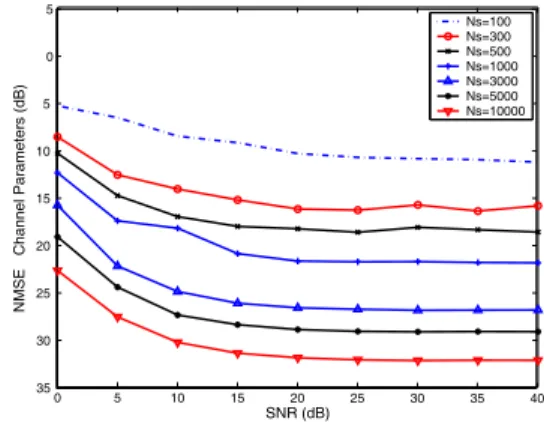
Fig. 3. NMSE of the channel parameters versus SNR for various values ofNsusing Config. 2,M = 2,T = 4andI= 10.
(MMSE) receiver [10] assuming perfect knowledge of the channel. Note that the tested configurations provide quite similar NMSE per-formances, not far from that of the MMSE receiver when the SNR is smaller than 25 dB.
Fig. 3 shows the NMSE of the channel parameters versus SNR for various values ofNs, where the NMSE of the channel parame-ters is defined as:eH= 1/NR“PNR
l=1kH−Hˆlk2F
”
/`
kHk2F
´
, wherek · kF denotes theFrobenius norm. In this case, we have used Config. 2 of Table 1,M = 2,T = 4andI = 10. It can be seen that the quality of the channel estimation can be considerably improved by increasing the length of the data block. This result in-dicates that the errors in the estimation of the covariance matrices constitute one of the main sources of performance degradation. In fact, if the theoretical values of the covariance matricesR(τ)are used, the estimation algorithm provides a very low NMSE for the estimated channel parameters, limited by the machine precision.
0 2 4 6 8 10 12 14 16 18 10−7
10−6 10−5 10−4 10−3 10−2 10−1 100
SNR (dB)
SER
Proposed − I=4 Proposed − I=8 MMSE − I=4 MMSE − I=8
Fig. 4. SER versus SNR using Config. 2,M = 2,T = 4and Ns= 3000, forI= 4andI= 8.
7. CONCLUSION
In this paper, the problem of BSS and channel identification for non-linear multiuser communication channels has been solved in assum-ing that the channel is modeled as a multiuser MIMO Volterra fil-ter. The proposed method is based on the joint diagonalization of a set of spatio-temporal covariance matrices. We have made use of modulation codes to ensure the orthogonality of nonlinear interfering terms for different time delays, which constitutes a new application of modulation codes. The proposed technique was tested by means of computer simulations with an uplink channel of a multiuser ROF communication system. In future works, other estimation algorithms will be tested and the impact of the modulation codes on the bit re-covery will be investigated.
A. APPENDIX - CONFIGURATIONS OF TRANSITION PROBABILITY MATRICES
As pointed out, the transition probability matrices can be a priori designed to verify the conditions of Corollary 1. In the following, we present some examples of such matrices corresponding to1/2 -rate codes for 4-PSK signals.
It can be proved by mathematical induction that the following matrices:
T1,A= 0.5
0
B @
1 1 0 0 0 1 1 0 0 0 1 1 1 0 0 1
1
C
A,T1,B= 0.5 0
B @
0 1 1 0 0 0 1 1 1 0 0 1 1 1 0 0
1
C A,
(12) verify all the conditions of Corollary 1∀τ ∈ I. In this casea = [1j −1 −j]T. In addition,
T2,A= 0.5
0
B @
1 1 0 0 1 0 1 0 0 1 0 1 0 0 1 1
1
C
A,T2,B= 0.5 0
B @
0 1 0 1 0 0 1 1 1 1 0 0 1 0 1 0
1
C A.
(13) also verify conditions (i) and (ii) of Corollary 1.
The identifiability test indicated in Theorem 4 only depends on the covariance matricesC(τ), forτ ∈Υ, which can be calculated from the transition probability matrices by using (7) and:
Ehskm(n+τ)sl
∗
m(n)
i
= 1
Rma H
l Tτak. (14)
This means that, if the matricesTof the users are known, the iden-tifiability test can be carried out. Thus, it can be verified that the configurations of transition probability matrices for 2 users given in Table 1 verify the condition of Theorem 4. The corresponding ad-missible delays areΥ ={0,1, ..., T−1}, withT ≥2.
Table 1. Configurations of transition probability matrices for M=2.
Config. User 1 User 2
1 T1,A T2,B
2 T1,A T2,A
3 T1,B T2,B
4 T1,B T2,A
B. REFERENCES
[1] A. Ziehe, M. Kawanabe, S. Harmeling, and K.-R. Muller, “Blind sepa-ration of post-nonlinear mixtures using linearizing transformations and temporal decorrelation,” Journal of Machine Learning Research, vol. 4, no. 7-8, pp. 1319–1338, 2003.
[2] S. Z. Pinter and X. N. Fernando, “Estimation of radio-over-fiber up-link in a multiuser CDMA environment using PN spreading codes,” in
Canadian Conf. on Elect. and Computer Eng., May 1-4, 2005, pp. 1–4. [3] X. N. Fernando and A. B. Sesay, “Higher order adaptive filter based predistortion for nonlinear distortion compensation of radio over fiber links,” inProc. of the Intern. Conf. on Communications (ICC’ 2000), vol. 1/3, New-Orleans, LA, USA, June 2000, pp. 367–371.
[4] X. N. Fernando and A. B. Sesay, “A Hammerstein-type equalizer for concatenated fiber-wireless uplink,” IEEE Trans. on Vehicular Tech-nology, vol. 54, no. 6, pp. 1980–1991, 2005.
[5] W.I. Way, “Optical fiber based microcellular systems. An overview,”
IEICE Trans. Commun., vol. E76-B, no. 9, pp. 1091–1102, Sept. 1993. [6] C. Jutten, M. Babaie-Zadeh, and S. Hosseini, “Three easy ways for separating nonlinear mixtures?,” Signal Processing, vol. 84, no. 2, pp. 217–229, Feb. 2004.
[7] A. Taleb and C. Jutten, “Source separation in post-nonlinear mixtures,”
IEEE Trans. on Sig. Proc., vol. 47, no. 10, pp. 2807–2820, Sept. 1999. [8] S. Harmeling, A. Ziehe, M. Kawanabe, and K.-R. Muller, “Kernel-based nonlinear blind source separation,”Neural Comp., vol. 15, no. 5, pp. 1089–1124, May 2003.
[9] A. J. Redfern and G. T. Zhou, “Blind zero forcing equalization of mul-tichannel nonlinear CDMA systems,” IEEE Trans. on Sig. Proc., vol. 49, no. 10, pp. 2363–2371, Oct. 2001.
[10] J. G. Proakis, Digital Communications, McGraw-Hill, 4rdedition, 2001.
[11] J.-F. Cardoso and A. Souloumiac, “Jacobi angles for simultaneous di-agonalization,” SIAM Journal on Matrix Anal. and Applicat., vol. 17, no. 1, pp. 161–164, Jan. 1996.
[12] A. Belouchrani, K. Abed-Meraim, J.-F. Cardoso, and E. Moulines, “A blind source separation technique using second-order statistics,” IEEE Trans. on Sig. Proc., vol. 45, no. 2, pp. 434–444, Feb. 1997.
[13] I. B. Djordjevic, B. Vasic, and V. S. Rao, “Rate 2/3 modulation code for suppression of intrachannel nonlinear effects in high-speed optical transmission,”IEE Proc.-Optoelectron., vol. 153, no. 2, pp. 87–92, Apr 2006.
[14] Y. Rong, S. A. Vorobyov, A. B. Gershman, and N. D. Sidiropoulos, “Blind spatial signature estimation via time-varying user power loading and parallel factor analysis,”IEEE Trans. on Signal Proc., vol. 53, no. 5, pp. 1697–1709, May 2005.