Blind of multiuser nonlinear channels using tensor decomposition and precoding

(1)

Blind identiﬁcation of multiuser nonlinear channels using tensor

decomposition and precoding

$

Carlos Alexandre Fernandes

a,b

_{, Ge´rard Favier}

a,

_{, Joa˜o Cesar M. Mota}

b

a_{I3S Laboratory, University of Nice-Sophia Antipolis/CNRS, Les Algorithmes/Euclide B-2000, route des Lucioles, BP 121, 06903 Sophia-Antipolis Cedex, France} b_{Departamento de Engenharia de Teleinforma}_{´tica, Federal University of Ceara´, Campus do Pici, 60.755-640, 6007 Fortaleza, Brazil}

a r t i c l e

i n f o

Article history:

Received 10 April 2008 Received in revised form 16 February 2009 Accepted 7 May 2009 Available online 23 May 2009

Keywords:

Blind nonlinear channel identiﬁcation Markov chain

Multiuser channel PARAFAC decomposition Volterra model

a b s t r a c t

This paper presents two blind identiﬁcation methods for nonlinear memoryless channels in multiuser communication systems. These methods are based on the parallel factor (PARAFAC) decomposition of a tensor composed of channel output covariances. Such a decomposition is possible owing to a new precoding scheme developed for phase-shift keying (PSK) signals modeled as Markov chains. Some conditions on the transition probability matrices (TPM) of the Markov chains are established to introduce temporal correlation and satisfy statistical correlation constraints inducing the PARAFAC decom-position of the considered tensor. The proposed blind channel estimation algorithms are evaluated by means of computer simulations.

1. Introduction

Two blind identification methods for multiuser non-linear communication channels are proposed in the present paper. The considered channel is represented by means of a memoryless multiple-input–multiple-output (MIMO) Volterra model. This kind of nonlinear models has important applications in the field of telecommunications, e.g. to model MIMO satellite communication channels with nonlinear power amplifier (PA). Due to power limitation, the satellite station usually employs a PA that is driven at or near saturation in order to obtain a power efficient transmission[1,2]. At saturation, the PA exhibits a nonlinear characteristic, resulting in the introduction of nonlinear bandlimited distortions[3].

MIMO Volterra models are also used for modeling uplink channels in radio over fiber (ROF) multiuser communication systems[4,5]. The ROF links have found a new important application with their introduction in microcellular wireless networks. In such systems, the uplink transmission is carried out from a mobile station toward a radio access point, the transmitted signals being converted in optical frequencies by a laser diode and then retransmitted through optical fibers. Important nonlinear distortions are introduced by the electrical–optical (E/O) conversion[4,6,7]. When the length of the optical fiber is short (few kilometers) and the radio frequency has an order of GHz, the dispersion of the fiber is negligible[8]. In this case, the nonlinear distortion arising from the E/O conversion process becomes preponderant. Up to several Mbps, the ROF channel can be considered as a memoryless link[6]. Thus, the channel is composed of a wireless link, modeled as a linear instantaneous mixture, followed by the E/O conversion, modeled as a memoryless nonlinearity. The overall channel can then be viewed as a memoryless MIMO Wiener filter, corresponding to a particular case of MIMO Volterra filters.

Contents lists available atScienceDirect

journal homepage:www.elsevier.com/locate/sigpro

Signal Processing

$

This research was supported by the CAPES/COFECUB project no. 544/7

_{Corresponding author. Tel.: +33 492942736; fax: +33 492942896.}

(2)

There are few works dealing with the problem of blind channel identiﬁcation or source separation in the context of multiuser or MIMO nonlinear communication systems. Ref. [9] proposed a blind zero forcing receiver for multiuser code division multiple access (CDMA) systems with nonlinear channels and Ref.[10]developed blind and semi-blind source separation algorithms for memoryless Volterra channels in ultra-wide-band systems.

The proposed channel identiﬁcation methods rely on the parallel factor (PARAFAC) decomposition [11]

of a tensor (multidimensional array) composed of spa-tio-temporal covariances of the signals received by an antenna array. A great advantage of using the PARAFAC decomposition is that it allows to work when the number of receive antennas is smaller than the number of virtual sources, i.e. the number of nonlinear terms of the Volterra ﬁlter. This is particularly interesting since Volterra ﬁlters may have a large number of parameters. Indeed, working with a number of receive antennas higher than or equal to the number of virtual sources imposes a strong constraint on the number of antennas to be used; see previous works

[5,9,12–14].

In telecommunications, the transmitted signals are usually assumed to be white. Thus, if we intend to exploit the temporal correlation of the sources for estimating the channel, some strategy must be used to induce correlation on the transmitted signals. It is shown that the input signals must satisfy some orthogonality constraints associated with the channel nonlinearities in order to get the PARAFAC decomposition of the considered tensor. A precoding scheme is then proposed so that these constraints be satisﬁed. In this scheme, transmitted signals are modeled as discrete time Markov chains (DTMC) inducing temporal correlation in a controlled way and some orthogonality properties. The proposed precoding scheme induces correlation by introducing redundancy on the signals, which is carried out by imposing some constraints on the symbol transitions. In fact, the proposed transmission scheme can be viewed as a special case of differential encoding. The introduction of redundancy in the transmitted signals is sometimes used with bandwidth-constrained channels, where a perfor-mance gain can be achieved without expanding the channel bandwidth or the transmission power[15]. Some properties of nonlinearly distorted PSK signals established in Ref.[13]have motivated the use of phase-shift keying (PSK) signals in the present work.

Two algorithms are proposed to perform channel estimation: a two-step version of the alternating least squares (ALS) algorithm[11,16]and a joint diagonalization algorithm (JDA) [17,18]. The second estimation method can be viewed as an extension of the second-order blind identiﬁcation (SOBI) algorithm [18] to nonlinear channels. The SOBI algorithm is a blind source separation and identiﬁcation technique for linear memoryless mix-tures based on the joint diagonalization of covariance matrices, and exploiting the temporal correlation of the sources.

Second-order statistics have been used for blind identiﬁcation and equalization of nonlinear single-input– multiple-output channels (SIMO) [12,14,19].

PARAFAC-based blind channel identiﬁcation and source separation have also been addressed in the case of linear channels in the context of CDMA systems [16,20–23]. In Ref. [24], a time-varying user power loading was proposed to enable the application of the PARAFAC analysis, in order to perform blind estimation of spatial signatures. Blind source separation using a PARAFAC tensor composed of covariance matrices was also proposed in Ref.[25]. In the case of nonlinear channels, a deterministic blind PARAF-AC-based receiver was presented for SIMO channels in Ref.

[26] and a blind identiﬁcation method based on the PARAFAC decomposition of a channel output data tensor was recently proposed for Wiener–Hammerstein type channels[27].

The rest of this paper is organized as follows. Section 2 presents the channel model used in this work. In Section 3, a tensor composed of channel output covariances is introduced. In Section 4, some orthogonality constraints are established to get a PARAFAC decomposition of this tensor. In Section 5, these constraints are rewritten in terms of the transition probability matrix (TPM) of a Markov chain and a procedure to design TPMs satisfying such constraints is described. Section 6 presents the pro-posed blind channel estimation algorithms. In Section 7, we evaluate the performance of these algorithms by means of simulation results. Finally, some conclusions and perspec-tives are drawn in Section 8.

2. The channel model

The sampled baseband equivalent model of the non-linear communication channel is assumed to be expressed as a truncated MIMO Volterra series:

yrðnÞ ¼

XK

k¼0

XT

t1¼1 X

T

tkþ1¼tk

XT

tkþ2¼1 X

T

t2kþ1¼t2k

|fflfflfflfflfflfflfflfflfflfflfflffl{zfflfflfflfflfflfflfflfflfflfflfflffl}

ftkþ2;...;t2kþ1g\ft1;...;tkþ1g¼;

hð₂r_kÞ_þ₁ðt1;. . .;t2kþ1Þ

Y

kþ1

i¼1 stiðnÞ

Y

2kþ1

i¼kþ2 s

tiðnÞ þ

ur

ðnÞ, (1)

whereyrðnÞ ð1rRÞis the signal received by antennar at the time instantn,Ris the number of receive antennas, ð2Kþ1Þis the nonlinearity order of the model,stðnÞ ð1 tTÞ is the stationary signal transmitted by the tth user at the time instant n, T is the number of users, hð₂r_kÞ_þ1ðt1;. . .;t2kþ1Þ are the coefﬁcients of the ð2kþ 1Þth-order Volterra kernel of therth sub-channel and

ur

ðnÞis the zero-mean additive white Gaussian noise (AWGN), with variance

s

2_for_r_¼_1;_2;_{. . .}_;_R.

(3)

user indextis omitted from these parameters. Besides, it is assumed that

P42K_þ1, (2)

which corresponds to the well-known persistence of excita-tion condiexcita-tion for a Volterra system of orderð2Kþ1Þ[28].

The nonlinear terms corresponding toti¼tj, for alli2 f1;. . .;kþ1gand j2 fkþ2;. . .;2kþ1g, are absent in (1) due to the fact that, for constant modulus signals, the term jstiðnÞj

2 _{reduces to a multiplicative constant that can}

be absorbed by the associated channel coefﬁcient. As a consequence, some nonlinear terms degenerate in terms of smaller order. Besides, the equivalent baseband Volterra model (1) includes only the odd-order kernels with one more non-conjugated term than conjugated terms because the other nonlinear products of input signals correspond to spectral components lying outside the channel bandwidth, and can therefore be eliminated by bandpass ﬁltering[29,30].

The matrix representation of (1) is given by

yðnÞ ¼HwðnÞ þvðnÞ, (3)

where yðnÞ ¼ ½y1ðnÞ;. . .;yRðnÞT 2

C

R1 _{is the received}

wðnÞ,˜ (4)

where

˜

wðnÞ ¼ ½sT_ðnÞ3

s

T_ðnÞ2Kþ1

s

T_ðnÞT_, ₍₅₎

with sðnÞ ¼ ½s1ðnÞ;. . .; sTðnÞT2

C

T1 and the operator

2kþ1

deﬁned as

2kþ1

sðnÞ ¼ ½

kþ1_{sðnÞ ½}k_s_ðnÞ, ₍₆₎

denoting the Kronecker product and k_{sðnÞ ¼}

sðnÞ sðnÞ, with k1 Kronecker products. The

matrix

Y

is a row-selection matrix that selects all the elements of wðnÞ˜ corresponding to Qk_i_¼1þ1stiðnÞ

Q2kþ1 i¼kþ2stiðnÞ

with t1 tkþ1, tkþ2 t2kþ1 and ftkþ2;. . .; t2kþ1g \ ft1;. . .;tkþ1g ¼ ;, fork¼1;2;. . .;K.

3. PARAFAC decomposition of a channel output covariance tensor

The proposed identiﬁcation methods rely on the PARAFAC decomposition of a tensor composed of spatio-temporal covariances of the received signals. Assuming

that these signals are stationary and ergodic, we have

RyðdÞ ¼

E

½yðnþdÞyHðnÞ ¼HRwðdÞHHþ

s

2IR

dðdÞ 2

C

RR, (7)

with

RwðdÞ ¼

E

½wðnþdÞwHðnÞ 2

C

QQ, (8)

where 0dD1,Dis the number of delays (time lags) taken into account,

dðÞ

is the Kronecker symbol,IR is the identity matrix of orderR,

E

_½:denotes the mathematical expectation and the superscriptHstands for the complex conjugate transpose (Hermitian transpose). In the sequel, it is assumed that the noise variance

s

2 _{is known,} allowing the subtraction of the noise term in (7). Then, from now on, the noise term will be omitted. However, in practice, this noise variance has to be estimated[18,31]or the proposed identiﬁcation methods can be applied without using the zero-lag covariance matrixðd¼0Þ.

A third-order tensor

R

₂

C

DRR

can be deﬁned from the matricesRyðdÞ, with

rd;r1;r2¼

E

½yr1ðnþd1Þy

r2ðnÞ, (9)

as entries, for 1dD and 1r1;r2R. From (7), we get

rd;r1;r2¼

XQ

q1¼1

XQ

q2¼1 hr1;q1h

r2;q2˜rd;q1;q2, (10)

where hr;q¼ ½Hr;q and ˜rd;q1;q2¼

E

½wq1ðnþd1Þw

q2ðnÞ, wqðnÞ ðq¼1;. . .;QÞ being the qth component of the nonlinear input vector wðnÞ. Note that Eq. (10) corre-sponds to the scalar writing of a Tucker2 model[32].

Definition 1. Let

X

2

C

IJK

be a third-order tensor with entries xi;j;k, for 1iI, 1jJ and 1kK. The PARAFAC decomposition of the tensor

X

is given by

xi;j;k¼

XQ

q¼1

ai;qbj;qck;q, (11)

where ai;q, bj;q and ck;q are the elements of the matrix factorsA2

C

IQ_,_B₂

C

JQ_and_C₂

C

KQ_{, and}_Q_{is the rank} of

X

.

If the covariance matrices Rwðd1Þ of the nonlinear input vector are diagonal for 1dD, the scalar writing (10) of

R

becomes

rd;r1;r2¼

XQ

q¼1

cd;qhr1;qhr2;q, (12)

which corresponds to the PARAFAC decomposition of

R

with factor matrices equal toC,HandH_{, the matrix}_C₂

C

DQbeing formed with the diagonal elements ofRwðd1Þ for 1dD, i.e.

C¼

˜r1;1;1 ˜r1;Q;Q

. .

. _.

.

. _.

. .

˜rD;1;1 ˜rD;Q;Q

2 6 6 4

3 7 7

5, (13)

(4)

veriﬁed[33]:

2kHþkC2Qþ2, (14)

wherekAis the k-rank of matrixA, i.e. the greatest integer kA such that every set of kA columns of A is linearly independent. The essential uniqueness property means that the matricesH,H_and_C_{are unique up to column scaling} and permutation ambiguities, i.e. any matrices_H^

a,H^bandC^ satisfying (12) are linked toH,H andCby_H^

a¼HPLa, ^

is aQ Q permutation matrix.

Assuming that the matricesHandCare full k-rank, i.e. kH¼minðR;QÞ and kC¼minðD;QÞ, Kruskal’s condition becomes 2minðR;QÞ þminðD;QÞ 2Qþ2, which implies that the tensor approach allows working even if RoQ, contrarily to previous works that require RQ [5,9,12–14]. This is particularly interesting for identifying Volterra systems characterized by a large number of parameters.

In the next section, we establish some conditions for ensuring that the covariance matricesRwðdÞbe diagonal for 0dD1, in order to get a PARAFAC decomposi-tion of the tensor

R

.

4. Orthogonality conditions

The following theorem states sufﬁcient conditions to ensure that the covariance matrices of the non-linear input vectorRwðdÞ(0dD1) be diagonal when the transmitted signals are PSK modulated.

½sitðnþdÞs j

tðnÞ. (16)

Proof. The elements of Rwðd1Þ (1dD) are

deﬁned as

˜rd;q1;q2¼

E

½wq1ðnþd1Þw

q2ðnÞ, (17)

wherewq1ðnÞandwq2ðnÞcan be written, respectively, as

wq1ðnÞ ¼

YT

t¼1 sat

t ðnÞ½sbttðnÞ, (18)

wq2ðnÞ ¼

YT

t¼1 sa0t

t ðnÞ½s

b0 t

t ðnÞ, (19)

for some non-negative integers

at

;

b

a

0

t¼k 0

þ1 and X T

t¼1

b

0t¼k

0_. ₍₂₀₎

Note that, due to the circularity property of PSK signals, we have sP

0t(or both), for allt¼1;. . .;T. Hence, (18) and (19) can be rewritten, respectively, as

wq1ðnÞ ¼

YT

t¼1 _ sgt

t ðnÞ and wq2ðnÞ ¼

YT

t¼1 € sg0t

t ðnÞ, (21)

(

(22)

Substituting (21) into (17), we get

˜rd;q1;q2¼

YT

t¼1

E

_½_s_gt

t ðnþd1Þ½s€

g0 t

tðnÞ. (23)

Ifq₁aq₂, there are at least two userst1 andt2 such that ð

at

1;

b

t1Það

a

0 t1;

b

0

t1Þandð

at

2;

b

t2Það

a

0 t2;

b

0

t2Þ. Thus, (23) can be rewritten as

˜rd;q1;q2¼

YT

t¼1

tat1;t2

E

_½_s_gt

t ðnþd1Þ½€s

g0 t tðnÞ

E

½_s

gt1

t1ðnþd1Þ

½€_sg 0 t1

t1ðnÞ

_E

_½__sgt2

t2ðnþd1Þ½ € sg

0 t2

t2 ðnÞ

_. ₍₂₄₎

Depending on the different possible conﬁgurations of the couplesð_s__t

1ðnÞ;s€t1ðnÞÞandð_st2ðnÞ;€st2ðnÞÞ, the two last factors of (24) can be expressed in terms of the following quantities:

m

ði;jÞ

t ðd1Þ, with 0i;jKþ1 andiaj;

R

ði;jÞ

t ðd1Þ, with 1iKþ1, 1jK;

(5)

To illustrate Theorem 1, let us consider the covariance matrixRwðdÞfor two usersðT¼2ÞandK¼1, given by

and associated with the following nonlinear input vector:

wðnÞ ¼ ½s1ðnÞ s2ðnÞ s21ðnÞs2ðnÞ s1ðnÞ s22ðnÞ. (25)

Note that all the off-diagonal components ofRwðdÞare the product of two terms like (15) and (16), witht¼1 or 2. Then, if conditions (i) and (ii) hold for at least one user, the matrixRwðdÞis diagonal.

5. Transmitted signal design

In this section, a precoding scheme is proposed so that the transmitted signals satisfy the orthogonality con-straints of Theorem 1. Each transmitted signal is modeled as a DTMC, the states of the DTMC being given by the P-PSK symbolsap¼A ej2pðp1Þ=P;p¼1;2;. . .;P. The coding induces time correlation by introducing redundancy on the signals, which is done by imposing some constraints on the TPM associated with the DTMC. The correlation is introduced in a controlled way so that the constraints of Theorem 1 are satisﬁed, the TPM playing a key role in this scheme.

Let us denote byLB the number of input bits of the encoder, assumed to be independent and identically distributed (i.i.d.) and uniformly distributed over the set f0;1g. Moreover, we assume that L¼2LB_o_{P, which}

imposes some restrictions on the symbol transitions. This means that, for each state, there are L equiprobable possible transitions and ðPLÞnot assigned transitions. The code rate is therefore equal toLB=log2P.

Let us denote byT¼ fTp1;p2g, withp1;p22 f1;2;. . .;Pg, the TPM for a given user, Tp1;p2 being the probability of transition from the stateap1to the stateap2. Each user is associated with a different TPM. However, for simplifying the notation, the user indextwill be omitted fromT. Note

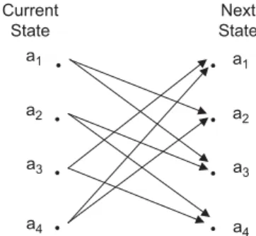
that PPp2¼1 Tp1;p2¼1, for 1p1P. Hence, each row of the TPM hasL¼2LB _{elements equal to 1=L}_¼₂LB_and

ðPLÞelements equal to zero. For instance,Fig. 1shows the state transition diagram of a DTMC corresponding to P¼4 andLB¼1, with the following TPM:

T¼1

2

0 1 1 0

0 0 1 1

1 0 0 1

1 1 0 0

2 6 6 6 4

3 7 7 7 5

. (26)

5.1. Orthogonality constraints in terms of the TPM

The orthogonality constraints of Theorem 1 are now rewritten in terms of the TPMTof the DTMC associated with each user. Some important properties of DTMC are ﬁrst recalled [34]. In what follows, Tn;p1;p2 denotes the ðp1;p2Þelement ofTn, which represents the probability of being in the stateap2 aftern transitions, supposing that the current state isap1.

Definition 2. A stateapof a DTMC is said to beaperiodicif

the great common divisor of the set of integersnsuch that Tn;p1;p240 is equal to 1. If all the states are aperiodic, then the DTMC is also aperiodic.

Definition 3. A stateap2of a DTMC is said to beaccessible

from the stateap1if there exists some integernsuch that Tn;p1;p240.

Definition 4. A DTMC is said to be irreducibleif all the

states are accessible from each other.

Definition 5. The limiting probability

y

p2ð1p2PÞof a

given state of a DTMC is deﬁned as

y

p2¼_nlim_!1Tn;p1;p2;8p12 f1;2;. . .;Pg. (27)

Definition 6. A probability distribution

P

¼ ½

p

1;

p

2;. . .;

pP

, 0

p

1;. . .;

pP

1, is stationary if the following conditions are satisﬁed:

PT

¼

P,

(28)

XP

p¼1

pp

¼1. (29)

Definition 7. An irreducible and aperiodic DTMC is said to

be stationary if the initial state is chosen according to the stationary distribution.

In what follows, we reformulate the conditions of Theorem 1 in terms of the TPM of a given user. For that, we ﬁrst establish in Lemma 1 the conditions to be a1

• •

•

• •

•

• a2

a3

a₄

a1

a₂

a₃

ð1;2Þ

2 ðdÞ

½

R

ð1;1Þ 1 ðdÞ

m

ð2

;0Þ 2 ðdÞ

m

ð0

;1Þ 1 ðdÞ

m

ð2

;1Þ

2 ðdÞ ½

R

ð1

;2Þ 1 ðdÞ

R

quan-tities(15)and(16)can be rewritten as

m

ði;jÞ_{ðdÞ ¼}1 P½a

j

HTdaj ₍₃₁₎

and

R

ði;jÞ_{ðdÞ ¼}1 P½a

jT_Td_ai_, ₍₃₂₎

wherea¼ ½a1;a2;. . .;aPTandai¼ ½ai₁;ai₂;. . .;aiP T_.

Proof. From Lemma 1, conditions C1–C3 ensure that

the DTMC is stationary with a uniform distribution. Thus, we get

m

ði;jÞ_{ðdÞ ¼}

_E

_½si

ðnþdÞ½sjðnÞ_¼X P

p1¼1

XP

p2¼1

pð

an

¼ap1Þ½a

j p1

_T

d;p1;p2a

i p2

¼ 1 P½a

j

HTdai_. ₍₃₄₎

Expression (32) can be derived in a similar way. &

Remark. Note that, when i or j¼0, condition (i) of

Theorem 1 becomes

E

½si_{ðnÞ ¼}_0, ₍₃₅₎

for 1iKþ1. On the other hand, ford¼0, condition (i) becomes

m

_½si_{ðnÞ ¼}A i

P

XP

p¼1

ej2pðp1Þi=P_¼ A i

ðej2pi_1Þ

Pðej2pi=P_1Þ¼0, (37)

for 1iKþ1oP, we can conclude that condition (i) of

Theorem 1 is satisﬁed ford¼0, andiorj¼0.

In summary, combining Lemma 1, Theorem 2 and the above remark, the conditions of Theorem 1 can be reformulated as follows:

(C1) the DTMC is irreducible and aperiodic; (C2) PP_p

2¼1Tp1;p2¼1, for 1p1P; (C3) PPp1¼1Tp1;p2¼1, for 1p2P; (C4) ½aj

HTdai_¼_{0, for all}_i_and_j_{such that 1}_i;_j_K_þ₁ withiaj;

(C5) ½ajT_Td

ai_¼_{0, for all}_i_and_j_{such that 1}_i_K_þ_1, 1jK;

for 1dD1 and at leastðT1Þusers.

5.2. Determination of the transition probability matrices

For a given user, conditions C2 and C3 can be written as the following set of linear equations:

Y

3

Y

4

Y

4¼ ½IP10P1ðIP1TPÞ, (40)

(7)

The sum of the elements of the last column of Tis not included as it represents a redundant constraint.

Moreover, for allði;jÞsuch that 1i;jKþ1, condi-tions C4 and C5 can be written in a matrix form, respectively, as

AHTdA¼0ðKþ1ÞðKþ1Þ and ATTdA¼0ðKþ1ÞðKþ1Þ, (41)

where

A¼ ½a a2_aKþ1₂

_C

PðKþ1Þ_. ₍₄₂₎

Applying the vecðÞ operator to the two members of Eq. (41) and using the following property, vecðABCÞ ¼

22

R

ðK

2

þKÞðKþ1Þ2

is a row selection matrix that eliminates the rows ofðAT ATÞcorresponding toðaT

i a T

Kþ1Þ, fori¼1;2;. . .;Kþ1. Thus, the TPMs must satisfy (38) and (45) and condition C1. It should be highlighted that, once chosen the values ofK,PandLB, these constraints only depend on the matrixT, which means thatTcan be a priori designed. By exploiting the fact that Tp1;p22 f0;1=Lg, the next theorem proposes a procedure to determine TPMs that verify (38) and (45) for any values ofK,PandLB.

Definition 8. The pth circulant diagonal (p¼1;. . ._;P)

of a PP matrix is the set of entries corresponding to the following indices: ðk;modðpþk2;PÞ þ1Þ, for k¼1;. . ._;P, where modð;PÞ denotes the modulo opera-tion, i.e. the remainder of the division of the argument by P.

Definition 9. Let us deﬁne TPðp1;. . .;pLÞ as the PP

matrix having entries equal to 1=L on the circulant diagonals p1;. . .;pL and to zero elsewhere, with L¼2LB_o_P.

For instance, forP¼4 andLB¼1 (L¼2), the TPM (26) is denoted byT4ð2;3Þ.

Theorem 3. The matricesTPðp1;. . .;pLÞsatisfy(38)and(45)

for all1p1op₂o op_LP.

Proof. Each row and column of TPðp1;. . .;pLÞcontains L

elements equal to 1=LandðPLÞelements equal to zero. Hence, conditions C2 and C3, i.e. Eq. (38), are always satisﬁed. In the sequel, it is proved thatTPðp1;. . .;pLÞalso satisﬁes condition C4 for alld1.

Ford1, deﬁningq¼Tai

2

C

P1, condition C4 can be rewritten as

½aj

HTdai_{¼ ½a}j

HTd1q. (46)

The ﬁrst element of the vectorqcan be developed as

q1¼

XP

p¼1 T1;paip¼

XL

l¼1 T1;pla

i pl¼

1 L

XL

l¼1 ai

pl. (47)

By using Deﬁnition 8, thekth element (k¼2;. . .;P) ofq can be expressed as

qk¼

XP

p¼1 Tk;paip¼

XL

l¼1

Tk;½modðplþk2;PÞþ1a

i

½modðplþk2;PÞþ1.

(48)

For PSK modulated symbols, we have

ai

½modðplþk2;PÞþ1¼A

i_ej2p½modðplþk2;PÞi=P_¼_Ai_ej2pðplþk2Þi=P

¼a i pla

i k

Ai . (49)

Substituting (49) into (48) gives

qk¼ 1 LAi

XL

l¼1 ai

pla i k¼

ai kq1

Ai . (50)

Thus, the vectorqcan be written as

q¼Tai

¼q1 Aia

i_. ₍₅₁₎

By substituting (51) into (46), we get the following recursive equation:

½aj

HTdai_¼q1 Ai½a

j

HTd1ai_, ₍₅₂₎

which leads to

½aj

HTdai_¼ q1 Ai

d ½aj

Hai

¼ q1 Ai

d AiþjX

P

p¼1

ej2pðp1ÞðijÞ=P

¼ q1 Ai

d

Aiþj ej2pðijÞ1

ej2pðijÞ=P₁, (53)

which is equal to zero for iaj. That proves that the matricesTPðp1;. . .;pLÞsatisfy condition C4. A similar proof can be made for condition C5. &

(8)

can be veriﬁed that the matrices T4ð1;3Þ and T4ð2;4Þ correspond, respectively, to a reducible and a periodical DTMC. Thus, for 4-PSK signals, the matrices T4ð1;2Þ, T4ð2;3Þ,T4ð3;4ÞandT4ð1;4Þare the only matrices satisfy-ing the orthogonality conditions C1–C5.

5.3. Interpretation of the TPM

An interesting characteristic of the matrixTPðp1;. . .;pLÞ is that the corresponding precoding can be viewed as a differential coding. For a given row ofTPðp1;. . .;pLÞ, each non-zero element is associated with one of the L combinations of the LB input bits of the encoder. From Deﬁnition 8, the difference between the row and the column indices of an element of thepth circulant diagonal (1pP) is given byðmodðp2;PÞ þ1Þ ¼p1, which means that all thePelements of thepth circulant diagonal correspond to the same phase shift 2

p

ðp1Þ=P. Thus, if we associate all the P elements of the pth circulant diagonal to the same combination of theLBinput bits, this combination will be associated with the same phase shift, regardless of the input state. The symbols may then be decoded using only the difference of phase of two consecutive symbols, which is the principle of a differ-ential coding. This characteristic simpliﬁes the decoding process and makes it insensitive to scaling ambiguities.

The difference between the proposed coding and the conventional differential coding is that, in the proposed approach, there are some phase shifts that are not allowed. The allowed phase shifts are determined by the circulant diagonals of the TPM, the circulant diagonal p corresponding to a phase shift of ð2

p

ðp1Þ=PÞ. For instance, let us consider the TPM T4ð2;3Þ, given in (26), and corresponding to the state transition diagram shown inFig. 1. If the bit mapping deﬁned inTable 1is used, the symbols may then be decoded from the phase shift of two consecutive symbols: if this phase shift is equal to

p

=2 (resp.

p

), the input bit of the encoder is equal to 0 (resp. 1). The choice of the circulant diagonals determines two characteristics of the coding: the distance between the possible phase shifts and the induced correlation. With respect to the ﬁrst characteristic, it is desirable to choose the circulant diagonals so that the distance between the allowed phase shifts 2

p

ðp1Þ=Pbe high, due to the fact that close phase shifts are more difﬁcult to recover in the presence of noise and interference. For instance, forP¼8 andLB¼1, it is easy to verify that the matricesT8ði;iþ3Þ ð1i8Þ provide the maximal euclidean distance be-tween the allowed phase shifts. Note that the matrices

T8ði;iþ4Þ ð1i8Þ correspond to reducible DTMCs. Moreover, forP¼8, LB¼2 and considering only irredu-cible and aperiodic DTMCs, we found by an exhaustive search for all the values of p₁;p₂;p₃;p₄ such that 1p1op₂op₃op₄8, that the TPMs maximizing the

RDRthe ﬁrst- and third-mode unfolded matrices of the tensor

R

, deﬁned as

R1

. . .

RD

2 6 6 4

3 7 7 5; R3

R1

. . .

RR

2 6 6 4

3 7 7

5. (55)

These matrices are given by

R1¼ ðCHÞHH and R3¼ ðH_CÞHT_, ₍₅₆₎

wheredenotes the Khatri–Rao (column-wise Kronecker) product:

CH¼

Hdiag₁½C

. . .

HdiagD½C

0 B B @

1 C C

A. (57)

6.1. Alternating least squares algorithm

The ﬁrst proposed channel estimation method uses a two-step ALS algorithm [11,16]. Indeed, the matrix Cis assumed to be known as it can be precomputed using the formula:

m

ði;iÞ_{ðdÞ ¼}1 P½a

i

HTdai_, ₍₅₈₎

fori¼0;. . ._;Kþ1 andd¼1;. . ._;D.

The channel estimation problem is solved by minimiz-ing the two followminimiz-ing conditional least squares cost functions in an alternate way:

J1¼ kR1^ ðCH^ðait1ÞÞH^ T

bk2F; J2¼ kR3^ ðH^ð itÞ b CÞ

^ HTak2F,

(59)

where_R1^ _and_R3^ _{are, respectively, the sample estimates} of the unfolded matricesR1 andR3,itand k kF denote, respectively, the iteration number and the Frobenius norm. Two LS channel estimates, denoted by _H^ðitÞ

a and

Table 1

Bit mapping for the TPMT4ð2;3Þ.

Next state

Current state a1 a2 a3 a4

a1 Bn¼ f0g Bn¼ f1g

(9)

^ HðitÞ

b , corresponding, respectively, to estimates ofHandH

_,

are calculated at theitth iteration as

^ HðitÞ

b ¼ ½ðCH^

ðit1Þ

a ÞyR1^ T, (60)

^ HðitÞ

a ¼ ½ðH^

ðitÞ

b CÞ

y_R3^ T_, ₍₆₁₎

whereH^ð0Þa is chosen as anRQGaussian random matrix andðÞy_{denotes the matrix pseudo-inverse. The algorithm} iterates until the convergence of the estimated para-meters, i.e.

kH^ðitÞ ab

^ Hðit1Þ

ab k 2 F kH^ðit1Þ

ab k2F

o

, (62)

where

is an arbitrary small positive constant and ^

Hð_abitÞ¼0:5½_H^ðitÞ

a þ ðH^bðitÞÞ. The ALS algorithm is monotoni-cally convergent but it may require a large number of iterations to converge [35]. Three channel estimates can then be obtained:_H^ðitÞ

a ,ðH^

ðitÞ

b Þ

_{and 0:5½}_H^ðitÞ

a þ ðH^bðitÞÞ, the ﬁnal channel estimate being chosen as the one that provides the smallest value of the cost function (59). The ALS algorithm also works if the matrixCis unknown. In this case, three least squares estimates are calculated at each iteration.

6.2. Joint diagonalization algorithm

The channel matrixHcan also be estimated from the set of covariance matrices RyðdÞby JDA. Unlike the ALS algorithm, the joint diagonalization estimator requires RQ, i.e. it does not work in the underdetermined case. The estimation algorithm can be summarized as follows (for further details, see Ref.[18]):

(i) Calculate the whitening matrixUas

U¼ ½l1₁ =2u1

l

Q1=2uQH, (63)

whereflqgQ_q_¼1are theQ largest eigenvalues ofR^yð0Þ andfuqgQq¼1are the corresponding eigenvectors,R^yð0Þ being the sample estimate ofRyð0Þ. It is considered that the estimated noise variance

_s

^2_{was subtracted} from_R^

yð0Þ, as mentioned earlier.

(ii) Calculate the following set of prewhitened matrices: ^

RpðdÞ ¼UR^yðdÞUH, for 0dD1, where R^yðdÞ is the sample estimate ofRyðdÞ.

(iii) Determine an unitary matrix _M^ _{as the joint} diag-onalizer of the matrices_R^

pðdÞ, for 0dD1. (iv) Estimate the channel matrix as_H^ _¼_Uy_M.^

In the simulations of the next section, step (iii) of this method is carried out by using the joint diagonalization algorithm of Ref.[17]. Note that the JDA does not assume the knowledge of the source covariance matrix RwðdÞ. The resulting identiﬁcation method can then be viewed as an extension of the SOBI algorithm[18]to nonlinear channels.

7. Simulation results

In this section, the proposed channel estimation methods are evaluated by means of simulations. A memoryless linear-cubic MIMO Wiener model of an uplink channel of a radio over ﬁber multiuser commu-nication system[4,5]has been considered for the simula-tions. The wireless link is modeled as a Rayleigh RT linear channel, with an array ofRhalf-wavelength spaced antennas and T¼2 or 3 users. The E/O conversion in each antenna is modeled by the following polynomial c1xþc3jxj2x, withc1¼1 andc3¼ 0:35, as in Ref.[4,36]. The results were obtained with 8-PSK input signals (P¼8), via Monte Carlo simulations using at least 100 independent data realizations. The amplitude of the signals transmitted by all the users is equal to 1.

The proposed channel estimation methods are evalu-ated by means of the normalized mean square error (NMSE) of the estimated channel parameters, deﬁned as

NMSE¼ 1 NR

XNR l¼1

kHH^lk2F kHk2

F

, (64)

where_H^

lrepresents the channel matrix estimated at the lth Monte Carlo simulation after eliminating the ambi-guities. As a performance reference for the proposed channel estimation techniques, we also show the NMSE obtained with the Wiener solution, given by

^

H¼RywR^ 1ww¼Ryw,^ (65)

whereRyw^ is the sample estimate ofRyw¼E½yðnÞwH_ðnÞ, Rww¼E½wðnÞwH_{ðnÞ ¼}_I

Q andwðnÞis the nonlinear input vector deﬁned in (4). This non-blind solution needs to know the input signals.

Table 2describes the various tested simulation config-urations, the matricesT8ðp1;. . .;pLÞbeing constructed as in Definition 9. All the configurations ofTable 2provide matricesCsuch thatkC¼minðD;QÞ. Remark that Config-urations A, B, E and F correspond to a code rate of1

3while Conﬁgurations C and D lead to a code rate of 2

3. The circulant diagonals of the TPMs of Conﬁgurations B, D and F were chosen so that the correlation of the transmitted signals be maximized, this correlation being calculated using the following formula:

m

ð1;1Þ_{ðdÞ ¼}1 Pa

H_Td

Pðp1;. . .;pLÞa. (66)

If the induced correlation is low, the transmitted and received signals are ‘‘almost blind’’, which means that a

Table 2

Simulation conﬁgurations.

Conﬁg. T Q LB TPM of user 1 TPM of user 2 TPM of user 3

(10)

small value of D should be used due to an inaccurate estimation of the correlations_r^_d_;_r_1;_r

2. Thus, in general, for the purpose of channel estimation, it is desirable that this induced correlation be high. For instance, by an exhaus-tive search for all the values of p1;p2 such that 1p1op₂8, it can be concluded that, for P¼8 and

LB¼1, the matrices T8ði;iþ1Þ (1i8) provide the maximal time correlation, i.e. this choice of circulant diagonals maximizesPD1

d¼0j

m

ð1;1ÞðdÞj2, forD¼4. Similarly, forP¼8,LB¼2 andD¼4, the TPMs that maximize the time correlation areT8ði;iþ3;iþ4;iþ5Þ(1i8).

7.1. Simulations with a code rate of1 3

The next three figures compare the performance of the two proposed estimation algorithms using Configurations A and B ofTable 2, i.e. forT¼2 users and a code rate of1 3 (LB¼1). Fig. 2shows the NMSE versus signal-to-noise-ratio (SNR) provided by the ALS and JDA algorithms and by the Wiener solution, forR¼5,D¼4 and data blocks of N¼1024 symbols. It is also shown the NMSE obtained with the ALS algorithm in the case of Configuration B and an unknown noise variance (ALS-UNV), using covariances with delaysd¼1;2;. . .;4. The following conclusions can be drawn fromFig. 2:

Configuration B provides better performance than Configuration A, for both ALS and JDA algorithms. As pointed out earlier, this is probably due to the fact that Configuration B is the one that induces the highest correlation to the transmitted signals.

The performance of JDA is better than that of ALS, except when Conﬁguration B is used and the SNR is lower than 15 dB.

The NMSE provided by the ALS-UNV algorithm is approximatively 3 dB higher than the one obtained with the ALS algorithm.

JDA with Conﬁguration B performs better than the supervised Wiener solution when the SNR is higher

than 20 dB. This is due to the fact that the non-blind Wiener solution (65) does not exploit the time correlation of the transmitted signals, while the proposed estimation techniques do.

Fig. 3evaluates the performance of the proposed channel identiﬁcation methods in terms of bit-error-rate (BER). It shows the BER versus SNR provided by the minimum mean square error (MMSE) receiver:

^

WMMSE¼RwwH^H½HRww^ H^Hþ

s

2IR12

C

QR, (67)

using the ALS and JDA channel estimates, with Configura-tions A and B,R¼5,D¼4 andN¼1024. For comparison, it is also plotted the BER provided by the MMSE receiver assuming an exact knowledge of the channel, using Configuration A and differential binary PSK (DBPSK) input signals. The following conclusions can be drawn from this figure:

When JDA is used, Configuration A provides a lower BER than Configuration B. As pointed out earlier, this is certainly due to the distance of the allowed phase shifts of these configurations.

Using the ALS algorithm, Configuration A provides a lower BER than Configuration B when the SNR is smaller than 15 dB. This is due to the poor channel estimation performed by the ALS algorithm when Configuration A is used and to the fact that the multiuser interference is the main source of degrada-tion when the SNR is high.

Moreover, for a BER of 102_{and considering the case of} a known channel, the SNR gap between Conﬁguration A and DBPSK modulation is equal to 1.9 dB. This result indicates the SNR lose provided by the proposed coding with respect to DBPSK signals, regardless of the channel estimation.

The advantage of ALS over JDA is illustrated by evaluating the inﬂuence of the antenna numberRfor a small value of SNR.Fig. 4shows the NMSE versusRprovided by JDA and

0 5 10 15 20 25 30

−40 −35 −30 −25 −20 −15 −10 −5 0

SNR (dB)

NMSE (dB)

ALS − Config. A JDA − Config. A ALS − Config. B JDA − Config. B ALS−UNV − Config. B Wiener

Fig. 2.NMSE versus SNR provided by the JDA, ALS, ALS-UNV and Wiener

solution for Conﬁgurations A and B.

0 5 10 15 20 25 30

10−5 10−4 10−3 10−2 10−1 100

SNR (dB)

BER

ALS − Config. A JDA − Config. A ALS − Config. B JDA − Config. B Known Chan. DBPSK Known Chan. − Config. A

Fig. 3.BER versus SNR provided by the MMSE receiver using the JDA and

(11)

ALS using Conﬁgurations A and B, forD¼4,N¼1024 and SNR¼0 dB. The following remarks can be highlighted from this ﬁgure:

The ALS algorithm allows to work withRoQ, the JDA

requiring at leastQ antennas.

The ALS algorithm provides a good channel estimation even when Kruskal’s condition is not satisﬁed, i.e. with R¼2 andD¼4.

Using Conﬁguration B, ALS performs better than JDA forSNR¼0 dB.

We have carried out some simulations considering the case of T¼3 users (Q¼12) and rate 1

3 codes (LB¼1), using Conﬁgurations E and F of Table 2, forR¼12 and D¼8. The simulation results are similar to those ofFigs. 2 and 3, and are omitted due to a lack of space.

7.2. Simulations with a code rate of2 3

The two next ﬁgures show the performance of the proposed estimation algorithms using Conﬁgurations C and D ofTable 2, i.e. forT¼2 users and a code rate of2 3 (LB¼2).Figs. 5 and 6plot, respectively, the NMSE and BER versus SNR, forR¼5,D¼4 andN¼1024. The following conclusions can be drawn fromFig. 5:

Configuration D provides lower NMSE than Configura-tion C, for both ALS and JDA algorithms. As already mentioned, this is certainly due to higher correlation induced by Configuration D.

The performance of JDA is always better than that of ALS.

FromFig. 6, we can conclude that:

Configuration D provides lower BER than Configura-tion C. Although the euclidean distance between the possible transitions of Configuration C is higher than the one of Configuration D, this difference is not very significant. The sum of all the euclidean distances between the possible transitions is equal to 30.8 for Configuration C and to 28.0 for Configuration D. In this case, the better channel estimate provided by Config-uration D becomes more relevant than the distance between the possible transitions.

The MMSE receiver calculated with the JDA channel estimate gives better performance than the one calculated with the ALS channel estimate.

The simulation results presented in Sections 7.1 and 7.2 allow to put in evidence some interesting characteristics of the proposed tensor-based identification methods. Configurations B, D and F provide better channel esti-mates, as they induce a high correlation to the transmitted signals. On the other hand, Configurations A, C and E, corresponding to greater distances between the phase shifts, are more robust to channel noise and interference.

0 5 10 15 20 25 30

−20 −18 −16 −14 −12 −10 −8 −6 −4 −2 0

SNR (dB)

NMSE (dB)

ALS − Config. C JDA − Config. C ALS − Config. D JDA − Config. D

Fig. 5. NMSE versus SNR provided by the JDA and ALS algorithms for

Conﬁgurations C and D.

0 5 10 15 20 25 30

10−1

100

SNR (dB)

BER

ALS − Config. C JDA − Config. C ALS − Config. D JDA − Config. D

Fig. 6.BER versus SNR provided by MMSE receiver using the JDA and

ALS channel estimates for Conﬁgurations C and D.

2 3 4 5 6 7

−15 −10 −5 0

NMSE (dB)

Number of Antennas (R) ALS − Config. A JDA − Config. A ALS − Config. B JDA − Config. B

(12)

7.3. Semi-blind ALS algorithm

The objective of the next two figures is to illustrate the performance of a ‘‘semi-blind ALS’’ (SB-ALS) algorithm, i.e. the ALS algorithm initialized by means of the Wiener solution (65) calculated using 30 known symbols. In this case, we consider a small data block composed ofN¼256 symbols.Fig. 7shows the NMSE versus SNR provided by the ALS (blind) and SB-ALS algorithms for Configuration B, withR¼5 andD¼4. In order to provide a performance reference,Fig. 7also shows the NMSE obtained with the Wiener solution calculated using N¼30 and 256 sym-bols, the Wiener solution withN¼30 corresponding to the initialization of the SB-ALS algorithm. From this figure, we draw the following conclusions:

A performance improvement of about 2 dB is obtained when the SB-ALS algorithm is used instead of the ALS algorithm.

The SB-ALS algorithm needs a smaller number of iterations than the ALS algorithm to achieve the convergence, as shown inFig. 8.

8. Conclusion

In this paper, two tensor-based methods for identifying memoryless MIMO Volterra channels have been proposed. These methods result from the PARAFAC decomposition of an output covariance tensor. To get this PARAFAC decom-position, a new precoding scheme has been developed so that the transmitted signals satisfy some orthogonality constraints. In this scheme, the transmitted signals are PSK modulated and modeled as DTMCs. A method for designing TPMs that satisfy the orthogonality constraints has been proposed. The channel estimation was carried out using two different algorithms: ALS and JDA.

The proposed identification methods have been ap-plied for identifying an uplink channel in a multiuser ROF communication system. The tested TPM configurations can be divided into two groups: the ones that induce high temporal correlation to the transmitted signals and the ones corresponding to spaced values of phase shifts. The configurations of the first group provide better channel estimates than the ones of the second group, whereas the configurations of the second group lead to better robustness to noise and interference, due to higher distances between the symbol phase shifts. A tradeoff between channel estimation accuracy and equalization robustness to noise and interference is to be taken into account in order to choose the best configurations in terms of BER performance.

In most of the cases, JDA outperforms ALS. However, the ALS algorithm is able to work when the number of antennas is smaller than the number of virtual sources, which is not the case for JDA. Besides, the convergence of the ALS algorithm can be accelerated by using a short training sequence that provides a better initialization. In a future work, the proposed identiﬁcation methods will be extended to the case of CDMA systems and to nonlinear channels with memory. The optimal choice of the TPMs is also under study.

References

[1] S. Benedetto, E. Biglieri, Nonlinear equalization of digital satellite channels, IEEE Journal on Selected Areas in Communication 1 (1) (1983) 57–62.

[2] A. Gutierrez, W.E. Ryan, Performance of Volterra and MLSD receivers for nonlinear band-limited satellite systems, IEEE Trans-actions on Communications 48 (7) (2000) 1171–1177.

[3] G.T. Zhou, R. Raich, Spectral analysis of polynomial nonlinearity with applications to RF power ampliﬁers, EURASIP Journal on Applied Signal Processing 12 (2004) 1831–1840.

[4] S.Z. Pinter, X.N. Fernando, Estimation of radio-over-ﬁber uplink in a multiuser CDMA environment using PN spreading codes, in: Canadian Conference on Electrical and Computer Engineering, 2005, pp. 1–4.

[5] C.A.R. Fernandes, G. Favier, J.C.M. Mota, Blind source separation and identiﬁcation of nonlinear multiuser channels using second order statistics and modulation codes, in: IEEE Signal Processing Advances in Wireless Communications (SPAWC) Workshop, Helsinki, Finland, 2007.

0 5 10 15 20 25 30

0 10 20 30 40 50 60 70 80 90

SNR (dB)

Number of Iterations

ALS − Config. B SB−ALS − Config. B

Fig. 8.Number of iterations for convergence versus SNR for the ALS and

SB-ALS algorithms for Conﬁguration B.

0 5 10 15 20 25 30

−20 −15 −10 −5 0

SNR (dB)

NMSE (dB)

ALS − Config. B SB−ALS − Config. B Wiener − N = 256 Wiener − N = 30

Fig. 7.NMSE versus SNR provided by the ALS and SB-ALS algorithms,

(13)

[6] X.N. Fernando, A.B. Sesay, Higher order adaptive ﬁlter based predistortion for nonlinear distortion compensation of radio over ﬁber links, in: International Conference on Communications (ICC), vol. 1/3 , New Orleans, LA, USA, 2000, pp. 367–371.

[7] X.N. Fernando, A.B. Sesay, A Hammerstein-type equalizer for concatenated ﬁber-wireless uplink, IEEE Transactions on Vehicular Technology 54 (6) (2005) 1980–1991.

[8] W. Way, Optical ﬁber based microcellular systems: an overview, IEICE Transactions on Communications E76-B (9) (1993) 1091–1102. [9] A.J. Redfern, G.T. Zhou, Blind zero forcing equalization of multi-channel nonlinear CDMA systems, IEEE Transactions on Signal Processing 49 (10) (2001) 2363–2371.

[10] N. Petrochilos, K. Witrisal, Semi-blind source separation for memoryless Volterra channels in UWB and its uniqueness, in: IEEE Workshop on Sensor Array and Multichannel Processing, Waltham, MA, USA, 2006, pp. 566–570.

[11] R.A. Harshman, Foundations of the PARAFAC procedure: models and conditions for an ‘‘explanatory’’ multimodal factor analysis, in: 16th Edition, UCLA Working Papers in Phonetics, 1970, pp. 1–84. [12] G.B. Giannakis, E. Serpedin, Linear multichannel blind equalizers of

nonlinear FIR Volterra channels, IEEE Transactions on Signal Processing 45 (1) (1997) 67–81.

[13] R. Lopez-Valcarce, S. Dasgupta, Second-order statistical properties of nonlinearly distorted phase-shift keyed (PSK) signals, IEEE Communications Letters 7 (7) (2003) 323–325.

[14] J. Fang, A.R. Leyman, Y.H. Chew, H. Duan, Some further results on blind identiﬁcation of MIMO FIR channels via second-order statistics, Signal Processing 87 (6) (2007) 1434–1447.

[15] J.G. Proakis, Digital Communications, fourth ed., McGraw-Hill, New York, 2001.

[16] N.D. Sidiropoulos, G.B. Giannakis, R. Bro, Blind PARAFAC receivers for DS-CDMA systems, IEEE Transactions on Signal Processing 48 (3) (2000) 810–823.

[17] J.F. Cardoso, A. Souloumiac, Jacobi angles for simultaneous diagonalization, SIAM Journal on Matrix Analysis and Applications 17 (1) (1996) 161–164.

[18] A. Belouchrani, K. Abed-Meraim, J.F. Cardoso, E. Moulines, A blind source separation technique using second-order statistics, IEEE Transactions on Signal Processing 45 (2) (1997) 434–444. [19] R. Lopez-Valcarce, S. Dasgupta, Blind equalization of nonlinear

channels from second-order statistics, IEEE Transactions on Signal Processing 49 (12) (2001) 3084–3097.

[20] N.D. Sidiropoulos, R. Bro, G.B. Giannakis, Parallel factor analysis in sensor array processing, IEEE Transactions on Signal Processing 48 (8) (2000) 2377–2388.

[21] A. de Baynast, L. de Lathauwer, B. Aazhang, Blind PARAFAC receivers for multiple access-multiple antenna systems, in: 58th IEEE Vehicular Technology Conference—VTC 2003-Fall, vol. 2, 2003, pp. 1128–1132.

[22] N.D. Sidiropoulos, G.Z. Dimic, Blind multiuser detection in WCDMA systems with large delay spread, IEEE Signal Processing Letters 8 (3) (2001) 87–89.

[23] A.L.F. de Almeida, G. Favier, J.C.M. Mota, PARAFAC-based uniﬁed tensor modeling of wireless communication systems with applica-tion to blind multiuser equalizaapplica-tion, Signal Processing—Special

Issue on Tensor Signal Processing 87 (2) (2007) 337–351. [24] Y. Rong, S.A. Vorobyov, A.B. Gershman, N.D. Sidiropoulos, Blind

spatial signature estimation via time-varying user power loading and parallel factor analysis, IEEE Transactions on Signal Processing 53 (5) (2005) 1697–1709.

[25] L. De Lathauwer, J. Castaing, Blind identiﬁcation of underdeter-mined mixtures by simultaneous matrix diagonalization, IEEE Transactions on Signal Processing 56 (3) (2008) 1096–1105. [26] A.Y. Kibangou, G. Favier, M.M. Hassani, Blind receiver based on the

PARAFAC decomposition for nonlinear communication channels, in: Colloque GRETSI, Louvain-la-neuve, Belgium, 2005, pp. 177–180. [27] A.Y. Kibangou, G. Favier, Identiﬁcation aveugle de canaux de

communication non-lineáires baseé sur la dećomposition PARAFAC, in: Colloque GRETSI, Troyes, France, 2007.

[28] R.D. Nowak, B.D. Van Veen, Random and pseudorandom inputs for Volterra ﬁlter, IEEE Transactions on Signal Processing 42 (8) (1994) 2124–2135.

[29] S. Benedetto, E. Biglieri, R. Daffara, Modeling and performance evaluation of nonlinear satellite links—a Volterra series approach,

IEEE Transactions on Aerospace Electronic Systems 15 (1979) 494–507.

[30] C.-H. Cheng, E. Powers, Optimal Volterra kernel estimation algo-rithms for a nonlinear communication system for PSK and QAM inputs, IEEE Transactions on Signal Processing 49 (1) (2001) 147–163.

[31] J. Coon, M. Sandell, M. Beach, J. McGeehan, Channel and noise variance estimation and tracking algorithms for unique-word based single-carrier systems, IEEE Transactions on Wireless Communica-tions 5 (6) (2006) 1488–1496.

[32] L.R. Tucker, Some mathematical notes on three-mode factor analysis, Psychometrika 31 (1966) 279–311.

[33] J. Kruskal, Three way arrays: rank and uniqueness of trilinear decomposition with applications to arithmetic complexity and statistics, Linear Algebra and its Applications 18 (1977) 95–138. [34] O. Haggstrom, Finite Markov Chains and Algorithmic Applications,

Cambridge University Press, Cambridge, MA, 2002.

[35] R. Bro, Multi-way analysis in the food industry: models, algorithms and applications, Ph.D. Thesis, University of Amsterdam, Amster-dam, 1998.