The stable-chaotic transition on cellular automata used to model the immune repertoire

(1)

PHYS CA

ELSEVIER Physica A 219 (1995) 1-12

The stable-chaotic transition on cellular automata

used to model the immune repertoire

Rita

M.

Zorzenon dos Santos a,1,

Am6rico T.

Bernardes b'z a Instituto de F£sica, Universidade Federal Fluminense, Av. Litordnea, s/n, Praia Vermelha,

Cx. Postal 100296, 24210-340 Niterdi, R J, Brazil

b Departamento de Ffsica, 1CEB, Universidade Federal de Ouro Preto, 35400-000 Ouro Preto, MG, Brazil

Received 19 May 1995; revised 2 June 1995

Abstract

In this paper we study a simplified version of the cellular automata approximation introduced by De Boer, Segel and Perelson to model the immune repertoire. The automaton rule defines an activation window based on the idea of the proliferation function (biphasic dose-response function), which is used to describe the receptor crosslinking involved in the B cell activation. This proliferation function is very sensitive to the activation threshold and activation interval definitions. Here we investigate the influence of these parameters on the automaton rule proposed by Stauffer and Weisbuch. Using a fixed window they obtained the stable-"chaofic" transition only for d > 4. We find, contrary to their results, that this transition is always present for d > 2 until a certain critical value of the activation threshold is attained, above which this transition disappears and the system will always evolve towards a stable configuration. The shorter the activation interval the faster the system undergoes to the "chaotic" behaviour. Increasing the activation interval there is a certain critical size from which the system will always exhibit the same behaviour no matter the activation interval size. We also investigate the influence of the initial distribution on the results. Since we defined the relevant parameters of the model, we obtained the phase diagrams exhibiting the regions of stable and "chaotic" behavior. Such diagrams are not easily found in the literature.

1 E-mail: zorzenon@if.uff.br.

2 Presently at Institut fiir Theorefische Physik, Universit~it zu K61n, D-50923 K61n, Germany.

(2)

2 R.M. Zorzenon dos Santos, A.T. Bernardes/Physica A 219 (1995) 1-12

1. Introduction

In the last decades there has been a great interest in modeling the immune system. The ideas of clonal selection and idiotypic networks have allowed the use of simple mathematical models to study the immune system. A wide variety of models has been introduced to study both general properties and specific reactions of the immune system

[ 1 - 3 ] .

The models discussed here are based on the responses generated only by B cells, one of the main classes of lymphocytes, and are also based on the pattern recognition inspired in the lock-and-key idea used to describe the recognition of the antigen by the lymphocytes and/or antibodies. When stimulated by the antigen presentation, the B cells secrete the antibody molecules specific to the antigen presented to the organism. The antibody secreted by a certain lymphocyte has the same molecular structure as the receptor carried by the lymphocyte itself (on its surface). So the antigen selects which clone ( o f B cells and antibodies) will grow.

The antigen is not recognized as a whole object; in fact it is recognized by small regions called epitopes. All the B cells/antibodies that recognize the same epitope belong to a clone with the same idiotype.

Any model should take into account the receptor diversity which enables the system to recognize any foreign shape, in other words the repertoire must be complete. Due to the completeness of the repertoire, the immune system recognizes idiotypes in its own antibodies, therefore the same mechanism works for both antibody-antigen and antibody- antibody reactions. In 1974 Jerne [4] suggested that this recognition mechanism leads the system to form an idiotypic network that regulates the immune response.

In this work we study a cellular automata model introduced by Stauffer and Weisbuch [5] to describe the development of the repertoire taking into account the interactions between the idiotypes (receptor shapes) of the different clones. This model is based on one previously introduced by De Boer, Segel and Perelson [6] (from now on referred to as BSP model) using the shape space formalism to simulate a large-scale model of the immune network. Their aim was to obtain some insight about whether or not the network, in the shape-space formalism, will be able to combine a functional idiotypic network with the clonal organization of functionally disconnected antigen- reactive clones. According to Coutinho [7] and Holmberg et al [8] only 10-20% of the clones form the idiotypic network and the rest of the lymphocytes will form an ensemble of immunocompetent clones that are able to recognize any foreign antigen. The network is responsible for the repertoire selection, which means that it will select which T and B cells clones will be produced on the animals. In a shape-space formalism this question of network versus disconnected clones organizations will be translated into finding a mosaic of regions of network and regions of disconnected clones.

(3)

R.M. Zorzenon dos Santos, A.T. Bernardes/Physica A 219 (1995) 1-12

less complementary shapes according to a Gaussian function of the Euclidean distance between the pair of interacting shapes. The space is discretized and the concentrations are assumed to be discrete in a logarithmic scale. They found that, by starting from a nearly homogeneous distribution of initial populations of the different cells, the final distribution is very inhomogeneous: at some points of the network the cell populations are orders of magnitude above those for other points. In the two-dimensional case these high population regions have a tendency to cluster in small circles. The results obtained do not agree with the Coutinho-Holmberg estimates.

Nevertheless, as pointed by Perelson and Oster [9], if the notion of shape-space is of any relevance, its dimension should be far larger than 2 ( at least d > 5), since each dimension will represent an aspect involved in the idiotypic/anti?idiotypic interaction (shape, charge, number of aminoacids in the epitope, etc).

In order to study this model in higher dimensions, Stauffer and Weisbuch [5] have proposed a simplified version of the BSP model, from now on referred to as BSP III. They replaced the Gaussian distribution of interactions by nearest-neighbour interactions, and the B cell concentrations, which could assume any value in the BSP model, are now restricted to assume only 3 values representing the virgin (B = 0), suppressed (B = 1) and immune (B = 2) states. This three peak structure was obtained by the authors in the final result for the concentration distribution when only the type of interaction is changed from Gaussian to nearest-neighbour (the BSPII model). The simulations were performed for d varying from 2 to 10. The automaton rule defines a window of activation for the sites depending on the number of nearest-neighbour (B = 2) sites. Starting with an initial distribution symmetric in B = 0 and 2 (same number of sites with B = 0 and 2), the system always evolves to stationary states (fixed point or limit cycle of period 2) for d < 3, but goes through a transition at a critical concentration(xc) of B = 1 for d > 4. For x < Xc the system always evolves to stationary states and for x > Xc it ends up in a "chaotic" state, where a large fraction of sites evolves in a very complex way: This kind of behaviour seems to be unrealistic for the aim of the model, as pointed out by the authors. They also have obtained that the fraction of coupled sites for d _> 4 is far above the Coutinho-Holmberg estimates.

In recent work [ 10], one of us has studied how the system attains this "chaotic" regime, how the periods and transient times behave near the critical concentration xc. When x ~ x c the periods increase leading the system to limit cycles of periods 4, 8, 12 .... The larger the system the faster the period increases close to Xc. The very large periods might be interpreted as a long chain of activation, so even before attaining the ~'chaotic" regime the system is already trapped in a sort of "non-healthy" state. The transient times diverge very rapidly in the vicinity of the transition threshold, attaining values larger than the average lifetime of the system.

(4)

for some values the results are not interesting or have no meaning from the biological point of view. In particular, if the activation threshold is too small, instead of attaining a localized attractor, the system percolates (in the sense that it evolves to a situation where a chain of activation is created, between the idiotypic populations, leading to the excitation of the whole system [ 11,12] ). So we might expect that the activation threshold of the window, defined by the automaton rule, should also influence the behaviour of the automata and maybe define a region of interest for the biological proposal of the model. Since Stauffer and Weisbuch [5] actually worked with a window definition that was slightly different from their original proposal, we performed simulations using the original definition and noted that the transition mentioned above appeared only for d _> 4. By performing other changes on the window definition the crucial importance of the activation threshold on the kind of final result obtained (final cellular automata configurations) became evident.

On the other hand, looking at the initial distribution proposed by Stauffer and Weis- buch there is no biological reason to choose that particular initial symmetric distribution: i x of B = 0, ( 1 - x) of B = 1 and ½x of B = 2. Since there are three possible states, it will be more natural to consider two different probabilities: x of B = 0, y of B = 1 and ( 1 - x - y) of B = 2. Assuming we want to describe the initial distribution by a single parameter, we might consider a certain symmetry on the distribution, but there is still no reason to impose symmetry between the number of virgin (B = 0) and immune (B = 2) states. Actually we should expect to find more B = 0 sites representing the attentive (immunocompetent but resting) cells that will be able to recognize any different foreign molecule presented to the organism (the disconnected clones mentioned by Coutinho [7] and Holmberg et al. [8] ). A majority of B = 2 cells could be interpreted as a highly exposed (to different antigens) system, still exhibiting immunity. From what we know about real systems, this behaviour would be very unlikely. Though the system is able to recognize 109 different forms, it is not expected that it will recognize such large number of antigens during its lifetime.

In this paper we investigate the influence of the initial distribution and also that of the activation threshold and activation interval of the window on the behaviour exhibited by the BSP III cellular automata.

2. T h e m o d e l

In the BSP model, the receptors variables ( r ) interact with maximum strength with their complementary shapes ( - r ) , but also ( r ÷ e) is allowed to interact with ( - r ) , provided • is not too large, to reproduce the fact that antigens are recognized by slightly different antibodies (slightly defective lock and key). The influence of other cell idiotypes on a given cell type (i) is governed by the field h ( i ) that depends on a Gaussian function centered at k = - i . The B cell concentrations are made discrete on a logarithmic scale.

(5)

R.M. Zorzenon dos Santos, A.T. Bernardes/Physica A 219 (1995) 1-12 5

"B(i) increases by one i f and only if h(i) lies in a predetermined interval; otherwise it decreases by one (or stays at zero i f it is already zero)".

In the BSP III version introduced by Stauffer and Weisbuch [5], the Gaussian distribution of the interactions is reduced to interactions with the mirror image and its 2d nearest neighbours, where d is the dimension of the shape-space we are considering.

The N = L d sites of the lattice are numbered from - N / 2 to N / 2 , going through the system like a typewriter, so that in all dimensions the i and - i sites have complementary shapes. The B cells concentrations, which could assume any integer value (on a logarithmic scale) in the BSP model, now can assume only three values: virgin (B = 0), suppressed (B = 1) and immune (B = 2). The field h(i) which influences the site i is proportional to the number of B = 2 sites among the 2d + 1 neighbours (mirror image and 2d nearest neighbours) centered on k = - i . The rule now is given by:

"B(i) increases by one, i f the number h o f B = 2 neighbours is between 1 and ~ o f the n u m b e r o f the 2d + 1 neighbours; otherwise it decreases (no change is made i f it would lead to B = - 1 or to B = 3)".

Using this definition, as mentioned above, the results have changed: there is no transition for d < 4 instead of d < 3 as obtained by them [5]. On the other hand, the strange fluctuations on the critical concentration obtained by the authors as d increases - for some dimensions the value of the critical concentration is decreased (see Table I in [5] ) - also appear using the present window definition. This decreasing occurs whenever the window definition turns out to be symmetric, i.e., the activation interval corresponds to ½ of the possibilities of the number of neighbours to have B = 2, the possibilities varying from 0 to 2d + 1. For example, for d = 5, the possibilities are: 0 < n < 11 sites having B = 2, so the sites will be activated (concentration enhanced), only if they have 4, 5, 6 or 7 neighbours with B = 2. This window definition will generate symmetric windows only for certain dimensions, which satisfy the condition: the number of possibilities, (2d + 2), must be a multiple of 3. Whenever we get a symmetric window the critical concentration decreases. Such behaviour suggests that the activation threshold and activation interval play an important role on the behaviour of the cellular automata, similar to that played by the proliferation function; in other words the behaviour of the cellular automata could depend on the activation threshold and activation interval definitions.

In order to perform an appropriate analysis of these aspects on the final behaviour of the cellular automata, we have introduced the following parameters: P1 related to the activation threshold and Pat related to the activation interval,

(# of possibilities below the activation interval) P1 =

(2d + 2)

(# of possibilities on the activation interval)

Pat =

(2d + 2)

(6)

given dimension. In the example mentioned above it corresponds to varying P1 from to 8 .

We have also varied Pat, for a fixed P1, in order to get its influence on the dynamical

evolution o f the cellular automata.

The initial distribution used by Stauffer and Weisbuch (from now on referred to as S W distribution), is a random distribution associated to the concentration x, symmetric with respect to B = 0 and B = 2. From the immunological point of view there is no reason to consider such symmetry. Actually we should expect to find more B = 0 sites, which will represent the ability o f the system to recognize any foreign antigen (related to Coutinho-Holmberg estimates).

From the models used to describe the general immune responses, we know that once a given clone recognizes a specific antigen, its idiotypic population will grow and will be maintained in a high concentration by the anti-idiotypic population. In other words, for each B -- 2 site there will be a B = 1 site corresponding to the anti-idiotypic population.

Taking the above considerations into account, we introduce a new distribution: ( 1 - x )

o f B = 0 and i x o f B = 1 and B = 2, which we refer to as R A distribution from now on. In this case, for small x the sites have mostly B = 0.

We have also considered other two different distributions:

(a) the STR distribution: let y be a random number between 0 and 1, if

y < I x , B = 0 ,

l x < y < 2 x , B = I ,

otherwise, B = 2;

(b) the B2 distribution is the other symmetric possibility for the distribution: ½x o f B = 0 and B = 1 and (1 - x ) o f B = 2. For small x already there will be a predominance o f B = 2 sites in the neighbourhood o f site i, favoring the activation or suppression. So we might expect a completely different behaviour o f the cellular automata, in this case, compared to the S W and R A distributions.

3. R e s u l t s

Since one o f our goals is to study the influence o f the activation threshold and activation interval o f the window defined by the BSPIII rule on the behaviour of the cellular automata, we performed our simulations for d between 1 and 10. According to the results obtained (and discussed below) the behaviour o f R A and SW distributions is quite similar, so we have performed most o f our simulations using the R A distribution, as we believe it to be more appropriate to describe the actual immunological situation. One o f the most interesting results obtained is that, in contrast to the previous results on the BSP cellular automata, we get the stable-"chaotic" transition for d _> 2 depending on the value o f P1 and on the window definition. The system is considered to attain

the "chaotic" regime if after a certain number o f iterations (time steps = itmax) it does

(7)

Table 1

The values of Xc for P1 = 62- and Pat = 63- for different values of the maximum number of iterations (#max)

it.~x SW dist. RA dist.

256 0.25 0.36

512 0.27 0.38

1024 0.29 0.39

to 2048 in order do verify this transition, although we used higher values for the cases which the transition was not clear. In two dimensions this transition is clearly obtained

for S W and R A distribution for P1 = 3 and

Pat

= 3 . We have also evidence o f this

transition for P~ = 3 and Pat = 3' but due to computational limitations it was not clearly

stablished. We have performed simulations for L = 1000 or N = 106 sites. In Table 1

w e show, for d = 2 and P1 =3 and Pot =3, the values o f Xc for different numbers o f

the m a x i m u m iteration ( i t , ~ x ) considered, for both SW and R A distributions and the

convergence towards a limit value o f Xc is quite evident in both cases. The Stauffer-

Weisbuch windows for d = 2 correspond to P1 = 3 and Pat = 1 in our definition.

Since the activation interval is small, it will lead the system to evolve only to stable configurations (no transition is observed).

The dependence o f the transition on the number o f iterations becomes more pro- nounced due to the normalization introduced in considering the window based only on the number o f B = 2 sites. If instead o f that definition we consider, as in the BSP original model, a window based on the actual values o f the field (summing over all the states o f the nearest neighbours and not only over those with B = 2), we obtain a smooth

variation o f the transition threshold when we vary i t ~ x , indicating the convergence

we need to confirm such transition. The simulations performed using this definition o f window will be published elsewhere, reporting also an analysis o f the behaviour o f the system, related to periods and transients when x ~ x c .

The fact that now, using the appropriate parameters, we can get the stable-"chaotic" transition in d = 2, will enable us to look at the properties o f the automata behaviour in the "chaotic" regime from the biological point o f view, as well as the correlation between this behaviour and the percolation in the evolution population model [ 11,12]. This investigation is already under way and will be published elsewhere.

Another interesting result is that we obtain a phase diagram for all dimensions. There is a m a x i m u m value PI* for each dimension such that, for Pi < PI* there is

always an Xc that characterizes the transition from stable configurations to the "chaotic"

(8)

1.0

IOOd=4 L=IO P==o.33

[ />0=5 L=8 P~=0.30 ~ I g

| r'ld=6 L=8 P~t=0.36

0.8 [ Ad=7 L=6 P,a=0.31 , ~ "

4-d=8 L=4 Pa=0.33 , d 2

IV ~r d=10 ~-4 P,t=0.32 ,T

//r"l

0.6 ~ 4x~ +

x o

, ,r-i-t~

0.4 Chaotic ," ...

lr A .,...."

l/q- ~/"

l r ' n y

0.2 ,;'_,_ A

/v .,.O Stable

'" i i i i

0"00.0 0.1 0.2 0.3 0.4 0.5

P1

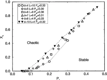
Fig. 1. Critical line separating stable and "chaotic" behaviour for Pat _close_to_{½, RA distribution, for different}

dimensions.

possibility to get a class 4 behaviour. From our simulations on the BSPHI model, the stable configurations, for d _> 2, are fixed points or period-two limit cycles, which also confirm the droplet-type arguments of Bennet et al [ 14], which limit the possible patterns of collective states in d _> 2 to be at most of period two. We shall recall that, despite the fact that the higher dimensions introduce a mean-field tendency (with the increase in the number of neighbours) that could lead the system to exhibit limit cycles of periods greater than two or quasiperiodic behaviour [ 15,16], in this case the relevant parameter P1 depends also on the dimension and will be defined equivalently in all dimensions. So, in contrast to the survival windows defined in the cellular automata introduced by Chatr-Manneville, where the window is fixed, this tendency does not exist in our case.

In order to study only the influence of the activation threshold we have kept the

activation interval (Pat) as close as possible to 1, since as shown below, this choice

guarantees that the size of the activation window will not influence the results obtained. We have performed simulations for RA distribution varying d from 2 to 10, using different values of L for each dimension considered. From Fig. 1, we see that the smaller the dimension the smaller PI*, as it should be since P1 depends on the number of different possibilities of B = 2 neighbours, which itself depends on the value (2d + 2). We also note that for d > 8 the critical curves seem to collapse into the same curve; without considering the first point (related to small P1) it can be approximated by a linear

growth of Xc with/'1. Going to higher dimensions, as Pl* increases the xc associated to

it also grows. In other words, going through higher dimensions the activation threshold becomes large in order to avoid the "chaotic" behaviour, and there is an enlargement of

(9)

x ~ 1.0

0.8

0.6

0.4

0.2

O P a t = 0 . 1 9 0 Pm = 0 . 2 5 [ ] Pat = 0.31 / k - A P ~ t = 0 . 3 8 I>P~t = 0 . 5 0 • P.t : 0 . 5 6

Chaotic

/ / / / /

, • r

0"00.0 ' ~"-0.1 0.2

P1

o f l l

/ / J

Stable

r

0.3 0.4

/ /

0.5

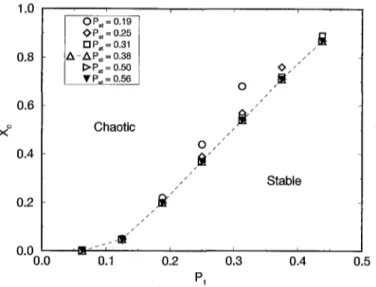
Fig. 2. Critical concentration (Xc) versus the activation threshold parameter (P1) for d = 7, L = 6 and RA

distlibution for different values of Pat.

In Fig. 2 we show the behaviour o f the critical line in the (P1, x) parameter space,

for d = 7, L = 6 and R A distribution for different values o f Pat. For Pat > 0.31, all

the critical lines collapse to the same line. I f the activation interval is too small, it will

influence the automaton behaviour. On the other hand, i f Pat >- 1 it does not influence

the dynamical evolution o f the system.

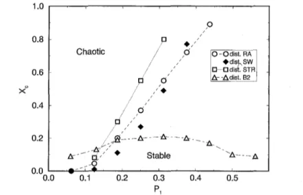
In order to investigate the influence o f the choice o f initial distribution on the behaviour o f the cellular automata, we have performed simulations for d = 7, L = 6 and Pat = 0.3125 using four different distributions: SW, RA, STR and B2. F r o m Fig. 3 we see very similar behaviour for both S W and R A distributions. The differences appear when P1 is small and when P1 is close to PI*. This is better shown in Fig. 4, where we present data concerning only the R A and S W distributions for d = 10, L = 4 and Pat = 0.3175. So, for the R A distribution the activation threshold necessary to avoid the stable-"chaotic" transition gets higher, but also the region o f stable configuration in the parameter space gets large. Other simulations were performed in order to better compare S W and R A distributions in all dimensions, from which we get that the S W curve (xc versus P1) crosses the R A one at the same point, as expected, since the P1 definition depends on d.

The STR distribution seems to not favour the "chaotic" behaviour (it enlarges the region o f stable configuration behaviour); its PI* is smaller than the m a x i m u m value Pl for the S W and R A distributions. This distribution seems to be m o r e natural than the other ones, since it takes into account two different probabilities ( x and y ) ; actually y is a r a n d o m number and the distribution is made based on the comparison between y and x.

(10)

1.0

x o 0.8

0.6

0.4

0.2

O - Odist. RA O d i s ~ S W

O--- 0 dist. STR

Z~- -Adist. B2

Chaotic

ah i O , I

0.1 0.2

J []

/:" /i ~

,,/ J i i J ,.:'

0 0 /

/:: j /

,:," J / / ,," / O /" J ~

Stable

i

0.3 P1

~ A - _ _ A

i F

0"00.0 0.4 0.5

Fig. 3. Critical concentration (Xc) versus activation threshold parameter (P1) for d = 7, L = 6 and Pat = 0.3125 for four different distributions: SW, RA, STR and B2.

1.0

x o 0.8 0.6 0.4 0.2 Chaotic o [] o 0.1 o [] o [] O

O dist. RA • dist. SW

o

Stable

I

0"00.0 0.2 0 3 0.4 0.5

Pl

Fig. 4. Critical concentration (xc) versus activation threshold parameter (P1) for d = 10, L = 4 and Pat = 0.3175 considering only SW and RA distributions.

(11)

1.0

0.8

0.6 x o

0.4

Stable

i r

4 6

d

Chaotic

0 . 2 i

2 8 10

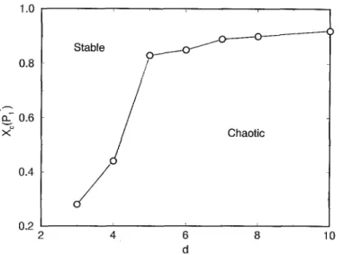
Fig. 5. Critical concentration Xc for the Pl* (the last value of P1 for which we still obtain the stable-"chaotic"

transition) for the different dimensions considered, considering the RA distribution and Pat close to ½.

a slight increase on the concentration will cause the system to attain the same situation as in case (a) because o f the large number o f B = 2 neighbours that will be available. The critical concentration xc varies inside a small range o f values, attaining a m a x i m u m

value around 0.20; for small and large P1, Xc is close to 0.1.

We have plotted xc (Px*) for different dimensions in Fig. 5, using the R A distribution and Pat ~ ½. As one can see, for low dimensions Xc grows fast, but for d > 5 the

variation is not very strong, actually it seems that Xc tends to an asymptotic value close

to one.

We have also p e r f o r m e d simulations in order to analyse the effect o f the finite size on the results. As expected, this effect are important only for small L in low dimensions but they are almost negligible in higher dimensions and for large L in low dimensions.

4. Conclusions

We have investigated the influence o f the random initial distribution o f a three state automata, used to m o d e l the i m m u n e repertoire, on its dynamical evolution. We have p e r f o r m e d simulations considering four different distributions. We got quite similar behaviour for three o f them - a well defined line separating the parameter space in two regions: one o f stable configurations (fixed point or limit cycles) and another one o f "chaotic" behaviour. A n o t h e r very distinct behaviour was obtained for the distribution that favour the number o f B = 2 neighbours, as expected, since the automaton rule depends on the number o f B = 2 sites in the neighbourhood.

(12)

automata, as it should be, since t h e window definition is based on the proliferation function. If the activation interval is too small it will influence the behaviour of the cellular automata, in the sense that it will enlarge the stable region in parameter space.

1

For Pat >- ~ the system seems to converge asymptoticaly to the same behaviour no matter the value of Pat.

A very interesting result obtained is the existence of the stable-"chaotic" transition, depending on the value of PI, for d _> 2, whereas earlier work found it only for d _> 4. We have also found a m a x i m u m value PI*, such that, for P1 _< Pl* this transition is always present and xc grows as Pa -+ PI*-. Above Pa* the transition disappears and the system always evolves to stable configurations.

F r o m the point of view of cellular automata we have obtained the phase diagrams mapping the range of parameters for which we attain distinct behaviour. Such diagrams are not easily found in the literature and enable us to define the critical region probably associated to a class 4 behaviour.

A c k n o w l e d g e m e n t s

This work was partially supported by CNPq, FINEP and CAPES. We would like to thank to D. Stauffer for the access to the original Fortran code used for their simulations. R M Z S thanks N. Caticha, O. Kinouchi and M. Copelli for the enlighting discussions. We also thank to S.L.A. de Queiroz and A.M.N. Chame for the critical reading of the manuscript.

R e f e r e n c e s

[ 1 ] A.S. Perelson, in: Theory and Control of Dynamical Systems, S. Andersson, ed. (World Scientific, Singapore); preprint Santa Fe Institute 92-01-002 (1992).

[2] H. Atlan and I.R. Cohen, eds., Theories of Immune Networks, Springer Series in Synergetics, Vol. 46 (Springer-Verlag, Berlin-Heidelberg, 1989).

[3] A.S. Perelson, ed., Theoretical Immunology, Parts I and II, Santa Fe Institute Studies in the Sciences of Complexity (Addison-Wesley, 1988).

[4] N.K. Jeme, Ann. Immunol. (Inst. Pasteur) C 125 (1974) 373-389. [5] D. Stauffer and G. Weisbuch, Physica A 180 (1992) 42-52.

[6] R.J. De Boer, L. Segel and A.S. Perelson, J. Theor. Biol. 155 (1992) 295-333. [7] A. Coutinho, Immunol. Rev. 110 (1989) 63-87.

[8] D. Holmberg, A. Andersson, L. Carlson and S. Forsgen, Immunol. Rev. 110 (1989) 89-103. [9] A.S. Perelson and G.E Oster, J. Theor. Biol. 81 (1979) 645.

[10] R~M. Zorzenon dos Santos, Physica A 196 (1993) 12-20.

[11] G. Weisbuch, R. De Boer and A.S. Perelson, J. Theor. Biol. 146 (1990) 483. [12] A.U. Neumann and G. Weisbuch, Bull. Math. Biol. 54 (1992) 21.

[ 13] S. Wolfram, in: Theory and Applications of Cellular Automata (World Scientific, 1986).

[ 14] C.H. Bennet, G. Grinstein, Y. He, C. Jayaprakash and D. Mukamel, Phys. Rev. A 41 (1990) 1932. [15] H. Chat6 and P. Manneville, Europyhys. Lett. 14 (1991) 409.