Partial obstruction of flow through a channel

(1)

Partial obstruction of flow through a channel

A.D. Araújo

a,

*

, Izael A. Lima

a

, M.P. Almeida

a

, J.B. Grotberg

b

, José S. Andrade Jr.

a a_{Departamento de Física, Universidade Federal do Ceará, Campus do Pici, 60451-970 Fortaleza, Ceará, Brazil}

b_{Department of Biomedical Engineering, University of Michigan, Michigan, MI 48109-2099, United States}

a r t i c l e i n f o

Article history:

Received 22 May 2017

Received in revised form 7 October 2017 Available online 21 November 2017

Keywords:

Fluid flow Drag force

Numerical simulation Reynolds number

a b s t r a c t

We study the disturbance on two-dimensional flow generated by a circular obstacle of radiusrplaced downwind in front of a duct of widthwat a distanceλbetween the center of the obstacle and the inlet position of the channel. Our results show that, at low Reynolds conditions, the fluxφat the duct exhibits distinct regimes for differentλintervals.

1. Introduction

The hydrodynamical interaction between a flowing fluid and suspended particles is an interesting problem with important applications in science and technology [1–3]. There are several situations where microscale suspended soft particles might clog the duct cross section disturbing or even interrupting the flow. When the fluid is viscous and the particles are deformable, they can readily undergo large deformations to accommodate the hydrodynamic forces. This process is observed in many situations and scales, from blood flow in microscopic vessels up to sewage flow in macroscopic pipes. In vasculatory systems, we find some extreme cases where the cross section of the capillary vessel and the size of the blood cells that flow through them have the same order of magnitude [4]. In this case, the cells must undergo a large deformation in order to travel along the vessels. In some blood diseases the deformability potential of the red cells is reduced [5,6] blocking the flow through microvascular vessels. In other cases the blood can coagulate to form large clusters that behave like a solid [7]. As a consequence of these processes, in the extreme limit, the fluid flow is eventually interrupted. It is therefore important to understand how the presence of an obstacle with the same dimension of the duct width disturbs the flow and changes the flux across this duct.

Due to the broad applicability of this problem, many approaches and techniques have been used to simulate the interaction between the fluid and particles. Some of them belong to a group of pseudo-particle methods that form a class of multi-scale simulation approaches in computational fluid mechanics. Among them, we have lattice-based cellular automata methods (lattice gas, lattice Boltzmann) [8] and off-lattice approaches (dissipative particle dynamics, direct simulation Monte Carlo, multiple particle collisions) [9–12]. Alternatively, one may solve the Navier–Stokes equation directly finding the pressure and velocity fields [13,14] and then introduces particles that can interact or not with the fluid.

The interaction of a particle with the fluid flow within a channel has several characteristic lengths which are related to the particle and channel geometrical dimensions [15]. A straightforward way to approach this problem, consists basically in solving the Navier–Stokes equation in the presence of particles for a set of boundary conditions, calculating the velocity and the pressure fields. Subsequently, the particles are moved by a very small distance, according to the drag forces exerted

*

Corresponding author.

(2)

2020 A.D. Araújo et al. / Physica A 492 (2018) 2019–2026

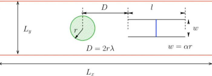
Fig. 1. Schematic view of the problem investigated here. Basically, the geometry consists of a box with lengthLxand widthLy. The channel has a length

land a tunable widthw=αr, whereαis a dimensionless parameter. The circle obstacle with radiusris located in front of the channel with its center distantD=2rλfrom the entrance, whereλis a dimensionless parameter.

on them, the velocity and pressure fields are calculated again, and so on. Using this numerical calculation sequence, we can determine how each particle interferes in the flow around its surface and force acting on it. Furthermore, we can apply this idea to study a traveling particle transported by a fluid approaching to a narrow channel.

The main purpose of this paper is to study how the flow disturbance caused by a solid obstacle inside a duct influences the flux through a channel placed downwind the obstacle as a function of the distance between the obstacle and the channel entrance. We measure the flux

φ

through a channel placed a distance

λ

downwind the obstacle. For this, we numerically solve the Navier–Stokes equation to compute the flux

φ

and the drag force over the obstacle as a function of

λ

. Our results indicate the occurrence of distinct flow regimes for different values of

λ

, with the flux

φ

decaying as a power-law in the limit

λ

→

0. Finally, the presence of a minimum in the drag force over the particle is also observed for a given

λ

value.

2. Model

We study the system shown inFig. 1that consists of a two-dimensional duct with lengthLx

=

100 m and widthLy

=

20 m,

inside which there is a smaller channel of lengthland width

w

with its longitudinal axis aligned along the axis of the enclosing duct. A circular solid obstacle with radiusr

=

1 m is placed at a distanceDupwind the entrance of the smaller channel with its center on the duct’s axis. The various geometric configurations we use are described in terms of two non-dimensional parameters, namely,

λ

=

D

/

(2r) and

α

=

w/

r, with

α >

0

.

5 for all simulations presented. In order to avoid border effect, the width of the ductLyis at least one order of magnitude larger than the channel width w. We impose no-slip boundary

conditions along the entire solid–fluid interface. At the inlet (x

=

0), we impose the conditions,ux(0

,

y)

=

Vanduy(0

,

y)

=

0,

while the boundary condition at the outlet (x

=

Ly) is imposed to be

∇

p

=

0. The Reynolds number is defined asRe

=

ρ

Vr

/µ

,

where

ρ

and

µ

are, respectively, the density and the viscosity of the fluid, andVis the velocity at the inlet section. We take

ρ

=

1 kg

/

m3_and

_µ

₌

_{1 kg}

_/

_{(m s).}

We use the CFD software Fluent (Ansys, Inc.) [16] to numerically compute the steady-state solution of the two-dimensional flow of an incompressible Newtonian fluid in terms of the Navier–Stokes and continuity equations,

ρ

u

⃗

· ∇ ⃗

u

= −∇

p

+

µ

∇

2_u

_⃗

₍₁₎

∇ · ⃗

u

=

0 (2)

whereu

⃗

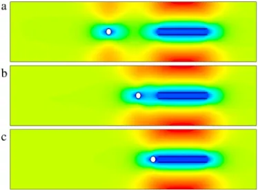
is the velocity andpthe pressure.

InFig. 2we show a typical velocity field obtained from numerical simulations in a regime of low Reynolds number,

Re

=

0

.

356, for three different values of

λ

and fixed width

w

. The colors ranging from blue to red correspond to low and high velocity magnitudes, respectively. The contour plot of the velocity magnitude clearly reveals that, as the obstacle is approaching the channel entrance, the wake region of the obstacle, shown as the dark region behind it, reaches the channel and the obstacle begin to play a more significant role on the flow towards the channel.

3. Results and discussion

In order to quantify the obstacle influence on the channel flux, we calculate the flux

φ

through the channel, as the integral of the velocity along the linear distance orthogonal to the flow times the length of this line. In our analysis we have normalized the flux

φ

by the total flux

φ

0calculated as the same of the flux

φ

but now considering the entrance of the duct. In that case,

φ

0is the total flux getting inside the duct while

φ

is the fraction of this flux that goes inside the inner channel.Fig. 3shows a log-linear plot of the normalized flux (

φ/φ

0) as a function of

λ

, for five different values of

w

. Three distinct regimes of

φ/φ

0can be clearly identified. In the limit of large

λ

(

λ

≥

10), the flux

φ

tends to a saturation value

φ

s

which depends on the width

w

as a power law,

φ

s

∝

w

2.66, as the collapse of all curves in this region indicates (see the inset

(3)

Fig. 2. Velocity fields calculated for three values ofλandwequal to the obstacle diameter. Fluid is pushed from left to right at low Reynolds conditions (Re=0.356). The colors ranging from blue to red correspond to low and high velocity magnitudes, respectively. In (a) we haveλ=10, (b)λ=4 and (c)

λ=1.0. Asλdecreases the obstacle’s wake region reaches the entrance of the channel. (For interpretation of the references to color in this figure legend, the reader is referred to the web version of this article.)

Fig. 3. (Main panel) Semilog plot showing the normalized flux across the channel as a function ofλ=D/2r, whereDis the distance from the center of the obstacle to the channel entrance andris the obstacle radius. These results correspond toRe=0.356, and the symbols refer to different values of the channel width: (⃝)α=1.0, (□)α=1.25, (⋄)α=1.5, (△)α=1.75, (◁)α=2.0. The inset at the bottom shows the log–log plot of saturated fluxφsas a function ofw. The solid line corresponds to the least-squares fit of the data to a power law,φs∼wβ_{, with the scaling exponent}_β₌₂_.₆₆_±₀_._{01. The inset}

at the top shows the rescaling of the normalized flux as a function ofλ.

The second regime is a logarithmic behavior in the interval 1

≤

λ

≤

10 which is independent of

α

, since as we rescale the normalized fluxes curves by the appropriated value

β

, they collapse in the same one. Finally, the third region corresponds to the interval

λ

c(

w

)

< λ <

0

.

1, where

λ

c

=

λ

c(

w

) is a lower bound value defined as

λ

c(

w

)

=

{

0

.

25

√

4

−

α

2

_{, α >}

₀

_.

₅

0

,

α

≤

0

.

5

.

(3)

This is the smallest possible value of

λ

, which represents the closest position that the obstacle can get to the initial cross-section of the channel. When the obstacle touches the channel’s walls the flux is null. As shown inFig. 4, the dependence on

λ

of the normalized flux

φ/φ

0in this critical regime can be well described in terms of a power-law,

φ

0

(4)

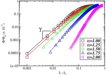
Fig. 4.The log–log plot of the normalized fluxφ/φ0as a function of (λ−λc). The solid lines are the least-square fits to the data sets in the scaling regions of a power-law, with exponentsγ=1.76±0.03,γ=1.79±0.08,γ=1.86±0.09,γ=2.22±0.05,γ=3.26±0.02 correspond toα=1.0,α=1.25,

α=1.5,α=1.75 andα=2.0, respectively.

Fig. 5. Plot in a log-linear scale of the flux across the channel versus the distanceλ. The symbols correspond to different Reynolds numbers, namely, (squares)Re=0.3556, (circles)Re=3.356, (triangles up )Re=24.00 and (triangles left )Re=35.56. The width of the channel correspond to the case whereα=1.

with exponent values

γ

=

1

.

76

±

0

.

03

,

1

.

79

±

0

.

08

,

1

.

86

±

0

.

09

,

2

.

22

±

0

.

05 and 3

.

26

±

0

.

02 corresponding to

α

=

1

.

0

,

1

.

25

,

1

.

5

,

1

.

75 and 2.00, respectively. These results indicate that, the smaller is the ratio

w/

rslower is the way that the flux increases with

λ

.

Next we investigate the effects ofReon the flux inside the inner channel. Here we modify the Reynolds number only changing the velocity magnitudeVat the inlet of the larger channel for a fixed value

α

=

1

.

0. As we can see inFig. 5, the normalized flux

φ/φ

0has maintain the same behavior as a function of the Reynolds number, with the presence of three characteristic regimes as discussed before. The only notable effect is the displacement of the crossover region, from the saturation to logarithmic regime, in the direction of higher values of

λ

as the Reynolds number increases. For high Reynolds number the presence of the obstacle has an influence in the flux at greater distance from the channel, when we compare with the same condition for

α

=

1

.

0 and lowerRe.

It is interesting to investigate how the drag force on the obstacle is influenced by the geometrical setup of the flowing system. Essentially, the drag forceFddepends substantially on the boundary layer configuration and viscosity. In our system,

the fluid flowing in the immediate vicinity of the obstacle’s surface changes as the obstacle is getting close to the entrance of the small channel. Here the drag forceFdis calculated as,

Fd

=

∫

S

(5)

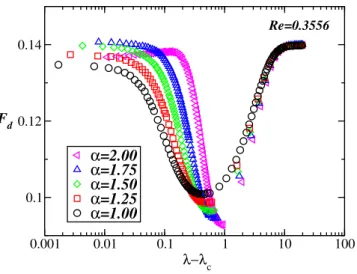
Fig. 6.The Log-linear plot of the drag force over the obstacle as a function of (λ−λc) for different values ofw. The Reynolds number isRe=0.3556.

whereF

⃗

p and

⃗

Fvare the pressure and viscous forces, respectively. The integral is taken over the entire surfaceS of the

obstacle.

As shown inFig. 6,Fdpresents a minimum for certain values of

λ

. Moreover, we observe that the minimal drag force

decreases with

α

, while its corresponding

λ

value increases. These minimal values, for all

w

, are surrounded by two plateaus localized at the regions of small and large

λ

. The drag force shows a symmetry around the minimal, however at the region of plateaus the drag force presents a small deviation for the saturation value. For large

λ

, the drag force presents the same saturation value as a function of

α

, whereas for small distance the drag force exhibits a slight difference on the plateau that depends on

α

. When we compare the value of the drag force for larger values of

λ

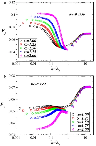
calculated here with the one from the analytical expression [17], considering the flux around a cylinder, the difference between those values is lower than one order of magnitude.

In order to investigate, which term has a major contribution in the drag force we analyze the independent contributions of the pressure and viscous forces on the drag. We plot inFig. 7a and7b the pressure and the viscous forces respectively, over the obstacle for a set of values of the distance (

λ

−

λ

c), for different values of

α

. For large values of

λ

, the drag force receives

the same contribution from both terms however, for small values the major contribution comes from the pressure force term. The pressure force presents a well defined minimum in terms of the distance

λ

−

λ

c, which is around

λ

−

λ

c

≈

0

.

8,

which changes only slightly with

α

. Now considering the effect over the viscous forceFv, as

λ

decreases the viscous force

presents a local minimum followed by a little bump and then slowly decay. Note that both, pressure and viscous forces present a minimum value at the region of intermediate values of (

λ

−

λ

c), which reinforces the presence of a minimum at

the same region of (

λ

−

λ

c) in the drag force. To emphasize the behavior of the drag force in the direction of its minimal

value, we chose one particular case, namely,

α

=

1

.

0 and performed additional simulations considering a very refined set of

λ

values. The result is plotted inFig. 8. As shown, the drag force has a smooth behavior around its minimum. Similar results (not shown) were obtained for the other values of

α

.

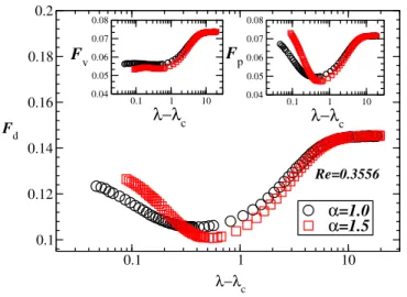
There is a suspicion that the presence of the minimum in the drag force could be an artifact from the symmetry condition of the problem. Then we do a further analysis for a no symmetric case. We show inFig. 9that a minimal drag force can also be observed if the obstacle is shifted from the symmetry line (in they-direction) by a distance corresponding to 20% of its radius. Furthermore, as shown in the inset ofFig. 9, the forcesFdandFvfollow the same qualitative behavior as a function

of the distance

λ

with respect to the non-shifted case. However, the values of

λ

for which the drag becomes minimum are different. Shown inFig. 10is the dependence of the lift on the shifted obstacle with

λ

for different values of

α

. The way the lift increases and the maximum value do not depend on the channel width

α

, but the way it decreases after this maximum until reaching a negative value is slightly dependent on

α

. Since the lift is a force perpendicular to the oncoming flow direction, then its negative values only means a change in direction of the applied force. In our case, the lift pushes the obstacle towards the symmetry line trying to restore the equilibrium position. As the distance

λ

keep decreasing, at a certain value of the distance

λ

, the lift has a sudden drop, which again depends on

α

, followed by a slowly decreases at the point where the obstacle is almost connected to the channel entrance. This interesting behavior confirms the fact that when the obstacle is out of symmetry line the flowing fluid surrounding the obstacle pushes it to retrieve the original (symmetric) position.

(6)

Fig. 7.Log-linear plot of the contribution of each term to the drag force over the obstacle as a function of (λ−λc) for a set of representatives values ofα. In (a) we have the pressure force contribution and in (b) the viscous force contribution. The sum over these two terms gives the total contribution of the drag forceFdaccording to Eq.(5). Symbols correspond to the following values ofα; (⃝)α=1.0, (□)α=1.25, (⋄)α=1.5, (△)α=1.75, (◁)α=2.0 .

The Reynolds number isRe=0.3556.

obstacle in front of the channel creates a narrow region where the drag force has a minimal value. If an obstacle is placed in a moving fluid close to a channel entrance, it should be transported at a lower speed compared with other regions. Furthermore, thinking in terms of a elastic obstacles, at this particular region the obstacle should deform less than in other regions.

4. Conclusions

In summary, we have investigated how the flux inside a channel is affected by the presence of an obstacle located upwind of the channel’s entrance. The flux across the channel shows three different behaviors as the distance

λ

between the channel and the obstacle changes. Furthermore, the smaller is the ratio (

w/

r), represented here by

α

, the slower is the flux variation with

λ

. The effect of increasing the Reynolds number was also investigated and our calculations confirm that the presence of the obstacle affects the fluxΦat longer distances for high Reynolds number. In addition, the drag force calculated over the obstacle has a minimum value for a certain value of

λ

which depends on

α

. By shifting the obstacle in they-direction from the center line in thex-direction, no qualitative changes could be observed in the overall behavior of the drag force, namely, it still exhibits a minimum for an intermediate value of

λ

.

(7)

Fig. 8. Log-linear plot of the drag force and the contribution of each term over the obstacle as a function of (λ−λc) calculated for a very refined set ofλ

values around the minimum region. Symbols correspond to the following (⃝) drag force, (□) pressure force and (△) viscous force. The Reynolds number is

Re=0.3556 andα=1.0.

Fig. 9.Log-linear plot of the drag force versus (λ−λc) for the shifted obstacle case. In the main plot we have the total drag force while the two insets we show the viscous force (left) and pressure force (right). In all sets, symbols correspond to: (black⃝)α=1.0, (red□)α=1.5. The Reynolds number is 0.3556. The minimal distance before the obstacle reaches the channel entrance is lower than the minimal distance in the symmetrical case. The off-symmetrical case also confirms the presence of a minimal behavior in the drag force. (For interpretation of the references to color in this figure legend, the reader is referred to the web version of this article.)

where the minimal drag force happens, the cell should undergo the minimum deformation in its shape which has an important effect over the flow resistance [18]. It is hoped that the results of this study will help guiding future experimental works on the fluid–particle interaction in the neighborhood of a channel entrance at level of micro-scale environments.

Acknowledgments

(8)

Fig. 10.The Log-linear plot of the lift as a function of (λ−λc) in the case of the shifted obstacle. The Reynolds number is 0.3556 and the channel width are

α=1.0 andα=1.5. The dashed line highlight the zero value of the lift.

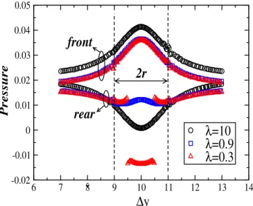
Fig. 11. The pressure profile calculated along two lines in front of the obstacle and behind the obstacle for different distancesλ. The channel width is

α=1.0 andRe=0.3556. The discontinuity in the pressure calculated behind the obstacle forλ=0.3 correspond to the part of the obstacle that is already inside the small channel. The two dashed lines correspond to the border limits of the circular obstacle.

References

[1]S.C. Kohale, R. Khare, J. Chem. Phys. 129 (2010) 234706.

[2]A. Ambari, B. Gauthier-Manuel, E. Guyon, J. Fluid Mech. 149 (1984) 235. [3]S. Ryu, P. Matsudaira, Chem. Eng. Sci. 65 (2010) 4913.

[4]Y.C. Fung, Biomechanics: Circulation, Springer-Verlag, 1996.

[5]Y.C. Fung, Biomechanics: Mechanical Properties of Living Tissues, Springer-Verlag, 1981. [6]K. Tsukada, E. Sekizuka, C. Oshio, H. Minamitani, Microvasc. Res. 61 (2001) 231. [7]R. Fahraeus, Phys. Rev. 9 (1929) 241.

[8]D.H. Rothman, S. Zaleski, Lattice-Gas Cellular Automata: Simple Models of Complex Hydrodynamics, Cambridge University Press, 1997. [9]P.J. Hoogerbrugge, J.M.V.A. Koelman, Europhys. Lett. 19 (1992) 155.

[10]P. Español, P. Warren, Europhys. Lett. 30 (1995) 4423. [11]R.D. Groot, P.B. Warren, J. Chem. Phys. 107 (1997) 4423. [12]A. Malevanets, R. Kapral, J. Chem. Phys. 110 (1999) 8605.

[13]A.D. Araujo, J.S. Andrade, H.J. Herrmann, Phys. Rev. Lett. 97 (2006) 138001. [14]A.D. Araujo, W.B. Bastos, J.S. Andrade, H.J. Herrmann, Phys. Rev. E 74 (2006) 010401. [15]D.J. Tritton, Physical Fluid Dynamics, Oxford University Press, 1988.

[16] ANSYS, Inc. Southpointe 2600 ANSYS Drive Canonsburg, PA 15317 USA.