*
Revista Brasileira de Ensino de F´ısica,v. 33, n. 2, 2701 (2011) www.sbfisica.org.br
Notas e Discuss˜oes
Gauss’s law, infinite homogenous charge distributions
and Helmholtz theorem
(A lei de Gauss, distribui¸c˜oes de carga homogˆeneas de extens˜ao infinita e o teorema de Helmholtz)
A.C. Tort
1Instituto de F´ısica, Universidade Federal do Rio de Janeiro, Rio de Janeiro, RJ, Brazil
Recebido em 3/1/2011; Aceito em 23/2/2011; Publicado em 3/6/2011
Rediscutimos a validade da lei de Gauss no caso de distribui¸c˜oes discretas e cont´ınuas de carga que se esten-dem por todo o espa¸co.
Palavras-chave: eletromagnetismo cl´assico, eletrost´atica, lei de Gauss.
We rediscuss the validity of Gauss’s law in the case of homogenous discrete and continuous charge distribu-tions fulfilling all space.
Keywords: classical electromagnetism, electrostatics, Gauss’s law.
In physics, some questions that we can formulate though frequently not realizable from a practical point of view, must as a matter of principle be satisfactorily answered. Moreover, they can be pedagogical useful tools and help the teacher to introduce new topics or discuss particularly hard ones. The following interest-ing question belongs to this type of question and can be found in [1]: Given a uniform charge distribution
ρ that fulfills all the space, what is the value of the electric field at an arbitrary point of the distribution? The answer given in [1] though correct is nevertheless intriguing. By symmetry the electric field must be zero everywhere which makes perfect sense, but this means that the electric flux through an arbitrary surface S enclosing a certain charge Q(S) is zero in conflict with the integral form of the Gauss’s law that states that the flux must be equal to Q(S)/ǫ0. In order to keep the symmetrical solution for the field it is stated that Gauss’s law is not valid in this situation because there are charges at the infinity. It is pedagogically worth to understand and rediscuss this problem and its answer and this is our aim in what follows.
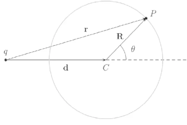
Let us begin by taking an alternative route to Gauss’s law. Consider a point charge q placed at a distancedfrom a pointCand a hypothetical Gaussian sphere of radiusR centered atC, see Fig. 1. Consider also a point P on the surface of the Gaussian sphere. If the distance of the point charge to P is r, then the electric field at P is given by
Figure 1 - Point charge and hypothetical Gaussian spherical sur-face.
E= q
4πǫ0r2
ˆer. (1)
It is convenient to treat d, R, and r as vectors, then r=d+Rand we can write
ˆ er=
r
r =
d+R
r =
d+R
(d2+R2+ 2dRcosθ)1/2, (2) whereθplays the role of a polar angle. The electric flux through an infinitesimal area centered aroundPis given bydΦ =E·nˆda, where the outward normal vectornˆat
Pcan be set equal toˆeR=R/R. Therefore, the electric
flux through the infinitesimal areada=R2sin θ dθ dϕ is
1
E-mail: [email protected]; [email protected].
2701-2 Tort
dΦ = q
4πǫ0
(d+R)·ˆeRda
(d2+R2+ 2dR cosθ)3/2
= q
4πǫ0
(dcosθ+R)R2 sinθ dθ dϕ (d2+R2+ 2dRcosθ)3/2 . (3) The total flux through the spherical surface is
Φ = qR
2d
2ǫ0
Z π
0
cosθsinθ dθ
(d2+R2+ 2dRcosθ)3/2
+ qR
3
2ǫ0
Z π
0
sinθ dθ
(d2+R2+ 2dR cosθ)3/2. (4) Introducing the standard variable transformationx = cosθ and the real positive parameter λ = d/R, the total flux can be recast into the form
Φ (λ) = q
2ǫ0F(λ), 0≤λ <∞, (5) whereF(λ) is defined by
F(λ) =λ Z +1
−1
x dx
(1 +λ2+ 2λx)3/2+
Z +1
−1
dx
(1 +λ2+ 2λx)3/2. (6) This integral can be evaluated and the result is
F(λ) = 1−signum (λ−1), (7) where for a real numberp
signum (p) =
½
+1, ifp >0,
−1, ifp <0. (8)
It folows that ifd > R, that isλ >1, then F(λ) = 0, and ifd < Ror 0≤λ <1, thenF(λ) = 2. Ifd=R, or
λ= 1, the integral is undefined. Therefore we conclude that ifq is outside the Gaussian spherical surface, the electric flux is zero, ifqis inside the flux is equal toq/ǫ0. Because there is nothing special about the direction we have chosen in Fig. 1 to evaluate the flux we can extend this result to an arbitrary number of point charges. If we have N point charges outside the Gaussian sphere and M point charges inside of it we can make use of the superposition principle and write for the total flux
Φ = 1
ǫ0
N+M
X
j=1
qjF(λj), (9)
where λj =dj/R. Making use of Eq. (8), we see that
Eq. (9) simplifies to
Φ = 1
ǫ0
M
X
j=1
qj. (10)
All charges outside the region enclosed by Gaussian sur-face, no matter where they are, do not contribute to the
electric flux through the Gaussian sphere. This result can be easily extend to continuous charge distributions. Of course we can obtain Gauss’s law by making use of the concept of solid angle and arbitrarily shaped sur-faces, but our Gaussian sphere can be made as large as we please and enclose any number of point charges (or a portion of the continuous distribution).
The main lesson that we can infer from the calcu-lation above is that having charges at the infinity is not a good reason to discard Gauss’s law in the context posed in [1], because these charges do not contribute to the flux whatsoever and hence seem not to be respon-sible for the failure of Gauss’s law in this context. The flux depends entirely on the charges inside the Gaussian sphere and we still have a conundrum to solve.
One way out of it is to consider Maxwell’s two equa-tions for electrostatics
∇ ·E= ρ
ǫ0
, (11)
and
∇ ×E= 0, (12)
and realize that the first one is not compatible with the answer dictated by the underlying symmetry of the distribution, that is, E = 0 everywhere is not a valid solution of Maxwell’s equations when we take ρ as a continuous uniform charge distribution fulfilling all the space. This solution is somewhat frustrating but seems to be the correct one. Is there some other solution for the electric field whenρis a continuous uniform charge distribution fulfilling all the space? Yes, but there is a price we must pay, the homogeneity of the space is lost. The solution is
E(r) = ρ 3ǫ0
(xˆx+yyˆ+zˆz) = ρ 3ǫ0
r. (13) Isotropy is retained, but now there is a privileged point, the center of the distribution. Notice that given the na-ture of the charge distribution there are charges at the infinity (and the field increases indefinitely there). This solution is a mathematically valid solution of Eqs. (11) and (12) though it poses other kind of problems.
Gauss’s law, infinite homogenous charge distributions and Helmholtz theorem 2701-3
We can ask ourselves under what conditions Eqs. (11) and (12) and their gravitational analogues have a finite, physical meaningful solution, in other words, un-der what conditions a vector field F is determined by its divergence and its curl? This question makes sense if we also specify certain conditions that the field must obey on the boundaries of the region of interest, the boundary conditions. If we impose the condition that the vector field must vanish very far away from its finite, localized sources, Helmholtz’ theorem [3] assure us that the field is uniquely determined by its divergence and its curl. Specifically, given a vector field F(x), defined in some regionR, and the field equations
∇ ·F(x) =D(x), (14) ∇ ×F(x) =C(x), (15) with ∇ ·C(x) = 0, we can split F(x) into two parts, an irrotational part F1(x) such that ∇ ·F1 = D and ∇ ×F1 = 0, and a divergenceless oneF2(x) such that ∇ ·F2= 0 and ∇ ×F2=C. Then we can write
F1(x) =−∇Φ, (16)
and
F2(x) =−∇ ×A(x), (17) where Φ and Aare auxiliary functions defined inR. If we choose R conveniently and assume that the auxil-iary functions behave at least as 1/rvery far away from a field point labeled byx, make use of Green’s theorem, and finally perform the translationx→x−x′, we
ar-rive at
Φ(x) = 1 4π
Z D(x′)d3x′
kx−x′k , (18)
and
A(x) = 1 4π
Z C(x′)d3x′
kx−x′k . (19)
For more mathematical details and insights see [3–7]. This result is true for an extended localized source. For a pointlike source some extra care must be taken [3].
There are other examples of the trouble we can get into if we take too seriously unphysical situations and disregard appropriate boundary conditions. Consider,
for instance, a uniform but otherwise time-varying mag-netic field pervading all space. Because there is not a single point that we can consider as the center, sym-metry arguments lead us to conclude that the induced electric fields are null everywhere in conflict with Fara-day’s law.
The infinite homogeneous distributions that moti-vated this note do not obey the conditions under which Helmholtz’ theorem holds. But how we should deal with these types of distributions that appear also in the form of plane charge and mass distributions, infi-nite line distributions, etc.? First of all notice that they are unphysical, though usefulapproximations if certain conditions are met. For those cases, symmetry argu-ments and not Eqs. (11) and (12) or their gravitational equivalents can be used to determine the electrostatic or gravitational field just as Newton and reference [1] did though their answers are not valid solutions of the corresponding field equations.
Acknowledgments
The author is grateful to the referee for his/her careful reading of the original manuscript and pertinent sug-gestions.
References
[1] J.M. Levy-LeBlond and A. Botuli, La Physique en Questions Tome 2: Electricit´e et Magnetisme(Vuibert, Paris, 1999), 2nd
ed. Vers˜ao em portuguˆes,A Electrici-dade e o Magnetismo em Perguntas (Gradiva, Lisboa, 1991).
[2] E. Harrison, Cosmology: The Science of the Universe
(CUP, Cambridge, 2000), 2nd
ed.
[3] R. Becker, Electromagnetic Fields and Interactions
(Dover, New York, 1982).
[4] D.J. Griffiths,Introduction to Electrodynamics (Pren-tice Hall, Upper Saddle River, 1999), 3th
ed.
[5] W.K.H. Panofsky and M. Philips,Classical Electricity and Magnetism(Addison-Wesley, Reading, 1962), 2nd
ed.
[6] G.B. Arfken and H.J. Weber,Mathematical Method for Physicists (Academic, San Diego, 1995), 4th
ed. [7] H. Fleming, Revista Brasileira de Ensino de F´ısica 2,