Interpretation of ionospheric F-region structures in the vicinity of
ionisation troughs observed by satellite radio tomography
G. A. Aladjev, O. V. Evstafiev, V. S. Mingalev, G. I. Mingaleva, E. D. Tereshchenko, and B. Z. Khudukon
Polar Geophysical Institute of the Kola Science Centre, Russian Academy of Sciences, Khalturina 15, 183010, Murmansk, Russia
Received: 31 March 2000 – Revised: 11 October 2000 – Accepted: 18 October 2000
Abstract. Tomographic images of the spatial distribution of electron density in the ionospheric F-region are pre-sented from the Russian-American Tomography Experiment (RATE) in November 1993 as well as from campaigns car-ried out in northern Scandinavia in November 1995 and in Russia in April 1990. The reconstructions selected display the ionisation troughs above the tomographic chains of re-ceivers during geomagnetically quiet and disturbed periods. Two mathematical models of the high-latitude ionosphere de-veloped in the Polar Geophysical Institute have been applied for interpretation of the observed tomographic images.
Key words. Ionosphere (electric fields and currents; ion chemistry and composition; plasma convection)
1 Introduction
The ionospheric ionisation trough is one of the most out-standing features of the subauroral ionosphere. It appears within a longitudinally elongated narrow strip equatorwards of the auroral zone. The main feature of the trough is that its electron density in the F-region is much lower than in the neighbouring regions (e.g. Moffett and Quegan, 1983). The trough is a quite steady ionospheric formation existing mainly in winter on the night-side of the Earth. Several meth-ods have been used in determining the distribution of the ionospheric plasma density in the vicinity of the trough.
The satellite radio tomography providing images of iono-spheric electron density has been successfully used in the Po-lar Geophysical Institute during the last decade. Its experi-mental set-up is to have a chain of ground-based receivers which carry out difference Doppler measurements using sig-nals from Russian navigational satellites flying close to 1000 km altitude and passing the chain. In tomographic measure-ments the observations consist of the phase difference of
co-Correspondence to:B. Z. Khudukon ([email protected])
herent radio waves at frequencies 150 and 400 MHz, which is proportional to the integral of the electron density (TEC, the total electron content) along the ray from the satellite to the receiver. Therefore, when the observations are made con-tinuously at a number of sites in the chain on the ground level while a satellite is flying along the chain, the integrals can be determined along the great number of rays crossing each other in the ionosphere. This means that the experi-ment is suitable for calculating the electron density in the vertical plane by means of tomographic inversion (Austen et al., 1986, 1988; Raymund et al., 1990; Andreeva et al., 1992). Several satellite tomography campaigns have been arranged by means of the PGI measuring equipment both in Russia, Scandinavia and in the USA/Canada (Kunitsyn et al., 1990, 1994, 1995; Foster et al., 1994; Markkanen et al., 1995). Many of the reconstructed images of the iono-spheric plasma contain well indicated troughs. The data anal-ysis shows quite interesting features of the trough behaviour. It is not easy to discover the physical reasons which cause the complicated behaviour of the ionospheric plasma in the vicinity of the trough region. However, a solution to this problem could help greatly in understanding some topics in ionospheric physics and, in particular, in understanding the factors which produce the trough formation. More than a dozen different mechanisms have been applied to understand the origin of the trough (Moffett and Quegan, 1983). How-ever, trough formation during different geophysical condi-tions is not yet understood so that the problem is still actual (Rodger et al., 1992).
2 Interpretation of tomographic measurements by means of a two dimensional mathematical model
It has been mentioned already that the trough is longitudi-nally elongated so that longitudinal changes of electron den-sity within the trough are much weaker than latitudinal vari-ations. Therefore the longitudinal variation of electron den-sity is neglected here, and a two-dimensional non-stationary model is used. The spatial variables in the model are altitude and distance in meridional direction.
2.1 Formulation of the model
We apply a multicomponent non-stationary model of the high-latitude ionosphere by Aladjev and Mingalev (1986), which allows the calculation of the ionospheric composition from 100 to 580 km. The model produces two-dimensional distributions of ionospheric constituents in the magnetic meridional plane. This plane is fixed in the Sun-Earth frame of reference, e.g. in coordinates of the magnetic latitude and magnetic local time (MLT). Two-dimensional distributions of ionospheric quantities are obtained by solving the appro-priate system of transport equations for the ions O+, O+2, NO+, N+2, and H+. This system consists of the continuity equations, simplified equations of motion and simplified en-ergy equations for the ions. In Cartesian coordinates with the
x-axis pointing horizontally along the magnetic meridian to-wards the equator and thez-axis pointing towards the zenith, the system of transport equations for ions of typei can be written as
∂Ni ∂t +
∂ ∂x NiV
x i
+ ∂ ∂z NiV
z i
=Qi−Li , (1)
g− 1 miNi∇
(NikTi)+ ei mi
(E+Vi ×B)=
X
n
1
τin(Vi −Vn) , (2)
X
n
miNi mi+mn
1
τin
h
3k (Tn−Ti)+mn(Vn−Vi)2
i
=0, (3)
whereNi,Vi =(Vix,Viy,Viz), andTi are the number density,
drift velocity, and temperature of ions of typei;Qi andLi
are the production and loss rates of ions of typei;mi andei
are their mass and charge;gis the gravity acceleration;kis the Boltzmann constant; 1/τinis the collision frequency
be-tween ions of typeiand neutral particles of typen, andVn, Tn, andmnare the velocity, temperature, and mass of neutral
particles of typen, respectively.EandBare the electric and magnetic fields. In Eqs. (2) and (3), the summation runs over all types of neutral particles included in the model, namely, O, O2, NO, N, N2, H, N(2D). The electron concentrationNe
is obtained from the condition that the ionosphere is electri-cally neutral, i.e:
Ne=
5
X
i=1
Ni .
More complete details of the model, such as the ionisa-tion process, the chemistry of positive ions, the numeri-cal method, the boundary conditions, the input parameters etc. are presented by Aladjev and Mingalev (1986), Aladjev (1989), and Mingalev and Aladjev (1983).
2.2 Trough formation during a daytime geomagnetically quiet period
Most of the trough measurements have been carried out during night-time hours by means of different observa-tional methods (Moffett and Quegan, 1983; Rodger et al., 1992). The tomographic observations made in Scandi-navia in November 1995 are different since they also con-tain images of clear daytime troughs. In this campaign a chain of four receivers extending from northern Norway to southern Finland was installed along a magnetic meridian. The receiver sites from north to south are Troms¨o (69.662◦ N, 18.940◦ E), Esrange (67.877◦ N, 21.064◦ E), Kokkola (63.837◦N, 23.058◦E) and K¨ark¨ol¨a (60.584◦N, 23.985◦E). These stations lie nearly on the same line which almost coin-cides with a magnetic meridian (see the map in Markkanen et al., 1995). The length of the chain is 1036 km and the site separations are 214, 458 and 364 km from north to south. Difference Doppler measurements were carried out in the ex-periment using signals from Russian navigational satellites, which fly at 1000 km altitude closely parallel to the receiver chain during their southward passages. They transmit coher-ent waves at 150 and 400 MHz frequencies applicable for difference Doppler measurements on the ground. Only pas-sages where the satellite path is not too far away from the receiver chain were selected for the analysis.
These data were then applied in tomographic inversion for calculating the F-region electron densities in the vertical plane along the satellite path. The inversion algorithm used in the tomographic analysis is based on the stochastic method and it is described by Markkanen et al. (1995). In the analy-sis, a grid is defined on the vertical plane above the receiver chain, and the inversion results are the electron densities at the grid points. Due to the curvature of the Earth, the grid elements have annular rather than rectangular shapes. The horizontal mesh size was 30 km on the ground level in the regions which will be shown in the figures. The vertical el-ement size was 25 km within 100–700 km height range, and 33.3 km elsewhere.
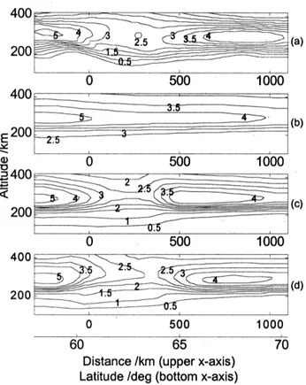
A contour pattern of the daytime F-region electron density in northern Scandinavia obtained from a satellite pass start-ing at 10:12 UT on November 17, 1995 is portrayed in the top panel of Fig. 1. The upperx-axis shows the horizon-tal distance on the ground (in km) from the most southern station (K¨ark¨ol¨a). The bottomx-axis represents geographic latitudeϕ. It can be seen that the horizontal size of the trough is of the order of 500 km.
Fig. 1. Contour patterns of the daytime electron density (×1011 m−3) observed in the vertical plane over the chain of receivers in Scandinavia at 10:12 UT on 17 November 1995.(a)Experimental reconstructed image obtained by means of stochastic tomographic inversion.(b)Model pattern obtained by excluding the electric field and particle precipitation.(c)Model pattern obtained by including an inhomogeneous meridional electric field but no particle precipi-tation.(d)Model pattern obtained by including both an inhomoge-neous electric field and precipitation of soft electrons.
same time sector, reported by Pryse et al. (1998) have their deepest zones near 75◦-latitude. Hence, unlike either the mid-latitude trough or daytime high-latitude trough, it occurs at different latitudes. This seems to be the main feature of the trough in Fig. 1a.
The next feature of the F-layer density Ne is that the alti-tudes of the layer maximum near the equatorial boundary of the region appear to be essentially higher than in the nothern-most part. Theoretically, the altitude of the F-layer maximum versus latitude is expected to behave just in an opposite way since the daytime spatial behaviour of the electron density is mainly defined by the solar ultraviolet radiation (Ivanov-Kholodny and Nikolsky, 1969). This fact indicates that the formation of the electron density distribution in the top panel of Fig. 1 is due to some other physical processes related not only to the solar ultraviolet radiation.
An attempt was made to perform a numerical simulation of the electron density distribution shown in Fig. 1a by means of the mathematical model formulated above. Some of the input parameters (date, time, solar and geomagnetic indices) were taken to match the conditions at the time of
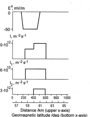
observa-Fig. 2.Latitudinal dependence of the model input parameters at the upper boundary of the region of model simulation. The meridional component of the electric fieldEx used to simulate the electron density in Fig. 1c, the flux of soft electronsI0, and the meridional component of the electric fieldExused to simulate the electron den-sity in Fig. 1d are illustrated in the top, middle, and bottom panels, respectively.
tion. However, there are still other parameters controlling the model, like the large-scale electric field, the parameters of auroral particles precipitation etc. The vertical cross sec-tion of the ionosphere shown in the top panel of Fig. 1 can be numerically reproduced by varying experimentally the un-known values of these parameters.
When selecting values of the model the following circum-stances have been taken into account. The Millstone Hill incoherent scatter radar has observed F-region ionisation de-creases in a postmeridian sector (Evans et al., 1983a,b) which are located in regions of fast ion drifts of up to 1 km/s. It is well known that such drifts are induced by electric fields of ∼50 mV/m. Therefore an efford was made to simulate the trough by defining an outer large-scale electric field which is latitudinally uniform.
Figure 1b shows a simulated electron density distribution which excludes a large- scale electric field and particle pre-cipitation. It can be seen that the observed electron density decreases smoothly from low to high latitudes, while the F2-layer peak altitude increases. Theory predicts (e.g. Ivanov-Kholodny and Nikolsky, 1969) no trough in the examined region. Further computations showed that a good agreement between the reconstructed and modelNe-values (Fig. 1c) can
be obtained by including a non-zero large-scale electric field. It was assumed that this electric field is height-independent and perpendicular to the magnetic field. Its meridional com-ponent was taken to be inhomogeneous with a maximum value 60 mV/m at the trough latitudes.
The latitudinal dependence ofExis shown in the top panel of Fig. 2. Note that Fig. 1c presents the simulated electron density distribution assuming that the zonal component of the electric fieldEyis zero.
the model trough pattern is in quite a good agreement with the observed one. However, some detailes of the compared patterns are noticeably different. In particular, the model F-layer altitudes southwards of the trough are lower than the observed heights. An attempt was made to bring the model F2-layer altitudes closer to the observed values by introduc-ing a non-zero zonal component of the electric field all over the calculated region. By settingEy = 10 mV/m, the F2-layer altitudes could then be made to come closer to the ob-served values in the southern region. At the same time, how-ever, the calculated F2-layer altitudes in the northward re-gion became higher, because the zonal field creates an up-ward plasma drift.
Fitting the experimental and model results in the poleward region of the trough was based on the results reported by Jones et al. (1997) which show that the poleward edge of the trough can be formed by soft electron precipitation. There-fore the poleward plasma distribution was simulated by in-cluding electron precipitation in the model. A better agree-ment with the observed F2-layer altitude was obtained when a zonal fieldEy= 10 mV/m was assumed together with pre-cipitation of soft electrons with an average particle energy of 0.3 keV and a flux ofI0 = 3·1013 m−2s−1 in the region poleward of the trough. The resulting model distribution of
Neis shown in Fig. 1d. The latitudinal dependence ofI0and
Ex used for simulating this distribution is presented in the second and bottom panels of Fig. 2. It can be seen that, of the three simulations, the model behaviour in Fig. 1d has the best agreement with the observations in Fig. 1a.
Since the model parameters used in Fig. 1d are consis-tent with realistic values, an attempt can be made to esti-mate the physical factors which generate the daytime plasma behaviour observed on November 17, 1995. The main fac-tor in the trough formation is a latitudinally inhomogeneous meridional component of the external electric field having enhanced values up to 60 mV/m at the trough latitudes. The inhomogeneous field is known to cause a strip of fast zonal ion drift up to 1200 m/s (Galperin et al., 1990). Calculations show that this is due to frictional plasma heating as well as due to acceleration of the reactions transforming the atomic ions O+into the molecular NO+and O+
2 which, as a result, leads to a decreased F2 layer density.
When calculating the distribution shown in Fig. 1d, two other factors have also been taken into account: the zonal component of the external electric field and the precipitation of soft electrons in the northward part of the trough. Then it was possible to make the equatorial and poleward walls of the model trough consistent with the observed ones. In particular, these factors allowed to achieve an agreement be-tween the F2 layer altitudes and the regions in the locality of the trough equatorial and poleward regions.
2.3 Trough formation during a strong evening geomagnetic activity
A severe mid-latitude geomagnetic storm occurred over the northeast of the United States and over the eastern part
of Canada during the RATE-tomographic experiment in November 1993 (Foster et al., 1994). The storm event in November 3-11, 1993 was studied by many scientists (Xin-lin et al., 1997; Bust et al., 1997). A special issue of J. Geo-phys. Res. (1998) was devoted to this event. Fortunately, a tomographic experiment was going on at that time giving F layer electron density images in the vicinity of the trough. Such a storm is almost a unique event in the evening. The receiver chain consisted of four sites located at the follow-ing latitudes: Roberval, Canada (48.42◦ N), Jay, Vermont (44.95◦N), Hanscom AFB, Massachusetts (42.45◦N), and Block Island, Rhode Island (41.17◦ N). The chain was ori-ented approximately along the meridian 288◦. The naviga-tional satellite system described in Sect. 1 was used in this experiment. The phase- difference tomography method de-scribed by Andreeva et al. (1992) was applied to calculate the ionospheric images. Fig. 3 portrays the electron density (×1012 m−3) observed at 00:41 UT on November 4, 1993 during strong geomagnetic activity (Kp = 6). Thex-axis shows the northward distance from Jay as well as the geo-magnetic latitude8.
The tomographic chain and therefore also the recon-structed image of the ionosphere shown in Fig. 3 lay ap-proximately in the geomagnetic meridian plane 20:00 MLT in the evening sector. The trough seen in the figure is not wide but it is rather deep. It is also seen that the poleward wall of the trough contains two electron density maxima sep-arated by almost 100 km in altitude and about one degree in latitude. The nothernmost tomographic site (Roberval) is located southward from the poleward edge of the trough (x = 385 km). Nevertheless, the poleward edge is well re-constructed since this region still contains rays crossing each other. Tomographic reconstructions over the northwestern USA and eastern Canada at F-region altitudes in the vicinity of the trough during the event on November 4, 1993, are also presented by Foster et al. (1994). The results reveal com-plicated inhomogeneous features of the poleward edge of the trough as seen in Fig. 3.
Tomographic observations of the F-region trough in an Scandinavian evening sector during disturbed conditions have been reported by Pryse et al. (1998). However, the poleward wall of the trough contains no peculiarities simi-lar to those in Fig. 3. It can be noted that during a strong magnetic activity withKp=6 the precipitation zone of soft electrons can move southward reaching entirely the region shown in Fig. 3 (Hardy et al., 1985).
satel-Fig. 3. Reconstructed image of the electron density (×1012m−3) observed in the vertical plane over the tomographic chain in the USA and Canada in the evening at 00:41 UT on 4 November, 1993. The inversion is made by means of the phase difference to-mographic method. The upperx-axis shows the distance on the ground (km), and the bottom axis indicates the geomagnetic lati-tude (degrees). The receiver sites from north to south are: Roberval, Canada (48.42◦N, 385 km); Jay, VT (44.95◦N, 0 km); Hanscom AFB, MA (42.45◦N,−277 km), and Block Island, RI (41.17◦N, −419 km). Only the most nothern sites are shown by open dots on the horizontal axis.
lite observations during the storm event (Foster et al., 1998). As in the previous case, the poleward wall of the trough was simulated assuming precipitating soft electrons (Jones et al., 1997).
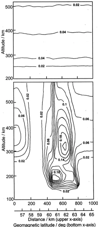
No electric field or electron precipitation was included in the first simulation. The resulting electron density is pre-sented in the top panel of Fig. 4. It is seen thatNehas no
troughs, the pattern is homogeneous with respect to latitude and varies smoothly with altitude. Next an effort was made to reproduce the observation in Fig. 3 by including an external electric field and a flux of precipitating soft electrons. These parameters have not been directly measured in the experi-ment and therefore we had freedom in their selection. The details of fitting are not described here but, in the bottom panel of Fig. 4, we only present the simulatedNedistribution
Fig. 4. Model electron density patterns (×1012 m−3) simulating the tomographic image of Fig. 3. The top panel presents the model pattern obtained without taking into account the electric field and precipitation of soft electrons. The bottom panel shows the model pattern simulated assuming an electric field with a latitudinal varia-tion and a flux of soft electron precipitavaria-tion.
Fig. 5.Latitudinal dependence of the model input parameters at the upper boundary of the region of model simulation for the pattern in the bottom panel of Fig. 4:Exis the meridional component of the electric field,I=I1+I2is the total flux of precipitating electrons, andI1andI2are the fluxes of precipitating electrons with energies of 1 keV and 0.2 keV, respectively.
observed by the satellite tomography, although some differ-ences in details can also be seen. The modelNe distribution shows a trough which is not wide but is rather deep. Two dis-tinct maxima are seen on its poleward side, which has signif-icantly higher electron density than the equatorial side. The location of the trough and the blobs of enhanced ionisation are in a good agreement with those in the observed pattern. The model simulation was calculated by assuming that the maximum value of the electric field meridional component is 50 mV/m at the trough latitudes. The fluxes of precip-itating electrons adopted wereI1 = 6·1012 m−2s−1 and
I2=3·1012m−2s−1with energies of 1 and 0.2 keV, respec-tively. Their precipitation zones were assigned to be different in width and to be shifted poleward from the zone of the max-imum electric field. The latitudinal dependence of the model parameters used in the simulation is shown in Fig. 5. Notice that the meridional component of the electric field and the fluxes and energies of the precipitating electrons are consis-tent with the experimental values described, e.g. by Hardy et al. (1985).
The simulation can be used in assessing the physical reasons for the extraordinary plasma behaviour within the trough region on November 4, 1993. The first reason is the
existence of an external poleward electric field, which varies with latitude and has enhanced values within a narrow region. Direct satellite measurements show that such an electric field often occurs during magnetic storms in the evening sector. This field can provide a fast westward subauroral ion drift (‘polarization jet’) and narrow zones of the ionisation deple-tion at the F-layer altitudes (Galperin et al., 1973; Spiro et al., 1978).
The formation of a narrow trough due to the enhanced electric field zone has been completely verified by our nu-meric calculations. Such a behaviour of the trough can be explained by the following factors. A strip of westward fast ion drift (up to 1000 m/s) initially lifted at the F-layer. The temperature within this zone is increased due to a friction of neutrals by ions, which leads to faster chemical reactions, where atomic ions O+are transformed into molecular NO+ and O+2 having a much faster dissociative recombination than the radiative recombination of O+. The increased recombi-nation finally creates a narrow trough of depleted ionization. Soft electron precipitation is the second factor which makes the poleward wall of the trough similar to the observa-tion. In particular, two enhanced density blobs with different heights and latitudes could be simulated by using precipita-tion. The proposed mechanism of trough formation can be also proved by another fact. On the night of November 3–4 the Millstone Hill incoherent scatter radar observed electron temperature enhancements higher than 4000 K at 400 km al-titude across the region of a sub-auroral ion drifts (SAID) within the trough (Foster et al., 1998). The enhanced elec-tron temperature can be caused by enhanced ion temperature induced by the frictional heating due to an increase of the electric field within the trough.
3 Interpretation of observations by means of a three-dimensional model
The two-dimensional model discussed is not a general-pur-pose tool although it has allowed us to interpret the trough formation for the cases considered. It can be used well for simulation of a trough generated due to the existence of a latitudinally inhomogeneous electric field. In paricular, the calculations by Aladjev and Mingalev (1986) show that the trough becomes deeper with increasing electric field. How-ever, sometimes our attempts to simulate the trough failed when using this model. An example of such a situation is considered later. In such cases a different, three-dimensional model was applied.
3.1 Formulation of the model
100 and 700 km measured from the ground level along the magnetic field lines for a complete day. In the model calcula-tions a field tube of plasma is traced as it moves along a con-vection trajectory through the moving neutral atmosphere. The profiles of ionospheric quantities along the geomagnetic field lines are obtained by solving the appropriate system of transport equations of the ionospheric plasma. By tracing many field tubes of plasma, it is possible to construct three-dimensional distributions of the ionospheric quantities.
The system of transport equations of ionospheric plasma in the reference frame convecting with a field tube of plasma, with itsh-axis directed upwards along the magnetic field line, can be written as follows:
∂N ∂t +
∂
∂h(N Vi)=q+qe+qp−l, (4)
miN
∂Vi
∂t +Vi ∂Vi ∂h −4 3 ∂ ∂h µ∂Vi ∂h + ∂
∂h[N k (Ti+Te)]+miNgsinI =miN
3
X
n=1 1
τin
(Un−Vi) , (5)
∂Ti ∂t = 1 M ∂ ∂h λi ∂Ti ∂h
−Vi ∂Ti
∂h + γ −1
N
∂N
∂t
+Vi∂N ∂h
Ti + 1 M
Pie+ 3
X
n=1
Pin , (6) ∂Te ∂t = 1 M ∂ ∂h λe ∂Te ∂h
−Ve ∂Te
∂h + γ −1
N
∂N
∂t
+Ve ∂N
∂h
Te+
1
M
Pei+
3
X
n=1
Pen+Q+Qe+Qp
−Lr−Lν−Le−Lf
, (7)
where N is the O+ ion number density (which is assumed to be equal to the electron density at the F-layer altitudes);
Vi is the component of the ion velocity parallel to the mag-netic field;q is the photoionisation rate;qeis the production rate due to auroral electron bombardment;qpis the
produc-tion rate due to auroral proton bombardment;l is the posi-tive ion loss rate (taking into account the chemical reactions O++O2→O+2 +O, O++N2→NO++N, O+2 +e→ O+O, and NO++e→N+O); mi is the ion mass; k is
Boltzmann constant;Ti andTeare the ion and electron
tem-peratures, respectively;gis the acceleration due to gravity;
I is the magnetic field dip angle; 1/τin is the collision
fre-quency between ion and neutral particles of typen; Un is
the field-aligned component of velocity of neutral particles of typen; M = 3/2κN,γ = 5/3; Ve is the field-aligned component of electron velocity (which is determined from
Lfare the electron cooling rates due to rotational excitation
of molecules O2and N2, due to the vibrational excitation of molecules O2and N2, due to electronic excitation of atoms O, and due to the fine structure excitation of atoms O, respec-tively.
The quantities on the right-hand sides of Eqs. (6) and (7), denoted byPab, describe the energy change rates of particles
of the type a due to elastic collisions with particles of the typeb, taking into account large differences in drift velocity. Thus these quantities contain the frictional heating caused by electric fields and thermospheric winds. In order to calcu-late the spatial distributions of various ionospheric quantities, several parameters must be given to the model, including the properties of the neutral atmosphere, the characteristics of soft electron and proton precipitation, the plasma convection pattern and so forth.
The neutral atmospheric composition, the expressions for the quantities which appear in Eqs. (4–7) as well as some of the input parameters of the model, the numerical method, the boundary conditions, as well as the other details were taken from the previous papers by Mingalev et al. (1988) and Mingaleva and Mingalev (1996).
It should be noted that this model makes it possible to obtain spatial distributions of ionospheric parameters cor-responding to stationary convection when the outer electric field has been invariable for some hours and the convection trajectories are closed as well. Therefore, this model seems to be inappropriate for simulating the trough in the our two cases, especially in the second case which is related to a storm event.
3.2 Formation of the trough during quiet evening-time con-ditions
In this section we shall consider an interpretation of the to-mographic experiment carried out in a northwest region of Russia in March-April 1990 using a chain of three receiving sites located near Verchnetulomsky (68.59◦N, 31.76◦E), not far from Murmansk, Kem in Karelia (64.95◦ N, 34.60◦E), and Moscow (55.67◦N, 37.63◦E) arranged approximately along a geomagnetic meridian (see the map e.g. in Kunitsyn et al.,1994). The chain length was 1465 km. Russian satel-lites flying from the north along the chain were used in this experiment. This selection of sites was made in order to ob-serve the trough minimum which, on the average, could be located close to Kem, the middle site of the chain, in quiet winter evenings. Electron density plots were constructed by means of the phase-difference tomography method described by Kunitsyn et al. (1994) and Foster et al. (1994).
mag-Fig. 6.Contour patterns of the electron density (×1012m−3) over the chain of receivers in Russia at 18:04 UT on 7 April 1990. The top panel shows the reconstruction obtained by means of the phase-difference tomography. The calculated pattern (bottom panel) is obtained using the three-dimensional ionospheric model. Thex -axis indicates the magnetic latitude (degrees), increasing to the left.
netic latitude, which increases to the left. At that time the tomographic cross section lay in the geomagnetic meridional plane of 20:58 MLT, i.e. in the late-evening sector. This fig-ure shows a noticeable trough having, however, a rather inter-esting poleward wall structure. Unlike the equatorial sector of the electron density distribution, which is homogeneous, the poleward region contains an isolated blob of enhanced density within the trough. Note that F region blobs have also been observed e.g. by the Chatanika incoherent-scatter radar (Rino et al., 1983). Jones et al. (1997) reported that blobs can be produced by precipitating soft electrons.
It is relevant to note that, during periods of low mag-netic activity, precipitating auroral electrons and protons can reach low geomagnetic latitudes like those of the blob in Fig. 6, however at these latitudes the particles are not intensive enough to create such a dense blob (Hardly et al., 1985, 1989). Therefore the poleward blob within the trough can-not be explained entirely by means of statistically averaged parameters of auroral fluxes. In addition, the mechanism of trough formation (the effect of the latitudinally inhomoge-neous meridional electric field of enhanced values within the trough), used for interpretation of the tomographic observa-tion performed in the USA and Canada during strong activity, cannot be applied in the latter case of low activity. Indeed, di-rect satellite measurements reveal that such a structure of the electric field is observed in the evening sector during mag-netic storms. The ionosphere was quiet on 7 April 1990, therefore the observed trough was probably formed by other mechanisms, and all our attempts at simulating the trough by means of the two-dimensional model failed. That is why the three-dimensional ionospheric model was invoked to se-lect a set of model parameters which could allow us to
re-produce the observed electron density distribution at about 21:00 MLT shown in the top panel of Fig. 6.
The basic model parameters like date, time, solar and ge-omagnetic indices were first fixed. Then we tried to fit some other characteristics which were not determined experimen-tally in order to reproduce the tomographic image. The sim-ulation is more complicated than in the previous two cases. This is because several quantities (electric field, precipitation zones of the particles and their energetic values, neutral wind velocity etc.) need to be defined in three dimensions. The three-dimensional model takes into accout the plasma con-vection, and therefore results in one place depend on input parameters defined elsewhere. Again we neglect the detailed description of the calculations and only investigate the simu-lation results shown in the bottom panel of Fig. 6, which is the best fit to the observed pattern in the top panel. In gen-eral, the model pattern contains the basic spatial features of the observed complicated trough, although the patterns dif-fer in some details. The location of the simulated trough and the Ne values on both its sides are consistent with the
ex-perimental electron density values. The model pattern also shows a blob of enhanced density which is, however, located at higher altitudes than in the tomographic plot.
The most complicated task in modelling was reproducing the required trough width and its location. The main model input parameter affecting the trough width and its location turned out to be the spatial distribution of the electric field. TheNedistribution shown in the bottom panel of Fig. 6 has been obtained by defining an external electric field consist-ing of a combination of two empirical models: (1) the con-vection field at polar latitudes was defined by the model of B described by Heppner (1977); (2) the field at subauroral and middle latitudes was calculated by means of the model developed by Richmond (1976) and Richmond et al. (1980). Figure 7 presents plasma convection trajectories based on this field definition. The appropriate 3-D distribution of the
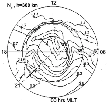
Nevalues at the levelh=300 km is illustrated in Fig. 8. The
physi-Fig. 7.Plasma convection trajectories derived from the combination of patternB of the empirical convection model at polar latitudes by Heppner (1977) and the empirical model of ionospheric electric fields at middle latitudes by Richmond (1976) and Richmond et al. (1980). The trajectories are depicted in the fixed Sun-Earth refer-ence frame. Values of the magnetic local time (MLT) and magnetic colatitude are indicated on the plot. The arrows indicate the direc-tion of the convecdirec-tion flow.
cal reasons which create the plasma distribution in the trough region, in particular the trough location and its width within the evening sector on 7 April 1990, can be deduced from our analysis. The results are in agreement with the stagnation mechanism of the trough as proposed earlier by Spiro et al. (1978) and Collis and Haggstrom (1988).
The results presented in the bottom panel of Fig. 6 and in Fig. 8 were obtained with the following input parameters. The shape of the precipitation zone as well as the particle en-ergies were taken from the statistical models by Hardy et al. (1985, 1989). The horizontal component of the neutral wind was consistent with the neutral wind measurements by Meri-wether et al. (1973) at 300 km altitude. It should be noted that the irregularity located on the trough poleside wall of the calculatedNepattern (bottom panel of Fig. 6) was created by defining an irregularity at these latitudes within the distribu-tion of the neutral wind meridional component. Therefore, these two model parameters (auroral particles precipitation and the neutral wind) have provided the model electron den-sity values consistent with the experimentalNe values and
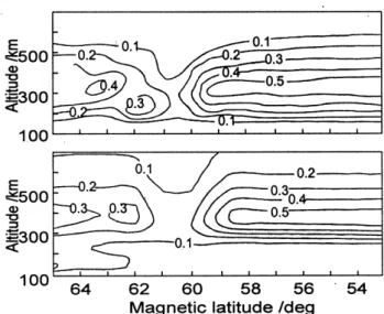
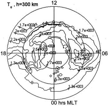
the appropriate irregularity to arise on the trough poleward wall. In addition to the electron density, the 3-D mathemati-cal model also gives other parameters, in particular the elec-tron and ion temperatures. The temperatures at 300 km al-titude corresponding to the electron density image of Fig. 8 are shown in Figs. 9 and 10. The patterns presented in Figs. 8–10 reproduce large-scale irregularities similar to other
ob-Fig. 8. Simulated distribution of the electron concentration (×1012m−3) ath=300 km. The projection of the vertical plane shown in Fig. 6 at MLT = 21:00 is presented by the bold line.
servations at high latitudes. The pattern of Fig. 8 clearly re-veals a ’tongue’ of enhanced electron density extending from dayside to nightside over the polar cap. The trough is seen on the nightside. A trough is also noticeable on the dayside, but there it is located much closer to the pole. The distribu-tion ofTi (Fig. 9) shows a feature which is often observed
experimentally. A spot of enhancedTi values, or a hot spot
ofTi, occurs at 15◦–30◦colatitudes of the morning sector.
This spot is known to be created by frictional heating due to enhanced values of the convectional electric field. The calculatedTe distribution (Fig. 10) is also quite distinctive
due to the hot spots in the morning and at night. The origin of these spots has been considered in detail by Mingaleva and Mingalev (1998).
In conclusion, the chosen model parameters give the main features of the observed two-dimensional electron density images observed on 7 April 1990 (the top panel of Fig. 6). The simulated pattern contains the basic large-scale irregu-lar structures which are in agreement with the experimental data. Hence the proposed interpretation of the tomographic images from 7 April 1990 seems to be valid.
4 Conclusion
Fig. 9.Simulated pattern of the ion temperature (in K) ath=300 km.
in 1993, a campaign in Scandinavia in 1995, and a tomo-graphic experiment in Russia in 1990. The images of elec-tron density presented display some interesting features of the F-region trough. Model calculations of an event observed during low daytime geomagnetic activity on 17 November 1995 have been performed. The tomographic image shows a well-formed trough occurring in the subauroral F-region. The simulation shows that such a pattern can be caused by the following factors: (1) meridional component of the ex-ternal electric field which has a latitudinal variation with a peak value up to 60 mV/m at trough latitudes; (2) constant zonal component of the external electric field with a value 10 mV/m; and (3) precipitation of soft electrons at the pole-ward boundary of the trough with an average particle energy of 0.3 keV.
Another tomographic measurement made on 4 Novem-ber 1993 during strong geomagnetic activity in the evening displays a complicated image of the subauroral ionosphere, which contains a narrow deep trough and two blobs of en-hanced density at its northern edge. This behaviour can be caused by an external electric field with a meridional com-ponent up to 50 mV/m within a narrow strip in the trough re-gion, as well as by precipitating soft electrons which have av-erage energies of 1 and 0.2 keV and fluxes of 6·1012m−2s−1 and 3·1012m−2s−1. The two precipitation zones are located polewards of the trough and they have different extents.
The three-dimensional ionospheric model has been ap-plied to simulate a tomographic image on 7 April 1990. This observation displays a clear trough during quiet evening con-ditions. A model simulation of this event shows that the ob-served electron density structure can be formed by the fol-lowing mechanism. Due to the electric field in a narrow transition zone of the convection pattern, the convection field
Fig. 10.Simulated distribution of the electron temperature (in K) at
h=300 km.
does not predominate over the corotation field and the plasma convection trajectories make reversal points in this region. The electric field is weak in the vicinity of the reversal points and therefore the plasma stays there for a long time. Thus the number of charged particles in the unilluminated night-side ionosphere can be essentially reduced even by the slow F-region recombination. In this manner a trough can be cre-ated within the late evening and pre-midnight sector.
The simulations shown make it possible to evaluate the physical reasons for the observed structures of the iono-spheric electron density. Generally speaking, the observa-tions do not allow unique conclusions regarding the physi-cal reasons to be made, and therefore our discussion should be considered only as a single possible explanation. Nev-ertheless, our model predictions are not unusual since simi-lar ideas on the physical and chemical ionospheric processes have been presented before. In the simulations, a large num-ber of other combinations of model parameters has been tried which could not reproduce experimental results. Hence, the problems presented seem only to have these noncontradic-tory model solutions although further studies on a routine basis are needed to test the model predictions.
Acknowledgement. The authors are grateful to Y. A. Melnichenko, S. M. Chernyakov, M. Lehtinen, T. Nygr´en, J. Pirttil¨a, T. Ulich and E. Saviaro for assistance in making the measurements in Russia and Scandinavia; to V. E. Kunitsyn, E. S. Andreeva, and M. Markkanen for their help in data processing. We are also grateful to J. C. Foster in arranging the RATE-93 tomographic measurement in the USA and Canada.
polar-cap regions during magnetospheric substorms, Geomagn. Aeron., 29, 38–44, 1989 (in Russian).
Andreeva, E. S., Kunitsyn, V. E., and Tereshchenko, E. D., Phase-difference radio tomography of the ionosphere, Ann. Geophysi-cae, 10, 849–855, 1992.
Austen, J. R., Franke, S. J., Liu, C. H., and Yeh, K. C., Applica-tion of computerized tomography techniques to ionospheric re-search, in Radio beacon contribution to the study of ionisation and dynamics of the ionosphere and corrections to geodesy, Ed. A. Tauriainen, University of Oulu, Finland, Part 1, 25–35, 1986. Austen, J. R., Franke, S. J., and Liu, C. H., Ionospheric imaging using computerized tomography, Radio Sci., 23, 299–307, 1988. Bust, G. S., Gaussiran II, T. L., and Coco, D. S., Ionospheric ob-servations of the November 1993 storm, J. Geophys. Res., 102, 14293–14304, 1997.
Collis, P. N. and Haggstrom, I., Plasma convection and auroral precipitation processes associaated with the main ionospheric trough at high latitudes, J. Atmos. Terr. Phys., 50, 389–404, 1988.
Evans, J. V., Holt, J. M., Oliver, W. L., and Wand, R. H., The fossil theory of nighttime high latitude F-region troughs, J. Geophys. Res., 88, 7769–7782, 1983a.
Evans, J. V., Holt, J. M., and Wand, R. H., On the formation of daytime troughs in the F-region at high latitudes, Geophys. Res. Lett., 10, 405–410, 1983b.
Foster, J. C., Buonsanto, M. J., Holt, J. M., Klobuchar, J. A., Fougere, P., Pakula, W., Raymund, T. D., Kunitsyn, V. E., Andreeva, E. S., Tereshchenko, E. D., and Khudukon, B. Z., Russian-American tomography experiment, J. Imag. Syst. Tech-nol., 5, 148–159, 1994.
Foster, J. C., Cummer, S., and Inan, U. S., Midlatitude particle and electric field effects at the onset of the November 1993 geomag-netic storm, J. Geophys. Res., 103, 26359–26366, 1998. Galperin, Y. I., Ponomarev, V. N., and Zosimova, A. G., Direct
measurements of the ion drift velocity during a magnetic storm, Kosm. Issled., 11, 273–296, 1973 (in Russian).
Galperin, Y. I., Sivtseva, L. D., Philippov, V. M., and Khalipov, V. L., The subauroral upper ionosphere, Nauka, Siberian Depart-ment, Novosibirsk, 1990 (in Russian).
Hardy, D. A., Gussenhoven, M. S., and Holeman, E., A statisti-cal model of auroral electron precipitation, J. Geophys. Res., 90, 4229–4248, 1985.
Hardy, D. A., Gussenhoven, M. S., and Brautigam, D., A statistical model of auroral ion precipitation, J. Geophys. Res., 94, 370– 392, 1989.
Heppner, J. P., Empirical models of high-latitude electric fields, J. Geophys. Res., 82, 1115–1125, 1977.
Ivanov-Kholodny, G. S., and Nikolsky, G. M., The sun and iono-sphere, Nauka, Moscow, 1969 (in Russian).
Jones, D. G., Walker, I. K., and Kersley, L., Structure of the pole-ward wall of the trough and the inclination of the geomagnetic field above the EISCAT radar, Ann. Geophysicae, 15, 740–746, 1997.
J. Geophys. Res., 103, A11, 1998.
Kunitsyn, V. E., Tereshchenko, E. D., Andreeva, E. S., Galinov, A. V., Melnitchenko, Y. A., Stepanov, V. A., Philimonov, M. A.,
lite radiotomography, J. Imag. Syst. Technol., 5, 112–127, 1994. Kunitsyn, V. E., Tereshchenko, E. D., Andreeva, E. S., Khudukon, B. Z., and Melnichenko, Y. A., Radiotomographic investigations of ionospheric structures at auroral and middle latitudes, Ann. Geophysicae, 13, 1242–1253, 1995.
Markkanen, M., Lehtinen, M., Nygren, T., Partilla, J., Henelius, P., Vilenius, E., Tereshchenko, E. D., and Khudukon, B. Z., Bayesian approach to satellite radio tomography with applica-tions in the Scandinavian sector, Ann. Geophysicae, 13, 1277– 1287, 1995.
Meriwether, J. M., Heppner, J. P., Stolaric, J. D., and Wescott, E. M., Neutral winds above 200 km at high latitudes, J. Geophys. Res., 78, 6643–6661, 1973.
Mingalev, V. S. and Aladjev, G. A., The dependence of ionospheric ionization density on neutral atmosphere density, in Radiowaves propagation in disturbed ionosphere, Eds. N. A. Gorokhov, A. K. Dudakov, N. V. Kalitenkov, and B. V. Tkachenko, Kola Branch of the USSR Academy of Sciences, Apatity, 103–113, 1983 (in Russian).
Mingalev, V. S., Krivilev, V. N., Yevlashina, M. L., and Mingaleva, G. I., Numerical modeling of the high-latitude F-layer anomalies, PAGEOPH, 127, 323–334, 1988.
Mingaleva, G. I. and Mingalev, V. S., The formation of electron tem-perature hot spots in the main ionospheric trough by the internal processes, Ann. Geophysicae, 14, 816–825, 1996.
Mingaleva, G. I. and Mingalev, V. S., Three-dimensional mathemat-ical model of the polar and subauroral ionosphere, in Modelling of the upper polar atmosphere processes, Eds. V. E. Ivanov, Ya. A. Sakharov, and N. V. Golubtsova, PGI, Murmansk, 251–265, 1998 (in Russian).
Moffett, R. J., and Quegan, S., The mid-latitude trough in the elec-tron concentration of the ionospheric F-layer: a review of obser-vations and modelling, J. Atmos. Terr. Phys., 45, 315–343, 1983. Pryse, S. E., Kersley, L., Williams, M. J., and Walker, I. K., The spatial structure of the dayside ionospheric trough, Ann. Geo-physicae, 16, 1169–1179, 1998.
Raymond, T. D., Austen, J. R., Franke, S. J., Liu, C. H., Klobuchar, J. A., and Stalker, J., Application of computerized tomography to the investigation of ionospheric structures, Radio Sci., 25, 771– 789, 1990.
Richmond, A. D., Electric field in the ionosphere and plasmasphere on quiet days, J. Geophys. Res., 81, 1447–1450, 1976.
Richmond, A. D., Blanc, M., Emery, B. A., Wand, R. H., Fejer, B. G., Woodman, R. F., Ganguly, S., Amayenc, P., Behnke, R. A., Calderon, C., and Evans, J. V., An empirical model of quiet-day ionospheric electric fields at middle and low latitudes, J. Geo-phys. Res., 85, 4658–4664, 1980.
Rino, C. L., Livingston, R. C., Tsunoda, R. T., Robinson, R. M., Vickrey, J. F., Senior, C., Cousins, M. D., and Owen, J., Recent studies of the structure and morphology of auroral zone F region irregularities, Radio Sci., 18, 1167–1180, 1983.
Rodger A. S., Moffett, R. J., and Quegan, S., The role of ion drift in the formation of ionisation troughs in the mid-and high-latitude ionosphere – a review, J. Atmos. Terr. Phys, 54, 1–30, 1992. Spiro, R. W., Heelis, R. A., and Hanson, W. B., Ion convection and
Geophys. Res., 83, 4255–4263, 1978.
Xinlin Li, Baker, D. N., Temerin, M., Cayton, T. E., Reeves, E. G. D., Christensen, R. A., Blake, J. B., Looper, M. D.,