Artigo
*e-mail: [email protected]
PREDICTING THE BOILING POINT OF PCDD/Fs BY THE QSPR METHOD BASED ON THE MOLECULAR DISTANCE-EDGE VECTOR INDEX
Long Jiaoa,*, Xiaofei Wanga, Shan Binga, Zhiwei Xueb and Hua Lic
aCollege of Chemistry and Chemical Engineering, Xi’an Shiyou University, Xi’an 710065, China bNo.203 Research lnstitute of Nuclear industry, Xianyang, 712000, China
cCollege of Chemistry and Materials Science, Northwest University, Xi’an 710069, China
Recebido em 17/10/2014; aceito em 17/12/2014; publicado na web em 05/03/2015
The quantitative structure property relationship (QSPR) for the boiling point (Tb) of polychlorinated dibenzo-p-dioxins and polychlorinated dibenzofurans (PCDD/Fs) was investigated. The molecular distance-edge vector (MDEV) index was used as the structural descriptor. The quantitative relationship between the MDEV index and Tb was modeled by using multivariate linear regression (MLR) and artificial neural network (ANN), respectively. Leave-one-out cross validation and external validation were carried out to assess the prediction performance of the models developed. For the MLR method, the prediction root mean square relative error (RMSRE) of leave-one-out cross validation and external validation was 1.77 and 1.23, respectively. For the ANN method, the prediction RMSRE of leave-one-out cross validation and external validation was 1.65 and 1.16, respectively. A quantitative relationship between the MDEV index and Tb of PCDD/Fs was demonstrated. Both MLR and ANN are practicable for modeling this relationship. The MLR model and ANN model developed can be used to predict the Tb of PCDD/Fs. Thus, the Tb of each PCDD/F was predicted by the developed models.
Keywords: QSPR; molecular distance-edge vector index; PCDD/Fs; boiling point.
INTRODUCTION
Polychlorinated dibenzo-p-dioxins and polychlorinated diben-zofurans (PCDD/Fs) are two series of persistent organic pollutants which have been detected in almost all compartments of the global ecosystem. These chemicals have gained much attention due to their toxicity, environmental persistence, tendency to accumulate through the food chain, and the risk to human health. PCDD/Fs are not produced intentionally and do not serve any useful purpose. They are formed as byproducts of many industrial and combustion processes. PCDD/Fs are semi-volatile compounds. After released into the atmosphere, they are likely to transfer to other environmental compartments such as soil, water, sediments and their resident biota where they can last for years before degradation.1-5
The boiling point (Tb) is an important property for studying the
volatility of PCDD/Fs, which is correlated with the fate, transport, and transformation of PCDD/Fs in the environment. Boiling point is also a significant factor in determining physico-chemical proper-ties of PCDD/Fs, such as vapor pressure, octanol/water partitioning coefficient and aqueous solubility.6-9 A quantitative study on the T
b
is necessary to understand the environmental behavior of PCDD/Fs. Experimentally determining the Tb of PCDD/Fs is still a hard work
because of the complexity of analytical methods, high cost of experi-ments and lack of the standards.7 In addition, the measurement of
boiling point of PCDD/Fs is hazardous due to the high vapor pressures involved.6 Up to now, the T
b has not been experimentally determined
for each PCDD/F congener.
Quantitative structure property relationship (QSPR) method is safe, fast, convenient and cost-effective for predicting the property of compounds. Therefore, it is worthwhile to develop an accurate and easy-to-use QSPR model for predicting the Tb of PCDD/Fs.
Topological index is a kind of structural descriptor which is often used in QSPR researches. It can efficiently describe the structure of
a molecule without detailed molecular orbital calculations. It is use-ful because, despite its mathematical simplicity, topological index is able to differentiate molecules with different structures.10,11 The
aim of this work is developing the QSPR model for the Tb of PCDD/
Fs based on the topological index. Molecular distance-edge vector (MDEV) index12-17 was used as the structural descriptor of PCDD/
Fs. Multivariate linear regression (MLR) and linear artificial neural network (L-ANN) were employed to model the quantitative relation-ship between the Tb and MDEV index of PCDD/Fs.
EXPERIMENTAL
Data set
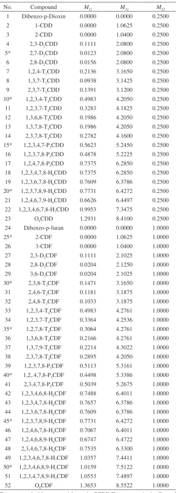
The MDEV index was calculated according to the approach pre-sented in the followed section. The MDEV index of the 52 PCDD/ Fs, of which the Tb value is known, is listed in Table 1. The observed
Tb value of these PCDD/Fs was taken from the references 7,18 and
listed in Table 2.
Root mean square relative error (RMSRE) was used to indicate the prediction performance of the developed models. The RMSRE is defined as Equation 1:
2 ( )REi RMSRE
n
=
∑
,
b,pred b,obsb,obs
100%
i
T T
RE T
−
= × (1)
where REi is the relative error of the ith sample; n is the number of samples; Tb,pred and Tb,obs is the predicted Tb and observed Tb
respectively.
MDEV index
is considered as a point and each chemical bond is considered as an edge. The relative electronegative of each chlorine atom and benzene ring is defined as 1. Correspondingly, the MDEV index is defined as Equation 2:
2 1
kl
j i≥ ik jl, M
d
=
∑
(k, l =1,2 and l ≥ k) (2)In Equation 2, k or l is the type of atoms (k =1 or l =1 denotes the chlorine atom, and k =2 or l =2 denotes the benzene ring); Items i and j are the coding number of a chlorine atom or a benzene ring. Additionally, i and j belong to the kth and lth type respectively. The dik,jl represents the nearest relative distance between the ith and jth atom. For example, di1,j1 indicates the shortest relative distance
be-tween the ith and jth chlorine atom. The relative distance between the two adjacent non-hydrogen atoms is defined as d = 1. According to Equation 2, there are three elements, M11, M12 and M22, in the MDEV
index for a PCDD/F molecule. For instance, the MDEV index of 2, 3, 7-CDD should be calculated as follows:
1391 . 0 8 1 9 1 3
1 2 2 2
11 =
+ + = M 12 . 3 5 1 1 1 5 1 1 1 5 1 1
1 2 2 2 2 2 2
12 =
+ + + + + = M 25 . 0 2 1 2 22 =
=
M (3)
The MDEV index of 2, 4, 6-CDF should be calculated as following: 1181 . 0 6 1 6 1 4
1 2 2 2
11 =
+ + = M 1875 . 3 4 1 1 1 4 1 1 1 4 1 1
1 2 2 2 2 2 2
12 =
+ + + + + = M 1 1 1 2 22 =
=
M (4)
Artificial neural network
ANN14-17,19-29 is a multivariate calibration approach capable of
modeling various complex functions. Its basic processing unit is the neuron (node). An ANN comprises a number of neurons organized in different layers. Linear artificial neural network,25-29 is a kind of
neural network having no hidden layers, but an output layer with fully linear neurons (that is, linear neurons with linear activation function). It is the simplest ANN and is usually used to develop linear model. It is often used as a good benchmark against which to compare the prediction performance of other methods. Although a number of multivariable calibration problems cannot be solved or solved well by L-ANN, many others can. It is common to find that a problem which was perceived to be difficult and non-linear can actually be solved satisfactorily by using L-ANN.
In L-ANN, the neurons between the input and output layers fully connected, while the neurons in the same layer do not. Figure 1 shows the basic architecture of the L-ANN.
In Figure 1, xi( i =1, 2, …, n), yj ( j =1, 2,… , m) and wij is the input variables, output variables and the element of connection weight matrix W respectively. And bj is the bias vector, which corresponds to the thresholds. The symbol fact( ) means the activation function.
Table 1. MDEV index of the investigated PCDD/Fs
No. Compound M11 M12 M22
1 Dibenzo-p-Dioxin 0.0000 0.0000 0.2500
2 1-CDD 0.0000 1.0625 0.2500
3 2-CDD 0.0000 1.0400 0.2500
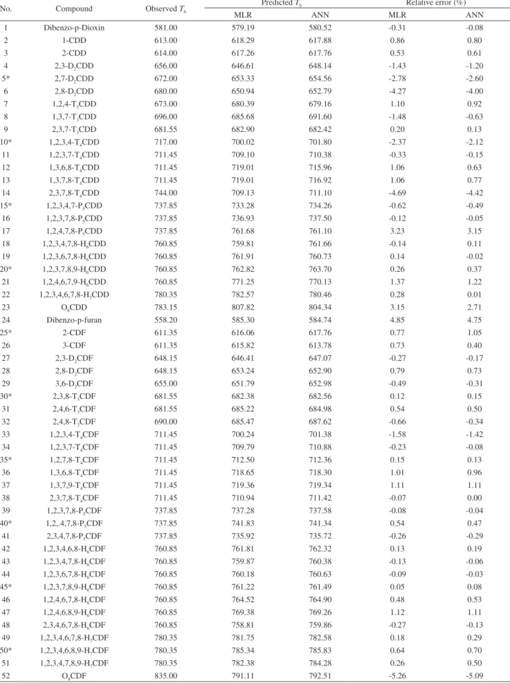
Table 2. Result of leave-one-out cross-validation and external validation
No. Compound Observed Tb Predicted Tb Relative error (%)
MLR ANN MLR ANN
1 Dibenzo-p-Dioxin 581.00 579.19 580.52 -0.31 -0.08
2 1-CDD 613.00 618.29 617.88 0.86 0.80
3 2-CDD 614.00 617.26 617.76 0.53 0.61
4 2,3-D2CDD 656.00 646.61 648.14 -1.43 -1.20
5* 2,7-D2CDD 672.00 653.33 654.56 -2.78 -2.60
6 2,8-D2CDD 680.00 650.94 652.79 -4.27 -4.00
7 1,2,4-T3CDD 673.00 680.39 679.16 1.10 0.92
8 1,3,7-T3CDD 696.00 685.68 691.60 -1.48 -0.63
9 2,3,7-T3CDD 681.55 682.90 682.42 0.20 0.13
10* 1,2,3,4-T4CDD 717.00 700.02 701.80 -2.37 -2.12
11 1,2,3,7-T4CDD 711.45 709.10 710.38 -0.33 -0.15
12 1,3,6,8-T4CDD 711.45 719.01 715.96 1.06 0.63
13 1,3,7,8-T4CDD 711.45 719.01 716.92 1.06 0.77
14 2,3,7,8-T4CDD 744.00 709.13 711.10 -4.69 -4.42
15* 1,2,3,4,7-P5CDD 737.85 733.28 734.26 -0.62 -0.49
16 1,2,3,7,8-P5CDD 737.85 736.93 737.50 -0.12 -0.05
17 1,2,4,7,8-P5CDD 737.85 761.68 761.10 3.23 3.15
18 1,2,3,4,7,8-H6CDD 760.85 759.81 761.66 -0.14 0.11
19 1,2,3,6,7,8-H6CDD 760.85 761.91 760.73 0.14 -0.02
20* 1,2,3,7,8,9-H6CDD 760.85 762.82 763.70 0.26 0.37
21 1,2,4,6,7,9-H6CDD 760.85 771.25 770.13 1.37 1.22
22 1,2,3,4,6,7,8-H7CDD 780.35 782.57 780.46 0.28 0.01
23 O8CDD 783.15 807.82 804.34 3.15 2.71
24 Dibenzo-p-furan 558.20 585.30 584.74 4.85 4.75
25* 2-CDF 611.35 616.06 617.76 0.77 1.05
26 3-CDF 611.35 615.82 613.78 0.73 0.40
27 2,3-D2CDF 648.15 646.41 647.07 -0.27 -0.17
28 2,8-D2CDF 648.15 653.24 652.90 0.79 0.73
29 3,6-D2CDF 655.00 651.79 652.98 -0.49 -0.31
30* 2,3,8-T3CDF 681.55 682.38 682.56 0.12 0.15
31 2,4,6-T3CDF 681.55 685.22 684.98 0.54 0.50
32 2,4,8-T3CDF 690.00 685.47 687.62 -0.66 -0.34
33 1,2,3,4-T4CDF 711.45 700.24 701.38 -1.58 -1.42
34 1,2,3,7-T4CDF 711.45 709.79 710.88 -0.23 -0.08
35* 1,2,7,8-T4CDF 711.45 712.50 712.36 0.15 0.13
36 1,3,6,8-T4CDF 711.45 718.65 718.30 1.01 0.96
37 1,3,7,9-T4CDF 711.45 719.36 719.34 1.11 1.11
38 2,3,7,8-T4CDF 711.45 710.94 711.42 -0.07 0.00
39 1,2,3,7,8-P5CDF 737.85 737.28 737.58 -0.08 -0.04
40* 1,2,.4,7,8-P5CDF 737.85 741.83 741.34 0.54 0.47
41 2,3,4,7,8-P5CDF 737.85 735.92 735.72 -0.26 -0.29
42 1,2,3,4,6,8-H6CDF 760.85 761.81 762.32 0.13 0.19
43 1,2,3,4,7,8-H6CDF 760.85 759.87 760.38 -0.13 -0.06
44 1,2,3,6,7,8-H6CDF 760.85 760.18 760.63 -0.09 -0.03
45* 1,2,3,7,8,9-H6CDF 760.85 761.22 761.49 0.05 0.08
46 1,2,4,6,7,8-H6CDF 760.85 764.52 764.90 0.48 0.53
47 1,2,4,6,8,9-H6CDF 760.85 769.38 769.26 1.12 1.11
48 2,3,4,6,7,8-H6CDF 760.85 758.81 759.86 -0.27 -0.13
49 1,2,3,4,6,7,8-H7CDF 780.35 781.75 782.58 0.18 0.29
50* 1,2,3,4,6,8,9-H7CDF 780.35 785.34 785.83 0.64 0.70
51 1,2,3,4,7,8,9-H7CDF 780.35 782.38 784.28 0.26 0.50
52 O8CDF 835.00 791.11 792.51 -5.26 -5.09
Before the training procedure, input and output variables are nor-malized. When the network is executed, it effectively multiplies the input variables by the weight matrix W, and then adds the bias vector bj. Hence, the post synaptic potential (PSP) function of the neuron should be described as Equation 5:
j i ij j
1 n
i
v x w b
=
=
∑
+ . (5)Generally, the activation function used in L-ANN is a linear function:
yj=vj (6)
Because there are no non-linear functions and hidden neurons in the network, L-ANN is good at solving linear problems. Actually, training a linear network means finding the optimal value of the weight matrix W to minimize the root mean squared error of the calibration set. In order to reach this goal, the known samples are always divided into two subsets: a training set and a verification set. The network is trained by using the training set, and is tested after each epoch by using the verification set. The training is terminated once deterioration in the root mean squared error of verification set is occurred. The over-fitting and over-learning are avoided in this way. Although the verification set is used to find the best network setting, actually, training algorithms do not use the verification set to adjust network weights. Standard pseudo-inverse linear optimi-zation algorithm26 is usually used to train the network. This
algo-rithm uses the singular value decomposition technique to calculate the pseudo-inverse of the matrix needed to set the weights in the linear output layer, so as to find the least mean squared solution. Essentially, it guarantees to find the optimal setting for the weight matrix in a linear layer.
The main difference between MLR and L-ANN is the optimi-zation algorithm. In MLR, the goal of least square algorithm is to find the minimal sum of squared residuals of the training set. As for L-ANN, the goal of training algorithm is to minimize the root mean squared error of verification set.26 Thus, the prediction ability of
L-ANN is usually better than that of MLR.
Leave-one-out cross-validation
Leave-one-out cross-validation15-17,30 is a commonly used
al-gorithm for estimating the predictive performance and robustness of a multivariable calibration model. Usually, practical calibration experiments have to be based on a limited set of available samples.
The idea behind the leave-one-out cross validation algorithm is to predict the property value of each sample in turn with the calibration model which is developed from the other samples. When applying the algorithm to a dataset including n samples, the calibration modeling is performed n times, each time using (n-1) samples for modeling and one sample for testing. Hence, the procedure of leave-one-out cross validation can be divided into n segments. In each segment i (i = 1, … , n), there are three steps: (1) taking sample i out as tempo-rary ‘test set’, which is not used to establish the calibration model, (2) developing a calibration model with the rest (n-1) samples, (3) testing the established model with sample i, computing and storing the prediction error of the sample. The advantage of leave-one-out cross validation over random sub-sampling is that each sample is used for validation exactly once. Although leave-one-out cross-validation is an effective and commonly used method, there is still the risk of overestimating the predictive performance and robustness of a model when using this method. It is common to use two or more validation methods for estimating a calibration model. The risk of overestimation can be effectively lessened in this way.
External validation
External validation17,25,30 is an algorithm which has been often
used to assess the predictive ability of a calibration model. When using this algorithm, working dataset is split into two subsets: a calibration set, which is used to develop the calibration model, and a test set, which is used to assess the predictive ability of the devel-oped model. Obviously, test set is designed to give an independent assessment of the predictive performance of the developed model. It is not used in developing the model at all, and hence is independent of the calibration set. Generally, the calibration set and test set are randomly selected from the working dataset.
Software
All the calculation was done by using subroutines developed in MATLAB (Ver.7.0). The computation was performed on a personal computer equipped with an i5-2450M processor.
RESULTS AND DISCUSSION
The MDEV index of PCDD/Fs was calculated. The result is listed in Table 1 and Table 3. Clearly, the MDEV index of different PCDD/F molecules is quite different. It is demonstrated that MDEV index can describe the structural differences among these compounds. It is reasonable to use the MDEV index as the structural descriptor to develop the QSPR model of PCDD/Fs.
MLR model
Generally, a simple model should always be chosen in preference to a complex model, if the latter does not fit the data better. Thus, we firstly investigated whether MLR is feasible to model the quan-titative relationship between the MDEV index and Tb of PCDD/Fs.
The MDEV index was used as the independent variable and the Tb
was used as the dependent variable to develop the regression model. In order to assess the predictive ability of the developed model, two validation methods, leave-one-out cross validation and external validation, were conducted. The 52 samples shown in Table 1 were randomly split into two groups: Group I, which comprises 42 samples, and Group II, which comprises 10 samples.
Leave-one-out cross validation was applied to Group I. The result is presented in Table 2. As shown in Table 2, the predicted
Tb is in consistent with the observed Tb. For the 42 compounds,
the RMSRE of prediction is 1.77. Moreover, the predicted Tb were
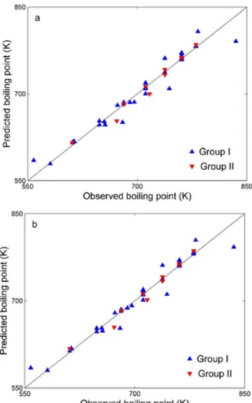
plotted versus the observed Tb (as shown in Figure 2a) and the plot
shows a linear relationship (y = 0.9904 x + 7.9881 with R= 0.9819) between the predicted and observed Tb. Subsequently, external
validation was carried out to further assess the predictive ability of the MLR model. In this procedure, the model was established by using all the 42 compounds in Group I as the calibration set. The obtained regression equation is: Tb = -60.50 M11 + 35.78 M12 – 2.14
M22 + 580.20. The R
2, Standard error of the estimate (S.E.) and F
value of the regression model is 0.9672, 10.426 and 368.8 respec-tively. The value of F [F < F0.01 (N, N-3)] indicates that MDEV
index is significant to Tb. It is reasonable to develop a regression
model between the MDEV index and Tb. The S.E. is significantly
smaller than the sample mean of Tb. It is shown that the obtained
regression equation fits the data well. Then, the Tb of the samples in
Group II was predicted by using the obtained regression equation. The prediction result is shown in Table2. As shown in the table, the predicted Tb is in good accordance with the observed Tb. For the 10
compounds, the prediction RMSRE is 1.23. The plot of predicted Tb versus observed Tb is shown in Figure 2a, which shows a linear
relationship (y = 0.9957 x + 0.9347 with R= 0.9864) between the predicted and observed Tb.
The result of the leave-one-out cross validation and external validation demonstrates that the MDEV index of the investigated
PCDD/Fs is quantitatively related to their Tb. In previous researches,
MDEV index has been just used as the structural descriptor to de-velop the QSPR model of the compounds which include the same basic structure, such as the boiling points model of alcohols,13 the
gas/particle partition coefficient model of PCBs,17 etc.14-16 The basic
structure of polychlorinated dibenzo-p-dioxins is different from the basic structure of polychlorinated dibenzofurans. Thus, it is shown that MDEV index can be used as the structural descriptor to establish the QSPR model for the compounds with different basic structures. In addition, the validation result demonstrates that MLR is practicable for modeling the quantitative relationship between the MDEV index and Tb of PCDD/Fs. Obviously, a linear QSPR model based on MDEV
index is able to predict the Tb of PCDD/Fs. Thus, an MLR model was
developed by using all the 52 PCDD/Fs listed in Table 1. The obtai-ned regression equation is: Tb = –59.68 M11 + 35.49 M12 – 4.99 M22
+ 583.46 The R2, S.E. and F value of the regression model is 0.9679,
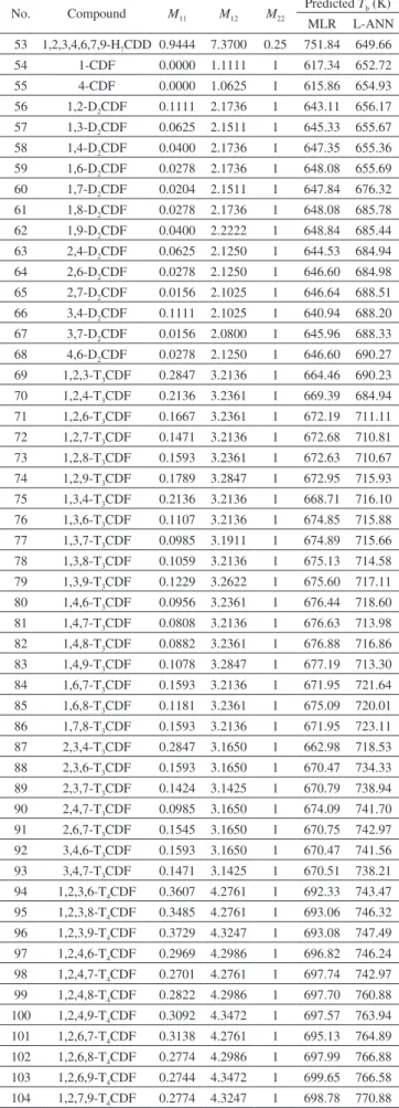
10.81 and 477.1 respectively. The Tb of the other 53 PCDDs and 107
PCDFs was then predicted by using this regression equation. The result is shown in Table 3. The Tb value of these PCDD/Fs has not
been experimentally determined as yet. Thus, our prediction result can be used as an estimation Tb of these compounds.
L-ANN model
L-ANN is another commonly used linear calibration method in QSPR studies. Thus, we investigated whether a better model can be established by using L-ANN. A 3-1 L-ANN (i.e. 3 input varia-bles and 1 output variable in the network) was used to develop the calibration model. The MDEV index and Tb was used as input and
output variables respectively. In each run of ANN, ten samples were randomly selected and used as the verification set. Leave-one-out cross validation and external validation were carried out to assess the prediction performance of the developed model. Group I was still used to complete the leave-one-out cross validation. The result of leave-one-out cross validation is listed in Table 2. As shown in the table, the predicted Tb is in good agreement with the observed
Tb. For the 42 compounds, the RMSRE of prediction is 1.65. The
predicted Tb were plotted versus the observed Tb (shown in Figure
2b) and the plot shows a linear relationship (y = 0.9893 x + 9.0119 with R= 0.9847) between the predicted and observed Tb. Then, all
the 52 samples were used to complete the external validation. An L-ANN model was developed by using the 42 samples of Group I as the calibration set. In the training procedure, verification set comprises ten randomly selected samples. The Tb of the samples in
Group II was predicted by using the obtained network. The result of external validation is also shown in Table 2. Obviously, the pre-dicted Tb is also in good agreement with the observed Tb. For the
ten samples, the prediction RMSRE is 1.16. The plot of predicted Tb versus observed Tb (shown in Figure 2b) shows that there is a
linear relationship (y = 0.9966x + 0.9747 with R=0.9875) between the predicted and observed Tb. Obviously, the prediction accuracy
of the L-ANN model is slightly higher than that of the MLR model. Using L-ANN is slightly better than MLR in modeling the quan-titative relationship between the MDEV index and Tb of PCDD/
Fs. It is demonstrated that L-ANN is a practicable and promising method for predicting the Tb of PCDD/Fs. Thus, a 3-1 L-ANN
model was developed by using all the 52 PCDD/Fs listed in Table 1. In the training procedure, 13 samples were randomly selected and used as the verification set. The Tb of the other 53 PCDDs and
107 PCDFs was then predicted by using this model. The result is also listed in Table 3. Certainly, this prediction result can also be used as an estimation of the Tb of these compounds and should be
slightly better than the prediction result of MLR model.
Figure 2. Observed Tb versus the predicted Tb of the: (a) MLR model; (b)
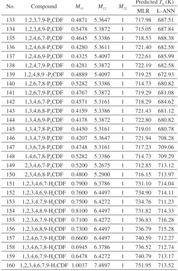
Table 3. Predicted Tb of PCDD/Fs
No. Compound M11 M12 M22
Predicted Tb (K) MLR L-ANN 1 1,2-D2CDD 0.1111 2.1025 0.25 640.94 580.70 2 1,3-D2CDD 0.0625 2.1025 0.25 643.84 619.08 3 1,4-D2CDD 0.0400 2.1250 0.25 645.87 618.27 4 1,6-D2CDD 0.0204 2.1250 0.25 647.04 648.84 5 1,7-D2CDD 0.0156 2.1025 0.25 646.64 655.04 6 1,8-D2CDD 0.0204 2.1025 0.25 646.36 654.83 7 1,9-D2CDD 0.0278 2.1250 0.25 646.60 681.58 8 1,2,3-T3CDD 0.2847 3.1425 0.25 662.30 688.44 9 1,2,6-T3CDD 0.1471 3.1650 0.25 671.19 684.58 10 1,2,7-T3CDD 0.1391 3.1425 0.25 670.99 701.32 11 1,2,8-T3CDD 0.1471 3.1425 0.25 670.51 710.91 12 1,2,9-T3CDD 0.1593 3.1650 0.25 670.47 720.17 13 1,3,6-T3CDD 0.1033 3.1650 0.25 673.81 720.17 14 1,3,8-T3CDD 0.0953 3.1425 0.25 673.60 713.33 15 1,3,9-T3CDD 0.1059 3.1650 0.25 673.65 734.79 16 1,4,6-T3CDD 0.0882 3.1875 0.25 675.40 738.64 17 1,4,7-T3CDD 0.0760 3.1650 0.25 675.44 761.32 18 2,3,6-T3CDD 0.1471 3.1425 0.25 670.51 761.32 19 1,2,3,6-T4CDD 0.3412 4.2050 0.25 691.32 763.27 20 1,2,3,8-T4CDD 0.3331 4.1825 0.25 691.12 764.26 21 1,2,3,9-T4CDD 0.3485 4.2050 0.25 690.89 771.98 22 1,2,4,6-T4CDD 0.2774 4.2275 0.25 695.82 783.51 23 1,2,4,7-T4CDD 0.2620 4.2050 0.25 696.05 803.19 24 1,2,4,8-T4CDD 0.2653 4.2050 0.25 695.85 576.54 25 1,2,4,9-T4CDD 0.2822 4.2275 0.25 695.53 614.90 26 1,2,6,7-T4CDD 0.2862 4.2050 0.25 694.61 614.09 27 1,2,6,8-T4CDD 0.2457 4.2050 0.25 697.02 645.50 28 1,2,6,9-T4CDD 0.2353 4.2275 0.25 698.33 652.00 29 1,2,7,8-T4CDD 0.2829 4.1825 0.25 694.12 651.19 30 1,2,7,9-T4CDD 0.2498 4.2050 0.25 696.78 681.58 31 1,2,8,9-T4CDD 0.3064 4.2050 0.25 693.40 684.22 32 1,3,6,9-T4CDD 0.1867 4.2275 0.25 701.23 685.13 33 1,3,7,9-T4CDD 0.1997 4.2050 0.25 699.77 699.64 34 1,4,6,9-T4CDD 0.1764 4.2500 0.25 702.53 709.01 35 1,4,7,8-T4CDD 0.2232 4.2050 0.25 698.37 711.69 36 1,2,3,4,6-P5CDD 0.5825 5.2675 0.25 709.32 717.36 37 1,2,3,6,7-P5CDD 0.4959 5.2450 0.25 713.81 717.99 38 1,2,3,6,8-P5CDD 0.4520 5.2450 0.25 716.43 710.19 39 1,2,3,6,9-P5CDD 0.4450 5.2675 0.25 717.53 736.39 40 1,2,3,7,9-P5CDD 0.4546 5.2450 0.25 716.27 741.07 41 1,2,3,8,9-P5CDD 0.5080 5.2450 0.25 713.08 735.10 42 1,2,4,6,7-P5CDD 0.4369 5.2675 0.25 718.01 760.64 43 1,2,4,6,8-P5CDD 0.3916 5.2675 0.25 720.72 758.77 44 1,2,4,6,9-P5CDD 0.3860 5.2900 0.25 721.74 759.08 45 1,2,4,7,9-P5CDD 0.3931 5.2675 0.25 720.63 760.07 46 1,2,4,8,9-P5CDD 0.4450 5.2675 0.25 717.53 763.27 47 1,2,3,4,6,7-H6CDD 0.7577 6.3075 0.25 730.58 767.84 48 1,2,3,4,6,8-H6CDD 0.7091 6.3075 0.25 733.48 757.77 49 1,2,3,4,6,9-H6CDD 0.7068 6.3300 0.25 734.31 780.19 50 1,2,3,6,7,9-H6CDD 0.6622 6.3075 0.25 736.28 783.97 51 1,2,3,6,8,9-H6CDD 0.6670 6.3075 0.25 736.00 780.70 52 1,2,4,6,8,9-H6CDD 0.6113 6.3300 0.25 740.01 799.58
No. Compound M11 M12 M22
Table 3. Predicted Tb of PCDD/Fs (cont.)
No. Compound M11 M12 M22
Predicted Tb (K) MLR L-ANN 105 1,2,8,9-T4CDF 0.3382 4.3472 1 695.84 787.51 106 1,3,4,6-T4CDF 0.2896 4.2761 1 696.57 616.67 107 1,3,4,7-T4CDF 0.2701 4.2536 1 697.05 614.90 108 1,3,4,8-T4CDF 0.2774 4.2761 1 697.30 648.04 109 1,3,4,9-T4CDF 0.3018 4.3247 1 697.33 650.28 110 1,3,6,7-T4CDF 0.2578 4.2536 1 697.78 652.51 111 1,3,6,9-T4CDF 0.2111 4.3247 1 702.74 653.28 112 1,3,7,8-T4CDF 0.2530 4.2536 1 698.07 652.92 113 1,4,6,7-T4CDF 0.2475 4.2761 1 699.08 653.28 114 1,4,6,8-T4CDF 0.2062 4.2986 1 702.23 654.28 115 1,4,6,9-T4CDF 0.2033 4.3472 1 703.89 649.34 116 1,4,7,8-T4CDF 0.2401 4.2761 1 699.53 651.53 117 1,6,7,8-T4CDF 0.3607 4.2761 1 692.33 651.49 118 2,3,4,6-T4CDF 0.3607 4.2275 1 690.85 645.50 119 2,3,4,7-T4CDF 0.3364 4.2050 1 691.61 650.67 120 2,3,4,8-T4CDF 0.3412 4.2275 1 692.01 651.53 121 2,3,6,7-T4CDF 0.3017 4.2050 1 693.68 674.69 122 2,3,6,8-T4CDF 0.2578 4.2275 1 696.99 679.98 123 2,4,6,7-T4CDF 0.2652 4.2275 1 696.55 682.91 124 2,4,6,8-T4CDF 0.2214 4.2500 1 699.85 683.34 125 3,4,6,7-T4CDF 0.3064 4.2050 1 693.40 683.38 126 1,2,3,4,6-P5CDF 0.6021 5.3386 1 710.32 683.91 127 1,2,3,4,7-P5CDF 0.5704 5.3161 1 711.53 679.17 128 1,2,3,4,8-P5CDF 0.5826 5.3386 1 711.49 685.63 129 1,2,3,4,9-P5CDF 0.6143 5.3872 1 711.08 685.58 130 1,2,3,6,7-P5CDF 0.5235 5.3161 1 714.33 685.93 131 1,2,3,6,8-P5CDF 0.4870 5.3386 1 717.19 686.61 132 1,2,3,6,9-P5CDF 0.4889 5.3872 1 718.56 687.40
No. Compound M11 M12 M22
Predicted Tb (K) MLR L-ANN 133 1,2,3,7,9-P5CDF 0.4871 5.3647 1 717.98 687.51 134 1,2,3,8,9-P5CDF 0.5478 5.3872 1 715.05 687.84 135 1,2,4,6,7-P5CDF 0.4645 5.3386 1 718.53 688.38 136 1,2,4,6,8-P5CDF 0.4280 5.3611 1 721.40 682.58 137 1,2,4,6,9-P5CDF 0.4325 5.4097 1 722.61 685.99 138 1,2,4,7,9-P5CDF 0.4281 5.3872 1 722.19 682.58 139 1,2,4,8,9 -P5CDF 0.4889 5.4097 1 719.25 672.93 140 1,2,6,7,8-P5CDF 0.5282 5.3386 1 714.73 680.82 141 1,2,6,7,9-P5CDF 0.4767 5.3872 1 719.29 681.08 142 1,3,4,6,7-P5CDF 0.4571 5.3161 1 718.29 684.62 143 1,3,4,6,8-P5CDF 0.4159 5.3386 1 721.43 681.12 144 1,3,4,6,9-P5CDF 0.4178 5.3872 1 722.80 680.82 145 1,3,4,7,8-P5CDF 0.4450 5.3161 1 719.01 680.78 146 1,3,4,7,9-P5CDF 0.4207 5.3647 1 721.94 708.28 147 1,3,6,7,8-P5CDF 0.4748 5.3161 1 717.23 709.06 148 1,4,6,7,8-P5CDF 0.5282 5.3386 1 714.73 709.29 149 2,3,4,6,7-P5CDF 0.5200 5.2675 1 712.85 713.12 150 2,3,4,6,8-P5CDF 0.4800 5.2900 1 716.15 713.97 151 1,2,3,4,6,7-H6CDF 0.7900 6.3786 1 731.10 714.04 152 1,2,3,4,6,9-H6CDF 0.7600 6.4497 1 734.90 714.11 153 1,2,3,4,7,9-H6CDF 0.7500 6.4272 1 734.76 711.23 154 1,2,3,4,8,9-H6CDF 0.8100 6.4497 1 731.82 714.33 155 1,2,3,6,7,9-H6CDF 0.7100 6.4272 1 736.83 716.28 156 1,2,3,6,8,9-H6CDF 0.7300 6.4497 1 736.79 715.28 157 1,2,4,6,7,9-H6CDF 0.6600 6.4497 1 740.59 712.27 158 1,3,4,6,7,8-H6CDF 0.6945 6.3786 1 736.52 712.74 159 1,3,4,6,7,9-H6CDF 0.6478 6.4272 1 740.79 713.17 160 1,2,3,4,6,7,9-H7CDF 1.0037 7.4897 1 751.95 713.52
CONCLUSIONS
The QSPR model for predicting the boiling point of PCDD/ Fs was investigated. The MDEV index was used as structural descriptor of PCDD/Fs. Both MLR model and L-ANN model were developed and investigated. The predictive ability of the developed models was assessed by leave-one-out cross validation and external validation. The validation result indicates that both MLR model and L-ANN model are practicable for predicting the Tb of PCDD/Fs. It is demonstrated that MDEV index of PCDD/Fs
is quantitatively related to the Tb of PCDD/Fs. MDEV index can
be calculated easily. It is easy and convenient to develop the QSPR model for the Tb of PCDD/Fs based on the MDEV index. In addition,
the validation result demonstrates that both MLR and L-ANN are practicable for modeling the quantitative relationship between the MDEV index and Tb of PCDD/Fs. It is reasonable to predict the Tb
of PCDD/Fs by using the established models. Thus, the Tb of each
PCDD/F congener was predicted by using the developed models. The predicted Tb can be used as an estimation of the boiling point
of PCDD/Fs.
ACKNOWLEDGEMENTS
The work was supported by the National Natural Science Foundation of China No. 21305108 and No. 21375105, the Project Supported by Natural Science Basic Research Plan in Shaanxi Province
of China (Program No. 2014JM2039) and the Innovative Research Team of Xi’an Shiyou University (No. 2013QNKYCXTD01).
REFERENCES
1. Kjeller, L.; Jones, K. C.; Ton, A. E. J.; Rappe, C.; Environ. Sci. Technol.
1996, 30, 1398.
2. Moon, M. H.; Kim, H. J.; Kwon, S. Y.; Lee, S. J.; Chang, Y. S.; Lim, H.; Anal. Chem. 2004, 76, 3236.
3. Mclanchlan, M. S.; Sewart, A. P.; Bacon, J. R.; Jones, K. C.; Environ. Sci. Technol.1996, 30, 2567.
4. Atkinson, J. D.; Hung, P. C.; Zhang, Z.; Chang, M. B.; Yan, Z.; Rood, M. J.; Chemosphere2015, 118, 136.
5. Do, L.; Liljelind, P.; Zhang, J.; Haglund, P.; J. Chromatogr. A 2013, 1311, 157.
6. Rordorf, B. F.; Chemosphere 1989, 18, 783.
7. Admire, B.; Lian, B.; Yalkowsky, S. H.; Chemosphere2014, http:// dx.doi.org/10.1016/ j.chemosphere.2014.06.053.
8. Lian, B.; Yalkowsky, S. H.; J. Chem. Thermodyn. 2012, 54, 250. 9. Lian, B.; Yalkowsky, S. H.; Ind. Eng. Chem. Res. 2012, 51,
16750.
10. Junkes, B. da S.; Amboni, R. D. de M. C.; Yunes, R. A.; Heinzen, V. E. F.; J. Braz. Chem. Soc. 2004, 15, 183.
11. Gutman, I.; Tosovic, J.; J. Serb. Chem. Soc.2013, 78, 805.
13. Yin, C. S.; Guo, W. M.; Lin, T.; Liu, S. S.; Fu, R. Q.; Pan, Z. X.; Wang, L. S.; J. Chin. Chem. Soc.2001, 148, 739.
14. Liu, H. H.; Xiao, X.; Qin, J.; Liu, Y. M.; J. Chongqing Inst. Technol. (In Chinese) 2005, 19, 67.
15. Jiao, L.; Wang, X. F.; Bing, S.; Xue, Z. W.; Li, H.; J. Serb. Chem. Soc. (2014), doi:10.2298/ JSC140716087J.
16. Jiao, L.; Xue, Z. W.; Wang, G. F.; Wang, X. F.; Li, H.; Chemom. Intell. Lab. Syst.2014, 137, 91.
17. Jiao, L.; Wang, X. F.; Li, H.; Wang, Y. X.; J. Serb. Chem. Soc.2014, 79, 965.
18. Mackay, D.; Shiu, W. Y.; Ma, K. C.; Lee, S. C.; Physical-Chemical Properties and Environmental Fate for Organic Chemicals, 2nd ed., CRC Press: Boca Raton, 2006.
19. Jiao, L.; Chemosphere 2010, 80, 671.
20. Galão, O. F.; Borsato, D.; Pinto, J. P.; Visentainer, J. V.; Carrão-Panizzi, M. C.; J. Braz. Chem. Soc.2011, 1, 142.
21. Fatemi, M. H.; Chahi, Z. G.; SAR QSAR Environ. Res. 2012, 23, 155. 22. Noorizadeh, H.; Farmany, A.; Noorizadeh, M.; Quim. Nova201134,
242.
23. Nunes, C. A.; Lima, C. F.; Barbosa, L. C. A.; Quim. Nova2011, 34, 279. 24. Fatemi, M.; Ghorbannezhad, Z.; J. Serb. Chem. Soc.2011, 76, 1003. 25. Jiao, L.; Li, H.; Chemom. Intell. Lab. Syst. 2010,103, 90.
26. http://www.statsoft.com/textbook/neural-networks, accessed September, 2014.
27. Zhang, Y. X.; Li, H.; Hou, A. X.; Havel, J.; Chemom. Intell. Lab. Syst.
2006, 82, 165.
28. Yin, C. S.; Shen, Y.; Liu, S. S.; Yin, Q. S.; Guo, W. M.; Pan, Z. X.; Comput. Chem.2001, 25, 239.
29. Zhang, W. J.; Zhong, X. Q.; Liu, G. H.; Stochastic Environmental Re-search and Risk Assessment2008, 22, 207.