On High Order Barycentric Root-Finding Methods
M.M. GRAC¸ A1 and P.M. LIMA2*
Received on July 25, 2016 / Accepted on October 3, 2016
ABSTRACT.To approximate a simple root of a real function f we construct a family of iterative maps, which we callNewton-barycentricfunctions, and analyse their convergence order. The performance of the resulting methods is illustrated by means of numerical examples.
Keywords:order of convergence, Newton’s method, Newton-barycentric map, nonlinear equations.
1 INTRODUCTION
The classical Newton’s iterative scheme for approximating the roots of an equation has been generalized by many authors in order to define iterative maps going from cubical to arbitrary orders of convergence (see for instance [1, 2, 3, 5, 6, 8, 9, 10, 11, 12, 13], and references therein). In particular we mention the third-order method introduced in [13] and a family of high-order methods based on quadrature rules, recently described in [3].
In that work the authors have introduced a recursive algorithm for constructing iterative maps. The first iterative function of this family is the classical Newton’s method, which can be seen as the result of applying the rectangles rule to approximate a certain integral. As it is well-known, Newton’s method has, in general, second order of convergence (when applied to the computation of simple roots). In the referred work [3], the authors have shown that iterative maps of arbitrarily high order can be obtained if quadrature rules of higher degree are used (instead of the rectangles rule) to compute the mentioned integral. The properties of these methods were analysed and their convergence has been illustrated by several numerical examples.
In the present work we also construct a family of high order iterative maps, starting with the Newton’s method, but we follow a different approach. All the iterative mapstto be considered have the common structuret(x)=x−[φ (x)]−1 f(x), where f is a real function with a simple
*Corresponding author: Pedro Miguel Lima.
1Departamento de Matem´atica, Instituto Superior T´ecnico, Universidade de Lisboa, 1049-001 Lisboa, Portugal. E-mail: [email protected]
zero atz. The functionφwill be called amodel function. This model function depends on f and on another functionhwhich we namestep function.
The family of iterative maps to be discussed is constructed by choosing a certain model function φ. We remark that our approach does not follow the traditional path for generating iterative maps by direct or inverse hyperosculatory interpolation (see, for instance [12]) or Taylor expansions around a zero of f (see for instance [10]).
Given a real-valued function f defined on an open setD ⊂R, we assume that f is sufficiently smooth in a neighbourhood of asimple zero zof f. In what follows we show how to construct a family of iterative mapst generating a sequencexi+1=t(xi),i =0,1, . . ., converging locally
toz.
Maps of higher order of convergence can produce accurate approximations with a smaller number of iterations. However, in general, they have expressions of increasing complexity, and so aug-menting its computational cost. In this paper we show that at least for some Newton-barycentric methods the gain in accuracy compensates the computational cost. Like other root-finding meth-ods these iterative maps can be easily extended to the case of multivariate functions. Numerical experiments have been carried out and the results are promising. The corresponding theory is still under construction.
The paper is organized as follows. In Section 2 we introduce the notion of a model functionφ and prove that the iterative mapt(x)=x −[φ (x)]−1 f(x)has a certain order of convergence (see Proposition 2.1). This is the main idea for the construction of recursive families of iterative functions.
In Section 3 we describe in detail one of these families, which we call the Newton-barycentric iterative maps. We begin by specifying the choice of the model function in the case of this family (Subsection 3.1). Then we describe the algorithm for obtaining iterative maps, based on this model function and we give the formulae of some of these maps (Subsection 3.2). In Section 4 we analyse the application of some Newton-barycentric formulas to some numerical examples. We finish in Section 5 with some conclusions.
2 RECURSIVE FAMILIES OF ITERATIVE MAPS
In this section we describe a procedure for constructing recursive families of higher order iterative methods.
Proposition 2.1. Let z be a simple zero of a function f : D ⊂ R → Randφ a sufficiently
smooth function in a neighbourhood of z, such that its derivativesφ(i)satisfy the j+1equalities
φ(i)(z)= f (i+1)(z)
for j ≥ 0 a fixed integer. Then, for any initial value x0 sufficiently close to z, the iterative process xk+1=t(xk), k=0,1, . . ., with
t(x)=x−[φ (x)]−1 f(x), (2.2)
converges to z and its order of convergence is at least j+2.
Proof. From (2.2) it is obvious that the zero z of f is a fixed point of the map t (that is,
t(z)=z). Let us consider the function tdefined by
t(x)=t(x)−x.
Note that its derivatives are
(1)t(x)=t(1)(x)−1, and (i)t(x)=t(i)(x), for i ≥2.
We now use induction on j to prove that the hypotheses in (2.1) imply that t(z) = 0, (1)t(z) = −1,(j)t(z) = 0, for j ≥ 2, and consequentlyt has the referred order of con-vergence.
Let j =0. Rewriting (2.2) as
φ (x) t(x)= −f(x), (2.3)
and applying the derivative operator to this equation, we have
φ(1)(x) t(x)+φ (x) (1)t(x)= −f(1)(x). (2.4)
Sincet(z)=0, andφsatisfies (2.1) withi =0, it follows that f(1)(z) (1)t(z)= −f(1)(z). Aszis a simple zero for f, then
(1)t(z)= −1 ⇐⇒ t(1)(z)=0,
which means that the iterative process generated bythas local order of convergence pat least 2. That is,p≥ j+2.
Let j =1. Differentiating (2.4), we get
φ(2)(x) t(x)+2φ(1)(x) (1)t(x)+φ (x) (2)t(x)= −f(2)(x).
Sincet(z)=0 and(1)t(z)= −1, we obtain
−2 f
(2)(z)
2 + f
(1)(z) (2)t(z)= −f(2)(z).
Therefore(2)t(z)=t(2)(z)=0, and so the iterative process has local order of convergence at least 3= j+2.
For an integerm≥2, assume that
φ(j)(z)= f
(j+1)(z)
and
(1)t(z)= −1, (j)t(z)=0, for j =2,3, . . . ,m. (2.5)
Let us show that(m+1)t(z)=t(m)(z)=0. From (2.3) and the Leibniz’s rule for the derivatives of the product, we have
φ(m+1)(x) t(x)+
m
+1
1
φ(m)(x) (1)t(x)+ · · · +
m
+1
m
φ(1)(x) (m)t(x)
+φ(0)(x) (m+1)t(x)= −f(m+1)(x).
Thus, by the induction hypotheses, we obtain
−
m+
1 1
f(m+1)(z)
m+1 + f
(1)(z) (m+1)t(z)= −f(m+1)(z) ⇔(m+1)t(z)= 0.
Hence the iterative maptm+1has local order of convergence p≥m+2 and the proof is complete.
Remark 2.1. The well-known result on the local order of convergence of the Newton’s map
t(x)=x−f(1)(x)−1 f(x)follows immediately from Proposition 2.1. It is enough to see that (2.1) is verified for j = 0, i.e. φ(0)(z) = f(1)(z), and sot has local order of convergence at least 2.
With the aim of analysing in detail the process of creating iterative maps, proposed in Proposi-tion 2.1, we will now introduce the definiProposi-tions of model funcProposi-tion and step funcProposi-tion.
Definition 2.1.Let z be a simple zero of a function f : D⊂R→R, h andφsufficiently smooth functions in a neighbourhood of z, and j ≥0a fixed integer.
• A functionφ is called a model function of degree j , at x = z, if it satisfies the j +1 conditions(2.1), but does not satisfy a similar condition for i = j+1.
• A function h is called a step function of degree j at x =z (or simply a step function) if it satisfies the following j+1equalities:
h(z)=0, h(1)(z)= −1 and h(i)(z)=0, for i=2,3, . . . ,j, (2.6)
but does not satisfy the condition corresponding to i= j+1.
Example 2.1.Under the conditions of Definition 2.1, set
φ (x)≡ f′(x). (2.7)
Then we haveφ′(z)= f′′(z)butφ′′(z)= f′′′(z)= f′′′(z)/2. Therefore,φdefined by (2.7) is a model function of degree 0.
In the same way, let
h(x)≡φ−1(x)f(x)=f(1) −1
In this case,h(z)= f(z)/f′(z)=0, buth′(z)=1− f(z)f′′(z)/(f′(z))2=1= −1. Henceh defined by (2.8) is a step function of degree 0.
The above defined model functionφand step functionh can be used to define the mapt(x)= x−f(1)(x)−1
f(x), which coincides with the Newton’s method (see Remark 2.1).
3 THE NEWTON-BARYCENTRIC MAPS
We now consider a family of iterative maps, based on the model functionφk, defined as follows:
φk is the inner product of a constant vectorial functionUkand a functionVkdepending only on
the first derivative f(1)evaluated atx+i h(x), fori =0, . . . ,k. Namely, we take
Uk(x)=(a0,a1,a2, . . . ,ak)=a, (3.1)
where the choice ofawill be discussed below, and
Vk(x)=
f(1)(x), f(1)(x+h(x)), . . . , f(1)(x+k h(x)), (3.2)
wherehis a step function of degreek. If one proves thatφk = a,Vk(x)is a model function of
degreekthen, by Proposition 2.1, the respective processtk(x)=x−[φk(x)]−1 f(x)has order
of convergence at leastk+2.
3.1 Choice of the model function
The next proposition shows thatφk is a model function of degreekif and only ifUk(x)=ais
the unique solution of a non homogeneous linear system. Moreover, this solution representsthe barycentric coordinates ofφk in a basis defined by the components of Vk. The name
Newton-barycentric mapsreflects this property, as well as the fact that the recursive process starts with the Newton’s method.
Proposition 3.1. Let f be a function satisfying the hypotheses of Proposition 2.1, h a step
function of degree k, k ≥0a fixed integer andφk = Uk,Vk, with Uk and Vk defined by(3.1)
and(3.2). That is,
φk(x)=a0f(1)(x)+a1f(1)(x+h(x))+ · · · +akf(1)(x+k h(x)). (3.3)
Then, the derivative of order k of Vk, evaluated at x =z, is Vk(k)(z)=DkRk, where Dkand Rk
are the following(k+1)×(k+1)matrices
Dk =diag
f(1)(z), f(2)(z), . . . ,f(k+1)(z)
,
and
Rk = ⎡ ⎢ ⎢ ⎢ ⎢ ⎢ ⎢ ⎣
1 1 1 1 . . . 1
1 0 −1 −2 . . . −(k−1)
1 0 1 22 . . . (k−1)2
..
. ... ... ... ... ...
1 0 (−1)k (−1)k2k . . . (−1)k(k−1)k
Furthermore,
(i) The functionφk is a model function of degree k if and only if
Uk =a=(a0,a1,a2, . . . ,ak)
is the (unique) solution of the linear system
Rka=b, with b=(1,1/2,1/3, . . . ,1/(k+1)) . (3.5)
In particular, this solution satisfies the equality
k
i=0
ai =1. (3.6)
(ii) If f(i)(z) = 0 for i = 1, . . . ,k, then the function Uk = a represents the (normalized)
barycentric coordinates of the model functionφkrelative to the basis,
Vk=f(1)(x), f(1)(x+h(x)), . . . , f(1)(x+k h(x)).
Moreover, the iterative process generated by tk(x)= x−[φk(x)]−1 f(x)has order of
conver-gence at least k+2.
Proof. Fori =0,1, . . . ,kthe derivatives of orderiofVk, evaluated atx=z, are:
Vk(0)= f(1)(z) (1,1,1,1,1, . . . ,1)
Vk(1)= f(2)(z) (1,0,−1,−2,−3, . . . ,−(k−1))
Vk(2)= f(3)(z)
1,0,1,22,32, . . . , (k−1)2
.. .
Vk(k) = f(k+1)(z)1,0, (−1)k, (−1)k2k, (−1)k3k, . . . , (−1)k(k−1)k.
So, the equalities (3.5) hold.
For (i), sinceφk = a,Vk(x), it is straightforward to verify that the conditions (2.1) forφkto be
a model function are equivalent to the system Rka =b. So,Uk =amust be a solution of this
system. As Rkis nonsingular, this is the unique solution. Furthermore, sincezis a simple zero
of f, the equality (3.6) holds because it is just the first equation of the systemRka=b.
For (ii), we need to show that forα=(α0, α1, . . . , αk)∈Rk+1, such that
the only solution isα=0. Differentiating (3.7) and evaluating atx=z, we obtain the homoge-neous linear system
diagf(1)(z), f(2)(z), . . . , f(k+1)(z)
Rkα=0,
which admits only the solutionα=0since both the diagonal matrix and Rkare nonsingular.
The last assertion follows from Proposition 2.1 since by item (i) φk is a model function of
degreek.
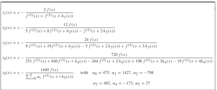
The expressions for the first five barycentric maps are shown in Table 1.
Table 1: First five barycentric type maps.
t1(x)=x−
2f(x)
f(1)(x)+f(1)(x+h
1(x))
t2(x)=x− 12f(x)
5f(1)(x)+8f(1)(x+h
2(x))−f(1)(x+2h2(x))
t3(x)=x− 24f(x)
9f(1)(x)+19f(1)(x+h
3(x))−5f(1)(x+2h3(x))+f(1)(x+3h3(x))
t4(x)=x− 720f(x)
251f(1)(x)+646f(1)(x+h
4(x))−264f(1)(x+2h4(x))+106f(1)(x+3h4(x)−19f(1)(x+4h4(x))
t5(x)=x− 1440f(x) 5
i=0αi f(1)(x+i h5(x))
, with α0=475, α1=1427, α2= −798
α3=482, α4= −173, α5=27
3.2 Construction of the recursive family of iterative maps
We recall that a model functionφdepends on a certain step functionh. Now, for each model function φj included in the definition of the map tj = x −φj(x)−1 f(x), we use a step
function which is defined recursively byhj(x)=tj−1(x)−x. The startert0will be taken to be the Newton’s mapt0(x)= x− [f(1)(x)]−1f(x). The next proposition shows that the iterative maptm, defined recursively in (3.8), has local order of convergence at leastm+2.
Proposition 3.2.Let z be a simple zero of a given function f and t0the Newton’s map
t0(x)=x− [f(1)(x)]−1f(x).
For a given natural number m≥1, define recursively the step function hmand the iterative map
tmby
hj(x)=tj−1(x)−x j=1,2, . . . ,mtj(x)=x−φj(x)−
1
f(x), (3.8)
whereφj is constructed using hj as step function andφj is a barycentric-type map, given by
Proof. It is only necessary to prove that each functionhj is a step function of degree jand the
statement follows from Proposition 3.1.
Let us apply induction on the integerm. Form=1, we haveh1(x)=t0(x)−xand soh1(z)=0 andh(11)(z)= −1.
Letm≥1 be an integer. Ash(m0)(z)=0,hm(1)(z)= −1 and for any integerisuch that 2≤i ≤m,
we haveh(mi)(z)=0, and sohm is a step function of degreem.
The Newton-barycentricmapstk of arbitrary degreek are thus completely defined by
Propo-sition 3.2. Let us remark that the same procedure to construct recursive families of iterative methods can be applied using other types of model and step functions. Moreover the idea of this method is easily extendable to the case of multivariate functions. Multidimensional analogs of the Newton-barycentric maps have been implemented and applied to the solution of systems of nonlinear equations and the numerical results obtained so far are promising.
4 NUMERICAL EXAMPLES
Besides the theoretical interest of this new family of iterative functions, some of the above de-scribed methods are of practical interest. Though they are not optimal in the sense of the Kung and Traub’s conjecture [7], they are more efficient than the Newton’s method, in the sense that with the same number of function evaluations a more accurate result can be produced. Concern-ing for example the Newton’s method (iterative functiont0) and the method with the iterative functiont1, we know that the first one requires 2 function evaluations at each iteration, while the second one requires 3. This means that two iterations of the second method require as many function evalutions (6) as three iterations of the first one. However the result produced by two iterations of the second method is in general much more accurate than the one produced by 3 iterations of the Newton’s method. This happens, because the second method has at least con-vergence order three, and it follows that t1◦t1(the composition oft1 with itself) has at least convergence order 9; on the other hand, since the Newton method has in general convergence order 2, the methodt0◦t0◦t0has just convergence order 8. Concerning the methodt2(fourth order of convergence) each iteration requires 5 function evaluations; however as we shall see in the examples below, one single iteration of this method is often sufficient to obtain a result with an error less than 10−10(which can only be obtained with three iterates of the Newton’s method).
in Tables 2, 3, 4 and they illustrate the advantage of using the methods with the iterative functions t1andt2for approximating the roots of real functions.
Table 2: f(x) = x3 + 4x2 − 10, the initial approximation is x0 = 1, the solution is z=1.3652300134141, with 12 significant digits (see this example in [13]).
Iterative function Error Number of iterations Number of function evaluations
t0 2.13×10⁻¹¹ 3 6
t1 −4.54×10⁻¹⁷ 2 6
t2 −4.54×10⁻¹¹ 1 5
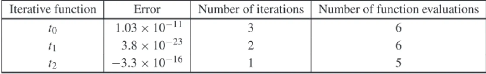
Table 3: f(x) = cos(x) − x, the initial approximation is x0 = 0.1, the solution is z=0.739085133215, with 12 significant digits.
Iterative function Error Number of iterations Number of function evaluations
t0 1.03×10⁻¹¹ 3 6
t1 3.8×10⁻²³ 2 6
t2 −3.3×10⁻¹⁶ 1 5
Table 4: f(x)=tanh(x−1), the initial approximation isx0=0, the exact solution isz=1.
Iterative function Error Number of iterations Number of function evaluations
t0 2.3×10⁻¹³ 4 8
t1 1.8×10⁻¹³ 3 9
t2 4.8×10⁻¹⁹ 2 10
5 CONCLUSIONS
In this work we have introduced a family of high order iterative methods for the numerical so-lution of nonlinear equations. This family starts with the Newton’s method as the basis of the recurrence process. Then each member of the family is build by a well defined procedure, form-ing a sequence of increasform-ing convergence order.
The numerical examples presented in Section 4 demonstrate that the first iterative functions of these family (in particulart1and t2) offer a good alternative to the Newton’s method, taking account their accuracy and number of function evaluations. We remark that these methods can be easily combined with algorithms for the separation of real roots, such as recently described in [4], providing an effective tool for detection and computation of real roots.
ACKNOWLEDGMENTS
RESUMO.Com o fim de aproximar uma raiz simples de uma func¸˜ao realf, constr´oi-se uma
fam´ılia de aplicac¸˜oes iteradoras, que se designam func¸˜oes Newton-baricˆentricas, e
analisa-se a sua ordem de convergˆencia. O deanalisa-sempenho dos m´etodos computacionais resultantes ´e
ilustrado atrav´es de exemplos num´ericos.
Palavras-chave:Ordem de convergˆencia, m´etodo de Newton, func¸˜ao Newton-baricˆentrica,
equac¸˜oes n˜ao-lineares.
REFERENCES
[1] L. Collatz. Functional Analysis and Numerical Mathematics.Academic Press, New York (1966).
[2] A. Cordero & J. Torregrosa. Variants of Newton’s method using fifth-order quadrature formulas.
Appl. Math. Comput.,190(2007), 686–698.
[3] M. M. Grac¸a & P. M. Lima. Root finding by high order iterative methods based on quadratures.
Appl. Math. Comput.,264(2015), 466–482.
[4] M. M. Grac¸a. Maps for global separation of roots.Electronic Transactions on Numerical Analysis,45 (2016), 241–256.
[5] Y. Ham, C. Chun & S.–G. Lee. Some higher-order modifications of Newton’s method for solving nonlinear equations.J. Comp. Appl. Math.,222(2008), 477–486.
[6] A. S. Householder. The Numerical Treatment of a Single Nonlinear Equation.McGraw-Hill, New York (1970).
[7] H. T. Kung & J. F. Traub. Optimal order of one-point and multipoint iteration.J. Assot. Comput. Math.,21(1974), 634–651.
[8] G. Labelle. On extensions of the Newton-Raphson iterative scheme to arbitrary orders.Disc. Math Th. Comput Sc. (DMTCS), proc. AN, 845–856, Nancy, France (2010).
[9] W. C. Rheinboldt. Methods for Solving Systems of Nonlinear Equations. 2nd Ed.,SIAM, Philadelphia (1998).
[10] P. Sebah & X. Gourdon. Newton’s method and high order iterations, 2001. Available from: http://numbers. computation.free.fr/Constants/constants.html.
[11] G. Fernandez-Torres. Derivative free iterative methods with memory of arbitrary high convergence order.Numer. Alg.,67(2014), 565–580.
[12] J. F. Traub. Iterative Methods for the Solution of Equations.Prentice-Hall, Englewood Cliffs (1964).
[13] S. Weerakoon & G. I. Fernando. A variant of Newton’s method with accelerated third-order conver-gence.App. Math. Lett.,13(2000), 87–93.