ISSN 0101-8205 www.scielo.br/cam
A one-shot inpainting algorithm based on the
topological asymptotic analysis
DIDIER AUROUX∗ and MOHAMED MASMOUDI
Laboratoire MIP, Université Paul Sabatier Toulouse 3, 31062 Toulouse cedex 9, France
∗E-mail: [email protected]
Abstract. The aim of this article is to propose a new method for the inpainting problem.
Inpainting is the problem of filling-in holes in images. We consider in this article the crack
localization problem, which can be solved using the Dirichlet to Neumann approach and the
topological gradient. In a similar way, we can define a Dirichlet and a Neumann inpainting
problem. We then define a cost function measuring the discrepancy between the two corresponding
solutions. The minimization is done using the topological asymptotic analysis, and is performed
in only one iteration. The optimal solution provides the best localization of the missing edges,
and it is then easy to inpaint the holes.
Mathematical subject classification: 68U10, 94A08, 34E05.
Key words:image inpainting, topological asymptotic analysis, inverse conductivity problem.
1 Introduction
The inverse conductivity problem, the so called Calderon problem [12], consists in identifying the coefficients of a partial differential equation from the knowl-edge of the Dirichlet to Neumann operator. This problem has been widely studied in literature [15, 16, 23, 24].
In the particular case of cracks identification, the problem seems to be more convenient to solve thanks to the singularities of the solution. Only two mea-surements are needed to recover several simple cracks [2, 7, 3].
From the numerical point of view, several methods [3, 4, 8, 9, 10, 11, 15, 26, 28] have been proposed.
We don’t know if these methods are considered in real life applications outside laboratories, so we are proposing in this paper an unexpected real application of crack detection: the inpainting problem.
The goal of inpainting is to fill a hidden part of an image. In other words, if we denote bythe original image andωthe hidden part of the image, our goal is to recover the hidden part from the known part of the image in\ω. This problem has been widely studied. Mainly two methods have been considered:
• Extrapolation approach, the image is approximated in\ω, then the ap-proximate function is evaluated inω[31, 32],
• Minimization of an energy cost function inω based on a total variation norm [13, 14].
Crack detection allows to identify the edges of the hidden part of the image, the inpainting problem is then solved easily. Our crack detection technique [3] is based on the topological gradient approach [17, 20, 19, 25, 27, 29, 30].
Similar ideas have been applied by the authors to image restoration and clas-sification [6, 21, 5].
This papers is organized as follows. In section 2, we recall our method for crack localization. In section 3, we present the adaptation of this technique to inpainting. Our crack localization technique gives satisfying results with incomplete data [21]; in section 4, we show that we are able to recover the image inωwhen the intersection of its boundary with the boundary ofis not empty. We end the paper with some concluding remarks in section 5.
2 Crack localization problem
2.1 Dirichlet and Neumann problems
fluxφ ∈ H−1/2(Ŵ)on the boundaryŴof, and we want to findσ ⊂ such that the solutionu ∈ H1(\σ )to
1u=0 in\σ, ∂nu=φ onŴ,
∂nu=0 onσ,
(1)
satisfiesu|Ŵ = T where T is a given function of H1/2(Ŵ). In order to have a
well-posed problem, we assume that
Z
Ŵ
φds =0. (2)
As we have an over-determination in the boundary conditions, we can define aDirichletand aNeumannproblem:
FinduD ∈ H1(\σ )such that
1uD =0 in\σ,
uD =T onŴ,
∂nuD =0 onσ,
(3)
and
finduN ∈ H1(\σ )such that
1uN =0 in\σ,
∂nuN =φ onŴ,
∂nuN =0 onσ.
(4)
It is clear that for the unknown crack σ∗, the two solutions uD anduN are
equal. The idea is then to consider the following cost function:
J(σ )= 1
2kuD−uNk 2
L2(), (5)
whereuDanduNare solutions to problems(3)and(4)respectively for the given
crackσ.
2.2 Minimization by topological asymptotic analysis
We consider in this section the two corresponding adjoint states, respectively solutions inH1()to
(
−1vD = −(uD−uN) in,
vD =0 onŴ,
and
(
−1vN = +(uD−uN) in,
∂nvN =0 onŴ.
(7)
The cost function J(0)corresponds to the value of the cost function when no crack is inserted in the domain. In the following, we denote byσ a fixed bounded crack containing the origin O, and byn a unit vector normal to this crak. We consider the insertion of a small crack at pointx: σ =x+εσ, where εis supposed to be small.
The variation of the cost function induced by the insertion of this small crack is J(σ )−J(0), and the topological gradient theory provides the following asymp-totic expansion ofJ whenεtends to zero [3]:
J(σ )−J(0) = f(ε)g(x,n)+o(f(ε)), (8)
where f is a positive function depending only on the size of the crack, satisfying lim
ε→0 f(ε) = 0, and where g is called the topological gradient, depending only on the location of the inserted crack. The insertion of small cracks whereg is negative will hence minimize the cost function.
The topological gradient associated to the cost function J defined in(5) is given by
g(x,n) = −(∇uD(x).n)(∇vD(x).n)+(∇uN(x).n)(∇vN(x).n)
. (9)
The topological gradient can then be rewritten in the following way
g(x,n) = nTM(x)n, (10)
whereM(x)is the 2×2 symmetric matrix defined by
M(x) = −sym ∇uD(x)⊗ ∇vD(x)+ ∇uN(x)⊗ ∇vN(x)
. (11)
We can deduce that g(x,n) is minimal when the normaln is the eigenvector associated to the smallest (i.e. most negative) eigenvalue of the matrixM(x). In the following, this eigenvalue will be considered as the topological gradient.
adjoint problems. Then, at each pointx of the domain, we compute the matrix M(x)and its two eigenvalues. The crack likely lies in the most negative gradient regions.
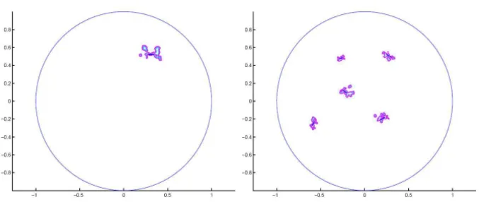
Applying the procedure described above, an example of location of the un-known cracks using the topological gradient is shown on figure 1 (extracted from [3]). The most negative values of the topological gradient are located around the actual cracks, and these results are obtained in only one iteration.
Figure 1 – Left: actual cracks; right: superposition of the actual cracks and a topological
gradient isovalue. Figure extracted from [3].
3 Application to inpainting problems
3.1 Algorithm
We denote bythe image andŴits boundary,ωthe missing part of the image andγ its boundary. vrepresents the image we want to restore,T will represent here the value of the image on the boudary of the missing zone, andφ will be the corresponding flux. We have thenT =vandφ =∂nvin the corresponding
domains. Theoretically, we have to assumevto be enough regular, for example inH2(), but it will be possible to work withvinL2().
We now consider the problem of findinguα ∈ H1(), solution to the following
equation:
(
−α1uα +uα.χ\ω =v.χ\ω in,
∂nuα =0 onŴ,
whereαis a small positive number. This equation can be rewritten as
finduα ∈ H1()such that
−α1uα+uα =v in\ω,
1uα =0 inω,
∂nuα =0 onŴ.
(13)
Whenα → 0, it is morally equivalent whenvis regular to find the solution uN ∈ H1(\γ )to
uN =v in\ω,
1uN =0 inω,
∂nuN =∂nv onγ ,
(14)
which can be seen as a Neumann problem.
From a numerical point of view, we will solve equation(13)with a very small positiveα and we will consider that it is ourNeumannproblem. The Dirichlet problem does not require any special care.
The inpainting algorithm is then the following:
• Calculation ofuDanduN, respectively solutions to
uD =v in\ω,
1uD =0 inω,
uD =v onγ ,
(15)
whereuD ∈ H1(), and
−α1uN+uN =v in\ω,
1uN =0 inω,
∂nuN =0 onŴ,
(16)
whereuN is inH1()(the normal derivative is the same on the two sides
ofγ).
• Calculation ofvDandvNthe two corresponding adjoint states, respectively
solutions to
vD =0 in\ω,
−1vD = −(uD−uN) inω,
vD =0 onγ ,
and
vN =0 in\ω,
−1vN = +(uD−uN) inω,
∂nvN =0 onγ .
(18)
• Computation of the 2× 2 matrix M(x) (see eq. (11)) and its lowest eigenvalueλmi n at each point of the missing domainω.
• Definition of cracks localization: {x ∈ω; λmi n(x) < δ <0}, whereδis
a negative threshold.
• Calculation ofusolution to the Neumann problem(4)with this crackσ.
This algorithm has a complexity of O(n.log(n)), where n is the size of the
image (i.e. number of pixels). See [5] for more details.
3.2 Numerical results
3.2.1 Synthetic images
We first consider a synthetic image, consisting of a black square on a white background. We assume that the center of the image is occluded. The missing region is represented by the grey square on image 2-a. A very fast approach for filling in the hole consists of solving the Laplace equation in the hole, with a Dirichlet boundary condition, i.e. the Dirichlet problem defined by equation (15). The corresponding solution is represented in figure 2-b.
We have then applied the algorithm defined in section 3.1, and figures 2-c and 2-d represent the identified cracks (or missing edges of the image) and the corresponding inpainted image respectively. We can notice that the corner of the black square is nearly identified.
5 10 15 20 25 30 35 40 45 50 5
10
15
20
25
30
35
40
45
50
5 10 15 20 25 30 35 40 45 50 5
10
15
20
25
30
35
40
45
50
(a) (b)
5 10 15 20 25 30 35 40 45 5
10
15
20
25
30
35
40
45
5 10 15 20 25 30 35 40 45 50 5
10
15
20
25
30
35
40
45
50
(c) (d)
Figure 2 – Inpainting of a black square on a white background: occluded image (a), Laplace filled-in image (b), topological gradient (c) and inpainted image (d).
the holeω and the image\ω, and hence the local geometry of the image is restored.
3.2.2 Real images
We have then applied our algorithm to the inpainting of a real image. Figure 4 shows respectively the image occluded by a black square (a), the filled-in image using the Laplace operator (b), the identified missing edges (c) and the corresponding inpainted image (d).
5 10 15 20 25 30 35 40 45 50 5
10
15
20
25
30
35
40
45
50
5 10 15 20 25 30 35 40 45 50 5
10
15
20
25
30
35
40
45
50
(a) (b)
5 10 15 20 25 30 35 40 45 5
10
15
20
25
30
35
40
45
5 10 15 20 25 30 35 40 45 50 5
10
15
20
25
30
35
40
45
50
(c) (d)
Figure 3 – Inpainting of a black circle on a white background: occluded image (a),
Laplace filled-in image (b), topological gradient (c) and inpainted image (d).
on the domainrepresenting the image.
We now consider the occlusion of the same image by a black thick line. Figure 6 represents the results of our algorithm, and figure 7 represents a zoom of the same images. One can see that the image is still very well inpainted, even if the missing part is quite large. We may remark that we used the same thresholdδ(see the algorithm in the previous section) for this whole zone, and it could be more interesting to look for valley lines of the topological gradient.
4 Boundary inpainting
50 100 150 200 250 50
100
150
200
250
50 100 150 200 250 50
100
150
200
250
(a) (b)
50 100 150 200 250 50
100
150
200
250
50 100 150 200 250 50
100
150
200
250
(c) (d)
Figure 4 – Inpainting of a black square on a real image: occluded image (a), Laplace filled-in image (b), topological gradient (c) and inpainted image (d).
4.1 Crack localization using incomplete data
In comparison with section 2.1, we can assume that the input flux φ is still imposed on the whole boundary Ŵ of , whereas the Dirichlet condition is incomplete: we assume that we measureuon only a partŴ0of the boundaryŴ. We denote byŴ1the complementary set in the boundary ofŴ0: Ŵ=Ŵ0∪Ŵ1.
We can still solve the Neumann problem:
1uN =0 in\σ,
∂nuN =φ onŴ,
∂nuN =0 onσ,
(19)
95 100 105 110 115 120 125 20
25
30
35
40
45
95 100 105 110 115 120 125 15
20
25
30
35
40
45
50
(a) (b)
90 95 100 105 110 115 120 125 130 15
20
25
30
35
40
45
50
95 100 105 110 115 120 125 15
20
25
30
35
40
45
50
(c) (d)
Figure 5 – Inpainting of a black square on a real image: zoom of occluded image (a),
Laplace filled-in image (b), topological gradient (c) and inpainted image (d).
is replaced by the followingDirichlet-Neumannproblem:
1uD =0 in\σ,
uD =T onŴ0, ∂nuD =0 onŴ1, ∂nuD =0 onσ.
(20)
We still consider the same cost function, measuring the discrepancy between these two solutions. The topological gradient remains unchanged, as well as the algorithm defined at the end of section 2.2.
50 100 150 200 250 50
100
150
200
250
50 100 150 200 250 50
100
150
200
250
(a) (b)
50 100 150 200 250 50
100
150
200
250
50 100 150 200 250 50
100
150
200
250
(c) (d)
Figure 6 – Inpainting of a black line on a real image: occluded image (a), Laplace filled-in image (b), topological gradient (c) and inpainted image (d).
is the left half of the boundary, andŴ1is the right half of the boundary. The most negative values of the topological gradient are still located around the actual cracks.
4.2 Boundary inpainting problem
40 50 60 70 80 90 100 20 30 40 50 60 70 80
30 40 50 60 70 80 90 100 20 30 40 50 60 70 80 90 (a) (b)
40 50 60 70 80 90 100 20 30 40 50 60 70 80 90
40 50 60 70 80 90 100 20 30 40 50 60 70 80 90 (c) (d)
Figure 7 – Inpainting of a black line on a real image: zoom of occluded image (a), Laplace filled-in image (b), topological gradient (c) and inpainted image (d).
uD =v in\ω,
1uD =0 inω,
uD =v onγ0, ∂nuD =0 onγ1,
(21) and
−α1uN +uN =v in\ω,
1uN =0 inω,
∂nuN =0 onŴ,
(22)
Figure 8 – Superposition of the actual cracks and a topological gradient isovalue with incomplete data. Figure extracted from [3].
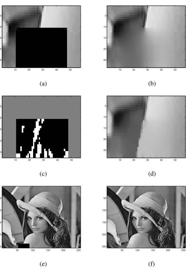
The algorithm is then the same as in the previous section. We have then tried to fill in a real image occluded by a black square box located on the side of the image.
Figures 9-a,b,c,d represent respectively zooms of the occluded image, the Laplace filled-in image, the identified missing edges by the topological gra-dient, and the inpainted image. Figures 9-e and f represent the full size original and inpainted images. We can see that the results are almost the same as in the case of an occlusion inside the image: the missing edges are identified in only one iteration of the topological gradient, and the image is filled-in using only 5 resolutions of a PDE on the image.
5 Conclusion
The crack detection technique, based on topological gradient, provides an excel-lent frame for solving image processing problem. It has been applied to image restoration, image classification and image inpainting.
In all these cases, we obtained excellent results and the computing time is very short. OnlyO(nlog(n))operations are needed to solve the image processing
10 20 30 40 50 5
10
15
20
25
10 20 30 40 50 5
10
15
20
25
(a) (b)
10 20 30 40 50
5
10
15
20
25
10 20 30 40 50 5
10
15
20
25
(c) (d)
50 100 150 200 250 50
100
150
200
250
50 100 150 200 250 50
100
150
200
250
(e) (f)
Figure 9 – Inpainting of a black square on the side of a real image: zoom occluded
REFERENCES
[1] G. Alessandrini, E. Beretta and S. Vessela,Determining linear cracks by boundary measure-ments: Lipschitz stability, SIAM J. Math. Anal.,27(2) (1996), pp. 361–375.
[2] G. Alessandrini and A. Diaz Valenzuela,Unique determination of multiple cracks by two measurements, SIAM J. Control Optim.,34(3) (1996), pp. 913–921.
[3] S. Amstutz, I. Horchani and M. Masmoudi,Crack detection by the topological gradient method, Control and Cybernetics,34(1) (2005), pp. 119-138.
[4] S. Andrieux and A. Ben Abda,Identification of planar cracks by complete overdetermined data: inversion formulae, Inverse Problems,12(1996), pp. 553-563.
[5] D. Auroux, M. Masmoudi and L. Belaid,Image restoration and classification by topological asymptotic expansion, in Variational Formulations in Mechanics: Theory and Applications, E. Taroco, E.A. de Souza Neto and A.A. Novotny (Eds), CIMNE, Barcelona, Spain, in press (2006).
[6] L. Belaid, M. Jaoua, M. Masmoudi and L. Siala,Image restoration and edge detection by topological asymptotic expansion, C.R. Acad. Sci., Ser. I,342(5) (2006), pp. 313–318.
[7] Z. Belhachmi and D. Bucur,Stability and uniqueness for the crack identification problem, SIAM J. Control Optim., to appear.
[8] A. Ben Abda, H. Ben Ameur and M. Jaoua,Identification of 2D cracks by elastic boundary measurements, Inverse Problems,15(1999), pp. 67–77.
[9] A. Ben Abda, M. Kallel, J. Leblond and J.-P. Marmorat,Line-segment cracks recovery from incomplete boundary data, Inverse Problems,18(2002), pp. 1057–1077.
[10] M. Bruhl, M. Hanke and M. Pidcock,Crack detection using electrostatic measurements, Math. Model. Numer. Anal.,35(2001), pp. 595–605.
[11] K. Bryan and M.S. Vogelius,A review of selected works on crack identification, Proceedings of the IMA workshop on Geometric Methods in Inverse Problems and PDE Control, August 2001.
[12] A.P. Calderón,On an inverse boundary value problem, Seminar on Numerical Analysis and Its Applications to Continuum Physics (Rio de Janeiro, 1980), Soc. Brasil. Mat., Rio de Janeiro (1980), pp. 65–73.
[13] T. Chan and J. Shen,Mathematical Models for Local Deterministic Inpaintings, UCLA CAM Tech. Report 00-11, March (2000).
[14] T. Chan and J. Shen,Non-texture Inpainting by Curvature-driven Diffusions (CCD), UCLA CAM Tech. Report 00-35, Sept. (2000).
[15] A. Friedman and M.S. Vogelius,Determining cracks by boundary measurements, Indiana Univ. Math. J.,38(3) (1989), pp. 527–556.
con-ductivity by boundary measurements: a theorem of continuous dependence, Arch. Rational Mech. Anal.,105(4) (1989), pp. 299–326.
[17] S. Garreau, Ph. Guillaume and M. Masmoudi,The topological asymptotic for PDE systems: the elasticity case, SIAM J. Control. Optim.,39(6) (2001), pp. 1756–1778.
[18] J. Giroire and J.-C. Nédélec,Numerical solution of an exterior Neumann problem using a double layer potentiel, Mathematics of computation,32(144) (1978), pp. 973–990.
[19] Ph. Guillaume and K. Sididris,Topological sensitivity and shape optimization for the Stokes equations, MIP Tech. Report 01-24, (2001).
[20] Ph. Guillaume and K. Sididris,The topological asymptotic expansion for the Dirichlet problem, SIAM J. Control Optim.,41(4) (2002), pp. 1052–1072.
[21] L. Jaafar Belaid, M. Jaoua, M. Masmoudi and L. Siala,Application of the topological gradient to image restoration and edge detection, J. of Boundary Element Methods, to appear.
[22] A. Khludnev and V. Kovtunenko,Analysis of cracks in solids, WIT Press, Southampton-Boston, 2000.
[23] R. Kohn and M. Vogelius,Relaxation of a variational method for impedance computed tomography, Comm. Pure Appl. Math.,40(6) (1987), pp. 745–777.
[24] S. Kubo and K. Ohji,Inverse problems and the electric potential computed tomography method as one of their application, in Mechanical Modeling of New Electromagnetic Mate-rials, Elsevier Science Publisher, 1990.
[25] M. Masmoudi,The Topological Asymptotic, in Computational Methods for Control Appli-cations, International Series GAKUTO, 2002.
[26] N. Nishimura and S. Kobayashi,A boundary integral equation method for an inverse problem related to crack detection, Int. J. Num. Methods Engrg.,32(1991), pp. 1371–1387.
[27] B. Samet, S. Amstutz and M. Masmoudi,The topological asymptotic for the Helmholtz equation, SIAM J. Control. Optim.,42(5) (2003), pp. 1523–1544.
[28] F. Santosa and M. Vogelius,A computational algorithm to determine cracks from electrostatic boundary measurements, Int. J. Eng. Sci.,29(1991), pp. 917–937.
[29] A. Schumacher,Topologieoptimisierung von Bauteilstrukturen unter Verwendung von Lopch-positionierungkrieterien, Thesis, Universitat-Gesamthochschule-Siegen, 1995.
[30] J. Sokolowski and A. Zochowski,On the topological derivative in shape optimization, SIAM J. Control Optim.,37(1999), pp. 1241–1272.
[31] P. Wen, X. Wu and C. Wu,An Interactive Image Inpainting Method Based on RBF Networks, J. Wang et al. (Eds.), LNCS 3972, pp. 629–637, 2006.