Josué Labaki
labaki@fem.unicamp.br University of Campinas School of Mechanical Engineering Department of Computational Mechanics 13083-970 Campinas, SP, BrazilLuiz Otávio Saraiva Ferreira
lotavio@fem.unicamp.br University of Campinas School of Mechanical Engineering Department of Computational Mechanics 13083-970 Campinas, SP, BrazilEuclides Mesquita
euclides@fem.unicamp.br University of Campinas School of Mechanical Engineering Department of Computational Mechanics 13083-970 Campinas, SP, BrazilConstant Boundary Elements on
Graphics Hardware: a GPU-CPU
Complementary Implementation
Numerical simulation of engineering problems has reached such a large scale that the use of a parallel computing approach is required to obtain solutions within a reasonable time. Recent efforts have been made to implement these large scale computational tasks on general-purpose programmable graphics hardware (GPGPU). The Graphics Processing Unit (GPU) is specially well-suited to address problems that can be formulated in form of data-parallel computations with high arithmetic intensity. This work addresses the implementation of the direct version of the Boundary Element Method (DBEM) on a complementary GPU-CPU system. In this article, constant elements were used for the solution of 2D potential problems. A serial implementation of the BEM was rewritten under the SIMT (Single Instruction Multiple Thread) parallel programming paradigm. The code was developed on an NVidia CUDA programming environment. The efficiency of the implemented strategies is investigated by solving a representative 2D potential problem. The paper reviews in detail the classical BEM formulation in order to be able to address the possible parallelization steps in the numerical implementation. The article reports the performance of the GPU-CPU system compared to the classical CPU-based system for an increasing number of boundary elements.
Keywords: boundary element method, graphics hardware, high-performance computing, GPU-CPU systems
Introduction1
General Purpose Graphics Processing Units (GPGPU) have been largely investigated in the last years for the high performance computing of Finite Difference Methods, Particle-Based Methods, Lattice-Boltzmann Method, Finite Element Method and also to the Boundary Element Method (Owens et al., 2007). Low-level, graphics-dedicated APIs (Application Programming Interfaces) such as Cg, OpenGL (Schreiner et al., 2005) and DirectX (Jones, 2004) were employed by Takahashi (2006) and Oishi and Yoshimura (2008) for their implementation of the Boundary Element Method and Finite Element Method on the GPU.
A new technology of graphic devices was introduced by the end of 2006, the architecture of which allows them to perform non-graphic data processing. A new API called CUDA (Compute Unified Device Architecture) was launched by NVidia Corporation for this new generation of GPUs (CUDA, 2010). CUDA allows the programmer to code the GPGPU in a higher level paradigm, compared to the former graphics-dedicated APIs such as OpenGL and DirectX (Owens et al., 2007; CUDA, 2010).
Graphics hardware is a very efficient parallel computation device. They resemble non-graphic many-core clusters of ordinary CPUs, but possessing unusually high-bandwidth memories and fast floating-point operations. These features make the GPU an attractive alternative for the implementation of expensive computational tasks. Methods of discretization, such as the Boundary Element Method (BEM), whose parallel formulations have already been explored for CPU clusters (Beer, Smith and Duenser, 2008), are good examples of such expensive computational tasks.
In the process of solution of a problem by the BEM, several non-recursive numerical calculations have to be performed, which are good candidates to parallelization on graphics hardware. Many numerical integrations have to be done, a dense linear system has to be built and solved, and some rectangular and square matrix-vector multiplications have to be performed.
This work addresses the implementation of the Boundary Element Method for two-dimensional potential problems on
Paper received 22 February 2011. Paper accepted 24 August 2011. Technical Editor: Fernando Rochinha
graphics hardware within the CUDA programming environment. The final dense, non-symmetric system of algebraic equations is solved in serial execution on the CPU, which characterizes the present code as a complementary GPU-CPU implementation. The paper begins recalling the classical formulation and serial implementation of the method. Next, the new technology of GPGPU is described in some details. The structure of a GPU, as visible from the CUDA programming environment, is briefly summarized in order to formulate the possible strategies for parallel implementation on the graphics card. It is described why the GPU-CPU implementation is more efficient than its CPU-only counterpart and how the coding of non-graphical algorithms is treated. The fourth section shows how the BEM implementation was approached in order to comply with the GPGPU philosophy. Finally, the presented implementation is used to solve a simple, but representative potential problem with closed-form solution. Its performance is compared with an ordinary CPU serial code for an increasing number of boundary elements.
Nomenclature
A = matrix containing mixed influence terms B = matrix containing mixed influence terms b’ = vector of boundary conditions
D = influence matrix of the internal points G = influence matrix
H = influence matrix h = interpolation function n = normal vector q = normal flux
q = vector of flux quantities
R = distance from the source point to the collocation point S = influence matrix of the internal points
u = potential quantity
u = vector of potential quantities x = position; vector of unkown quantities x0 = collocation point
Greek Symbols
Γ = boundary δ = Dirac’s delta
Subscripts
b = bounded
∞ = unbounded
bu = boundary with prescribed Dirichlet boundary conditions bq = boundary with prescribed Neumann boundary conditions
e = respective to the element The Boundary Element Method
BEM is part of the group of numerical methods which involve some discretization. As it is well-known, the solution of problems by BEM can be divided into the following main steps:
(a) the transformation of the differential equation into a boundary integral equation by a reciprocity relation or by a vector identity;
(b) the discretization of the domain boundary by elements; (c) the calculation of the matrices of influence coefficients by means of integration over the boundary elements;
(d) the incorporation of boundary conditions in terms of nodal values;
(e) the numerical solution of a fully populated algebraic system of equations, furnishing as a result all unknown boundary data;
(f) the determination of the solution within the domain of the problem by integration procedures weighted by the boundary data.
Formulation of BEM for potential problems
Consider a domain Ωb, shown in Fig. 1a, enclosed by a
boundary Γb= Γbu∪Γbq, in which the behavior of a scalar quantity
u(x) is described by the Laplace homogeneous equation, Eq. (1).
( )
20
u
∇ x = (1)
On the portion of the boundary indicated as Γbu, Dirichlet
boundary conditions u(x∈Γbu)=u are prescribed. On the
complementary boundary Γbq Neumann boundary conditions are
given, ∂u(x∈Γbq)/∂n = q. The quantity n indicates the unit vector
normal to the boundary.
Consider also two distinct solutions of the Laplace operator. The first u(x) is the actual solution of the problem being solved. The second solution u*(x, x0) is an auxiliary state that describes the
solution of the Laplace operator at point x for an unbounded domain
Ω∞, shown in Fig. 1b, presenting a Dirac’s Delta source applied at
point x0:
2 *
0 0
( , ) ( )
u δ
∇ x x = − x (2)
a) actual bounded domain ΩΩΩΩb b) auxiliary unbounded domain ΩΩΩΩ∞
Figure 1. Definitions for BEM.
This particular auxiliary solution u*(x, x0) is called fundamental
solution and plays a fundamental role in the formulation of the
Boundary Element Method. A reciprocity relation may be established between these two solutions by applying Green’s Second Identity, leading to (Kane, 1994):
(
)
( ) ( )
(
)
(
)
(
) ( )
( ) (
)
( )
* 2 2 *
* * , , , , b b b
u u u u d
u u
u u d
Ω
Γ
∇ − ∇ Ω
∂ ∂
= − Γ
∂ ∂
∫
∫
0 0 0 0x x x x x x
x x x
x x x x
n n
(3)
In Eq. (3), the normal flux, or the derivative of the solution u*(x,
x0) with respect to the boundary normal n, is also present:
* * 0 0 ( , ) ( , ) u q ∂ = ∂ x x x x n (4)
Using the properties of the Dirac’s Delta, and taking the source point x0 to the boundary Γb, an integral equation, known as
Somigliana identity, may be established relating the boundary values, u(x) and q(x), x ∈Γb, of the actual problem (Kane, 1994):
*
* 0
0 0 0
( ) ( , ) ( ) ( ) ( , ) ( )
b
u u
C u u u d
Γ
∂ ∂
= − Γ
∂ ∂
∫
x x xx x x x x
n n (5)
The integration free term C(x0) is obtained as the result from a
limiting analysis when the collocation point x0 approaches the
boundary Γb (Kane, 1994). It depends fundamentally on the
geometry of the boundary Γb. Equation (5) forms the basis of the
classical BEM formulation for potential problems and it is an exact Boundary Integral Equation in which line integrals must be evaluated along the boundary Γb. For the 2D Laplace operator given
in Eq. (2), the fundamental solution is u*(x,x0) = −ln(R)/2π, with R
being the distance from the field point x to the collocation point x0,
R =x−x0|, (Kane, 1994).
Serial implementation of BEM using constant elements
The formulation of the BEM consists in the discretization of the exact boundary integral expression given by Eq. (5). According to this method, the boundary Γb is discretized in boundary elements Γe,
Γb=ΣΓe, each one having normal vectors ne pointing outward the
domain. The solution over the boundary elements is assumed to vary according to some pre-defined interpolation function hi(x):
( ) i i( ) ; ( ) i i( )
i i
u x =
∑
u h x q x =∑
q h x (6)Introducing equations (6) into Eq. (5) results:
*
0 0 0
* 0
( ) ( ) ( , ) ( ) ( ) ( , ) ( ) ( )
e
i e i e e
e i
e
i e i e e
e i
e
e
C u q u h d
u q h d
Γ Γ = Γ + Γ
∑∑ ∫
∑∑ ∫
x x x x x x
x x x x
(7)
Consider the simple two-dimensional case in which the boundary is divided into N elements over which the values of u(x) and q(x) are assumed to be constant. Then on the j-th element u(x) =
uj and q(x) = qj, x ∈ Γj, and the free term is C(x0) = 0.5 (Kane,
1 1
0.5 ( , ) ( , )
N N
i j j
i j i j
j j j j
u q∗ d u u∗ d q
= Γ = Γ
+ Γ ⋅ = Γ ⋅
∑
∫
x x∑
∫
x x (8)The index i from Eq. (8) denotes an arbitrary element on which the fundamental solution is applied. The results of the integrals in Eq. (8) are called influence coefficients and are usually defined as:
( , ) ; ( , ) 0.5;
i j
j ij
i j
j
q d i j
H
q d i j
∗
Γ ∗
Γ
Γ ≠
=
Γ + =
∫
∫
x x x x(9)
and
( , )
ij
i j j
G u∗ d
Γ
=
∫
x x Γ (10)With the definitions (9) and (10), Eq. (8) may be written as:
1 1
N N
ij j ij j
j j
H u G q
= =
=
∑
∑
(11)If the index i runs through all the N boundary elements (i = 1, N),
Eq. (11) becomes a system of algebraic equations given by:
H⋅u = G⋅q (12)
In Eq. (12), H and G are matrices with dimensions N × N, and u and q are vectors N × 1. In a well-posed problem, each element j has
either a known Dirichlet boundary condition (bc) uj
(x∈Γbu) and an
unknown Neumann bc qj (x∈Γbq), or vice-versa. Hence, every
problem will have N known variables and N unknowns. Equation (12) has to be rearranged in order to introduce the prescribed boundary conditions:
A⋅x = B⋅b’ (13)
In Eq. (13), matrices A and B are formed by a combination of
columns of H and G according to the problem’s boundary
conditions, i.e., according to which values of u or q are known in a given element j. The vector x contains the unknowns of the problem
and the vector b’ contains the prescribed boundary conditions. The
matrix B and the vector b’ are multiplied to obtain the following
final system of algebraic equations:
A⋅x = b (14)
Equation (14) is solved to determine the unknowns of the problem at the prescribed boundary. Once uj and qj are determined for every element j, Eq. (7) can be applied to determine the
quantities u and q for any internal point xp of index p. Now that the
point xp belongs to the domain of the problem (xp∈Ωb), the value of
the constant C(xp) = 1 (Kane, 1994). Thus, Eq. (7) becomes:
N N
p pi i pi i
i 1 i 1
u D q S u
= =
=
∑
−∑
(15)For the index p varying from 1 to M, in which M is the total
number of internal points within the domain, Eq. (15) becomes the following matrix equation:
up = D⋅q−S⋅u (16) In Eq. (16), up is a vector of dimension M × 1 containing the
solution of u(x) at the internal points, and u and q are the original
vectors N × 1 obtained from the solution of Eq. (12). S and D are
rectangular matrices with dimensions M × N.
In the serial implementation, the terms Hij and Gij of Eq. (14) are calculated in a sequence of two loops. The iterator i represents the
collocation of the source-point on different elements. The iterator j
varies representing the element over which the integration is performed. Depending on the method of integration adopted, an additional inner loop, responsible for the numerical integration, will have to be carried out for each pair i-j. For example, for the
integration by Gaussian Quadrature, an additional loop k over the Np
integration nodes will be necessary.
In a very simple programming scheme, once the matrices H and G are numerically determined, the transition between Eqs. (12) and
(13) is performed. A loop of N terms fills the vectors x and b’ with
data from u and q according to the prescribed boundary conditions. In this loop, the columns of A and B are created, with data from H
and G. Next, the linear system of Eq. (14) is solved.
To determine the solution at internal points, a new double loop in p (p = 1, M) and i (i = 1, N) determines the new rectangular
matrices D and S. The multiplication of these matrices by already
known vectors u and q results in the solution of up for the internal points.
In this section, the Boundary Element Method for the study of potential problems was described. The main steps of a very simple and classical serial implementation were reviewed. The parallelization strategies described in the text will address the steps of this simple serial implementation. Next, the technology of computation on graphics hardware will be presented.
Parallel Computing on Graphics Hardware
Ordinary CPUs must deal with many distinct jobs which include recursive, adaptive, and interdependent problems. These tasks demand a large amount of the computation resources to be dedicated to communication of data and control (Kirk and Hwu, 2010). On the other hand, graphics calculations require little control and communication, compared to the volume of calculations (Kirk and Hwu, 2010). That is the motivation for the development of graphics hardware (GPU), since its beginning, as data-parallel computing devices. GPUs are specially designed to tackle problems that can be organized as data-parallel computations with high arithmetic intensity (NVIDIA, 2008).
A typical GPU is organized as an array of highly threaded streaming processors (SPs), distributed among streaming multiprocessors (SMs). The GPU NVidia GeForce GTX 280 is a representative of this new architecture of devices: it contains 240 calculation units (SPs), distributed among 30 SMs (see Fig. 2). This architecture of cooperative many-cored computing units is similar to the one found in some clusters of CPUs, but it is confined in a single hardware device. In this typical graphics card, the majority of the chip’s area is devoted to calculation units and, correspondingly, a smaller area of the chip is dedicated to control and memory tasks.
(Ryoo et al., 2008; Rasmusson et al., 2008; Stantchev et al., 2008; Stantchev et al., 2009; Mesquita et al., 2009).
Figure 2. Typical architecture of a graphics card with 240 streaming processors organized in 30 streaming multiprocessors.
The developments of GPGPU also induced the development of new APIs (Application Programming Interfaces). CUDA (Computer Unified Device Architecture) is an API developed by NVidia which allows graphics cards to be programmed to perform non-graphics tasks (CUDA, 2009). CUDA is essentially an extension of the C programming language with function extensions. It is multiplatform and it can be compiled for any of the new NVidia’s GPGPU architectures (NVIDIA, 2008).
The concepts of thread, thread block and grid are three abstractions often referred to in the CUDA programming paradigm. A thread is each of the many components responsible for executing a given instruction (the kernel) over a single data. Multiple threads work in parallel executing the same kernel on a set of data, according to the SIMT paradigm. Threads are divided in thread blocks, each of which is run by each SM of the GPU. Threads within a block are able to share data through the SM’s shared memory, and they can be synchronized at a certain point of their execution. Thread blocks are grouped in grids, which spread them among all the SMs of the GPU.
A thread block can be organized as a one-, two- or three-dimensional array of threads, and CUDA offers variables with which the index of every thread inside its block can be recovered. Analogously, the grids may be one-, two- or three-dimensional arrays of blocks. The thread blocks within the grids may also be identified by means of indices.
GPUs also present another level of parallelization. Each thread block, in turn, admits the execution of a limited number of threads at a time. This number is called warp and for the present case it is of 32 threads. If the number of threads in a block is bigger than a warp, the device will automatically queue the remaining threads to be executed as soon as a processor is available.
Figure 3 depicts a reduced example of execution of a GPU. In this example a card with only 2 processors is assumed for illustration purposes. It is assumed that the warp size is of 16 threads. The present example was formulated as containing 3 blocks with 20 threads in each. In Fig. 3, blank cells represent the data of the blocks that were not processed yet. Hatched cells represent the data being processed in the present round of execution, and shaded cells represent the data already processed. In the first round of execution, the first two thread blocks are assigned to the two processors of the card. The third block is queued. Inside each of the blocks (1) and (2), only 16 of their 20 threads are processed simultaneously by each processor, because in this example the warp
has 16 threads. The four remaining threads are queued. In the second round, the processors deal with these final 8 threads. Only then, the next parcel of blocks is processed, which in this case means the third block. Notice that, in this problem, one of the processors is left inactive in the last two rounds of execution, which is an undesired waste of calculation resource.
Figure 3. Reduced example of the two levels of parallelization with two streaming multiprocessors (SMs).
Figure 4. Graphics card memory hierarchy (a) to the level of each individual streaming processor and (b) to the level of the card.
In CUDA programming, a significant decision regards the way in which data of the problem will be divided in terms of thread blocks and grids. Klöckner et al. (2009) provided a metaprogramming application that allows the GPU program to set these parameters automatically.
cannot communicate, nor be synchronized. On the other hand, the threads belonging to a same block can access their block’s shared memory, which has a much smaller, device-dependent size, but that possesses a smaller latency than global memory’s. Moreover, threads possess private local memories and register space.
The graphics card also has the constant and texture read-only cache memories, devoted to specific purposes in the graphics calculation (Kirk and Hwu, 2010; NVIDIA, 2008). Its specific properties, however, have been also explored for non-graphics purposes (Nguyen, 2007; Pharr and Fernando, 2005).
Besides all these graphics hardware memories, a CUDA program also has to deal with the ordinary CPU RAM memory, as every classical low-medium level program does.
The execution of GPU programs requires manipulation of data between all these types of memories. First, all the data of the problem are stored in the RAM memory of the CPU that hosts the graphics device. Next, the part of these data that must be available to the threads is transferred to the GPU’s global memory. The kernels can only be executed over data available in some of the GPU memories. The final results of their calculations are saved on the GPU’s global memory. Finally, these data are transferred back to the CPU’s memory so that they can be post-processed. Because these data transferring consume some processor clock cycles, any comparison of performance between CPU and GPU must take into account the time spent by GPU and CPU to perform these memory manipulations.
The following section reports how the GPGPU programming paradigm was approached in the present implementation of the BEM.
Implementation on the GPU
In Section 2, a classical serial algorithm of the implementation of BEM was summarized. The part of that algorithm regarding the calculation of the matrices H and G, i.e., the calculation of the
influence coefficients Hij and Gij (Eq. (12)), is one of the simplest cases to be coded in a parallel algorithm, if the formulation of discontinuous elements is adopted.
The present implementation is applied to two-dimensional potential problems, discretized by constant boundary elements. The required input data are: the coordinates (xi, yi) of the vertices of the
N elements; the incidence of the elements; the type (u or q) and the
value of the boundary conditions, and the coordinates (xp, yp) of the
internal points.
The matrices H and G are allocated as vectors of size N2 and
passed as argument to the kernel that will perform the calculations of their terms Hij and Gij. The data of the problem, such as the coordinates of the nodes and the incidence of the elements are passed as arguments as well.
A number of threads is chosen to perform the calculations. In the present implementation, these threads are distributed among two-dimensional thread blocks of 22 × 22 threads. The number 22 is chosen because 22 × 22 is the largest dimension a square block can have within the maximum number of threads per block that can be dealt by the graphics card (23 × 23 > 512) (CUDA, 2010). The size of a two-dimensional grid is calculated automatically by the program so as to contain as many blocks as needed to accommodate the N2 terms of H and G.
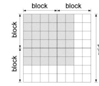
Figure 5 illustrates the sizes of grids and blocks for a reduced example. In this example, matrices H and G will have dimensions of
N × N = 6 × 6. The thread blocks were defined as containing 4 × 4 threads. From Fig. 5, it is observed that the grid will then be calculated to contain 2 × 2 blocks, in a total of 8 × 8 = 64 threads. Even so, only 6 × 6 = 36 out of the 64 threads will perform the calculations of Hij and Gij. The darkened cells in Fig. 5 represent the terms that will perform some calculation, while the blank cells represent the threads that were created, but left inactive.
Figure 5. Reduced example of a grid of thread blocks.
Two 22 × 22 sub-matrices (of H and G) are allocated at each thread block’s shared memory. The calculation of Hij and Gij performed by these threads are initially stored in these sub-matrices. In parallel execution, instead of two chain loops, each thread of the whole grid will have its own index i-j. Based on this index, the
threads will be able to univocally determine, from the data of the problem (node coordinates, element incidence, etc.) the parameters needed to perform the numerical integration of their respective Hij
and Gij. In this paper, four-node Gaussian Quadrature is adopted to perform this integration. The four terms loop referring to the Gaussian Quadrature is performed sequentially by each thread.
After all the block’s threads have ended their calculations, these data can be finally copied back to the vectors that contained H and G, allocated on the GPU’s global memory. Actually, in the present
implementation a more direct, saving-time strategy is adopted. When transferring its terms Hij and Gij from the shared memory to the global memory, each thread i-j copies them directly to the right
place of the matrices A and B, according to the boundary conditions
(see transition between Eqs. (12) and (13)). In this same step, vector
b’ (see Eq. (13)) is also assembled from u and q (see Eq. (12))
according to the boundary conditions.
In the calculation of the matrices S and D from Eq. (16), a
similar procedure is employed. The same size of thread blocks is used. The difference is that as the number of internal points might be different from the number of elements, the matrices might present more or less rows than columns, and therefore the grids will also have more or less thread blocks in their “vertical” direction.
In order to apply Eq. (16), it is also necessary that the vector x, which comes from the solution of Eq. (14), and b’ be unmixed to
form the final solution u and q at the boundary of the problem. To accomplish this switching task, one-dimensional 22 × 1 thread blocks are created. A one-dimensional grid is automatically calculated by the program to contain as many thread blocks as necessary to fit entirely the vectors u and q, which have dimensions of N × 1. This dimensioning is analogous to what was described in Fig. 5. Now, each thread of the grid has its index i and is responsible
for switching the terms xi and b’i to either ui or qi, depending on the
boundary conditions.
The remaining calculations, such as the multiplication of matrices by vectors and the solution of the linear system expressed by Eq. (14) are performed in serial execution by the CPU. There are initiatives to implement methods for solution of dense non-symmetric linear systems in GPGPU, but the present available implementations are still immature or ill-documented. Therefore, the present implementation characterizes a CPU-GPU complementary approach.
Numerical Results
The present implementation was used to solve the thermal problem depicted in Fig. 6. The problem refers to a square plate with an edge of unitary length. Each edge is discretized by N/4 equal elements. As boundary conditions, all the elements of the left border have zero temperature (u = 0), all the elements of the right
border have unit temperature (u = 1), and the remaining borders are
insulated (q = 0). This problem has a closed-form analytical solution
given by u(x) = x, according to the given system of coordinates (see
Fig. 6).
Figure 6. Two-dimensional square plate of unitary edge.
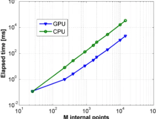
Figure 7 shows the time consumed by the CPU and the GPU to build the matrices H and G of Eq. (12) with the number of elements
N ranging from 4 to 10,000. In the GPU, this time corresponds to the time spent by the specific kernel that calculates these matrices. Notice that, in the present implementation, the threads in this kernel determine H and G and save the results of their calculations directly
into the matrices A and B according to the boundary conditions (see
Section 4 and Eqs. (12) and (13)). Therefore, the time spent on switching H and G into A and B is also included in these
measurements. In the CPU, this time corresponds to the time spent by the specific function, written in serial C code, that determines H
and G and switch their columns into A and B.
Figure 7. Time spent by the GPU and the CPU to calculate H and G and store the results directly in A and B.
At the beginning of the graphic, it can be observed that there is a number of elements under which the use of CPU is more advantageous than the GPU. The reason to that is that, in order to execute the kernel that calculates H and G on the GPU, a few allocations and copies of memory are needed, which are not necessary in the CPU. This allocation time is rather short and depends little on the number of elements N, so the increase of N causes it to dissolve in the total execution time of the kernel.
Beyond this point, the superiority of performance of the GPU is observed. In the final experiment, in which a problem of 10,000 elements was considered, the GPU obtained the matrices H and G in a time 56.8 times shorter than the CPU.
The present study also compared the time consumed to map the vectors x and b’ into the vectors u and q (see transition between Eqs.
(12) and (13)) so that the solution of up at the internal points could be determined by Eq. (16). The comparison is shown by Fig. 8.
Figure 8. Time spent by the GPU and the CPU to distribute the vectors u and q among x and b’.
It is again observed that there is a certain number of elements, upon which the use of GPU is worth. The reason is the same: there is some memory handling required before any calculation can commence. Because the calculation of the distribution of vectors and transposition of columns of matrices is much simpler than the calculation of the matrices H and G, this problem has smaller
arithmetic intensity than the prior. For this reason, the use of GPU is advantageous only from a larger number of elements (for N > 3800 elements) than in that previous investigation (for N > 10 elements).
The performance of GPU versus CPU in the calculation of internal points was also investigated. A mesh of M equally-spaced internal points was spread inside the domain of the same problem of Fig. 6. Figure 9 shows the distribution of the internal points when M = 9 internal points and N = 16 boundary elements.
Figure 9. Distribution of internal points inside the domain of the square plate.
Figure 10 reports the time spent by the GPU and the CPU to calculate the matrices S and D from Eq. (16) as the number of
internal points increase. The number of internal points (M) varies along with the number of boundary elements (N) according to the rule N = M/2. It is observed a superiority of the GPU in numerical efficiency in this calculation. In the final experiment, in which M = 14,400 internal points and N = 7,200 boundary elements were considered, the GPU obtained the matrices S and D in a time 15.16
Figure 10. Time spent by the GPU and the CPU to calculate S and D.
The calculation times reported in Fig. 10 are the ones necessary to determine the values at internal points, after the whole boundary value problem has been solved, that is, the solution of the linear system (15) and the mapping of vectors x and b’ to u and q have
been completed.
Finally, a complete problem was solved. The time spent in the solution is shown in Fig. 11 for varying number of elements N. The experiment was carried out for values of N between 4 and 6,160 elements. These times include the time to determine the influence matrices H and G, to exchange their columns into A and B and to
map the vectors u and q into x and b’ according to the boundary
conditions, and to determine the matrices S and D of internal points.
The number of internal points (M) varies along with the number of boundary elements (N) according to the rule N = M/2.
Figure 11. Times of execution to solve a complete problem.
Some parts of the GPU-CPU complementary code are executed in the CPU, such as the solution of the final system of equations (see Eq. (14)) and the matrix-vector multiplications necessary to obtain b = B⋅b’ (see Eqs. (13) and (14)) and later to
obtain up according to Eq. (16). Because these times are the same
in the GPU-CPU code as in the pure CPU code, they are not included in the results shown in Fig. 11. However, these results do include the time spent by the pair CPU-GPU with communication of data. They include the time spent to transfer the necessary data of the problem from the CPU’s RAM to the GPU’s global memory prior to the calculations, such as the vectors containing the coordinates of the nodes of the mesh and the boundary conditions. They also include the time spent to transfer back the results of the calculations from the GPU’s memory.
In previous results, some memory operations were also involved. However, those memory operations referred only to memory passing between different GPU memories, mainly the data transfer from the GPU’s global memory to the SMs’ shared memory. No memory operation between CPU and GPU was involved. Because now all the memory operations required by the complete program are taken into account, it is observed that the solution of a complete BEM problem has reduced arithmetic intensity when compared, for example, to the calculation of H and G alone. For this reason, the use of GPU is more advantageous from
a larger number of elements (for N > 27 elements) than what was observed in Fig. 7 (for N > 10 elements).
Even so, an overall superior performance of the GPU over the CPU is observed. In the final experiment, in which N = 6,160 elements and M = 12,321 internal points were considered, the graphics hardware solved the problem – both the solution at the boundary and at the internal points – in a time 15.75 times shorter than the CPU.
The RAM (global) memory of 1 GB available in the present graphics card (NVidia GeForce GTX 280) poses a limit to the number of elements that can be used. The major occupancy of memory is given by the two square matrices H and G of N × N terms, and by the two rectangular matrices D and S of M × N terms. Every term of these four matrices contains one floating-point variable of 8 bytes. Part of the memory allocated is implicitly and dynamically freed, so it is not possible to determine a priori what the limits of N and M are, but the program warns, in execution time, when the limit of memory has been reached. For the present implementation, the limits are N = 6,160 elements and M = 12,321 internal points, if the rule N = M/2 is to be followed. It is important to notice, however, that the model GeForce GTX 280 is yet thought to perform graphics calculations, for which the memory of 1 GB is enough for most situations. There are other architectures such as NVidia’s Tesla, which are specially designed for non-graphics calculations (CUDA, 2010). These special GPUs possess up to 4 GB of RAM memory. Furthermore, a different saving-memory approach could be thought for the present implementation, if a larger number of elements were necessary.
Concluding Remarks
This paper has described the implementation of the Boundary Element Method for two-dimensional potential problems on graphics processing devices. The classical serial implementation was rewritten under the SIMT parallel programming paradigm.
The paper reports the performances of GPU and CPU on dealing with three important steps of BEM: a) the calculation of the influence matrices used for the solution of the boundary values, b) the calculation of influence coefficients to determine the values at internal points, and c) the rearrangement of vectors according to the prescribed boundary conditions. It was observed that the point from which the GPU outperforms the CPU is function of the arithmetic intensity of each problem. In all the cases, however, the graphics hardware has shown to be more numerically efficient than the CPU with increasing number of elements and internal points. For the largest number of boundary elements the GPU implementations were able to outperform the CPU ones by more than one order of magnitude.
The present implementation shows that graphics cards represent a promising strategy to accelerate the numerical efficiency of the Boundary Element Method.
References
Araújo, F.C., Gray, L.J., 2008, “Evaluation of Effective Material Parameters of CNT-reinforced Composites via 3D BEM”, CMES: Computer
Beer, G., Smith, I., Duenser, C., 2009, “The Boundary Element Method with Programming: For Engineers and Scientists”, Springer.
CUDA, 2010, Developer’s Zone. http://www.nvidia.com/ object/cuda home.html.
CUDA, 2009, NVIDIA CUDA C Programming Best Practices Guide. NVIDIA Corporation, Santa Clara.
Jones, W., 2004, Beginning Directx9. Premior Press.
Kane, J.H., 1994, “Boundary Element Analysis in Engineering Continuum Mechanics”, Prentice Hall Englewood Cliffs.
Kirk, D.B., Hwu, W.M.W., 2010, “Programming Massively Parallel Processors: A Hands-On Approach”, Morgan Kaufmann Publishers.
Klöckner, A., Pinto, N., Lee, Y., Catanzaro, B., Ivanov, P., Fasih, A., 2009, “Metaprogramming Graphics Processors from High-Level Languages”, Parallel Computing (submitted).
Manavski, S.A., Valle, G., 2008, “CUDA Compatible GPU Cards as Efficient Hardware Accelerators for Smith-Waterman Sequence Alignment”, In: BMC Bioinformatics 2008, 9:1-10.
McNamee, J.M., 2004, “A comparison of methods for accurate summation”, ACM SIGSAM Bulletin, Vol. 38, No. 1.
Mesquita, E., Labaki, J., Ferreira, L.O.S., 2009, “An Implementation of the Longman’s Integration Method on Graphics Hardware”, CMES:
Computer Modeling in Engineering & Sciences, Vol. 51(2), pp. 143-168.
Nguyen, H., 2007, “GPU Gems 3”, Addison-Wesley Professional. NVidia, 2008, NVIDIA CUDA – Compute Unified Device Architecture – Programming Guide. NVIDIA Corporation, Santa Clara.
Oishi, A., Yoshimura, S., 2008, “Finite Element Analyses of Dynamic Problems Using Graphics Hardware”, CMES: Computer Modeling in
Engineering & Sciences, Vol. 25, pp. 115-131.
Owens, J.D., Luebke, D., Govindaraju, N., Harris, M., Krüger, J., Lefohn, A.E., Purcell, T.J., 2007, “A survey of general-purpose computation on graphics hardware”, Computer Graphics Forum, 26:80-113.
Peercy, M., Segal, M., Gerstmann, D., 2006, “A performance-oriented data parallel virtual machine for GPUs”, In: ACM SIGGRAPH 2006 Conference Abstracts and Applications.
Pharr, M., Fernando, R., 2005, “GPU Gems 2: Programming Techniques for High-Performance Graphics and General-Purpose Computation”, Addison-Wesley Professional.
Rasmusson, A., Mosegaard, J., Sørensen, T.S., 2008, “Exploring parallel algorithms for volumetric mass-spring-damper models in cuda”, In:
International Symposium on Computational Models for Biomedical Simulation, pp. 49-58.
Ryoo, S., Rodrigues, C.I., Baghsorkhi, S.S., Stone, S.S., Kirk, D.B., Hwu, W.M.W., 2008, “Optimization principles and application performance evaluation of a multithreaded GPU using CUDA”, In: Proceedings of the 13th ACM SIGPLAN Symposium on Principles and practice of parallel programming, February 20-23, Salt Lake City, UT, USA.
Shreiner, D., Woo, M., Neider, J., Davies, T. (eds.), 2005, “OpenGL Programming Guide”, 5th edition Addison-Wesley.
Stantchev, G., Dorland, W., Gumerov, N., 2008, “Fast parallel Particle-To-Grid interpolation for plasma PIC simulations on the GPU”, Journal of
Parallel and Distributed Computing, Vol. 68 No. 10, pp. 1339-1349.
Stantchev, G., Juba, D., Dorland, W., Varshney, A., 2009, “Using Graphics Processors for High-Performance Computation and Visualization of Plasma Turbulence”, Computing in Science and Engineering, Vol. 11, No. 2, pp. 52-59.
Takahashi, T., 2006, “GPU for BEM”, In: Proceedings of the IABEM, Symposium of the International Association for Boundary Element Methods. Editors: Schanz, M., Steinbach, O., Beer, G. and Langer, U; pp. 101-104.