Vibration attenuation and shape control of surface mounted,
embedded smart beam
Abstract
Active Vibration Control (AVC) using smart structure is used to reduce the vibration of a system by automatic modifi-cation of the system structural response. AVC is widely used, because of its wide and broad frequency response range, low additional mass, high adaptability and good efficiency. A lot of research has been done on Finite Element (FE) models for AVC based on Euler Bernoulli Beam Theory (EBT). In the present work Timoshenko Beam Theory (TBT) is used to model a smart cantilever beam with surface mounted sen-sors / actuators. A Periodic Output Feedback (POF) Con-troller has been designed and applied to control the first three modes of vibration of a flexible smart cantilever beam. The difficulties encountered in the usage of surface mounted piezoelectric patches in practical situations can be overcome by the use of embedded shear sensors / actuators. A math-ematical model of a smart cantilever beam with embedded shear sensors and actuators is developed. A POF Controller has been designed and applied to control of vibration of a flexible smart cantilever beam and effect of actuator loca-tion on the performance of the controller is investigated. The mathematical modeling and control of a Multiple In-put multiple OutIn-put (MIMO) systems with two sensors and two actuators have also been considered.
Keywords
AVC, FE, EBT, TBT, POF, MIMO, LTI, OLR, CLR
Vivek Rathi and Arshad Hussain Khan
Mechanical Engineering Department, Aligarh Muslim University, Aligarh India, 202001
Received 17 May 2012; In revised form 24 May 2012
∗ Author email: [email protected],
1 INTRODUCTION
2
Undesired noise and vibrations have always been a major problem in many human activities
3
and domains. From buildings to atomic force microscopes, all can be disturbed in their normal
4
functions by vibrations and noise. Recent technological advancements such as the availability
5
of high–power and low–cost computing, smart materials, and advanced control techniques
6
have led to a growing use of AVC systems. The implication of active control is that desirable
7
performance characteristics can be achieved through flexible and clever strategies, whereby
8
actuators excite the structure based on the structure’s response measured by sensors.
Umapathy and Bandyopadhyay[20] discussed the vibration control aspects of a smart
flex-10
ible beam for a Single Input Single Output (SISO) case. Hanagud et al. [11] developed a FE
11
model for an active beam based on EBT and applied optimal output feedback control. Hawang 12
et al.[13] developed a FE model for vibration control of a laminated plate with piezoelectric
13
sensors /and actuators. Crawley et al [9] have presented the analytical and experimental
14
development of piezoelectric actuators as elements of intelligent structures. FE models of a
15
structure containing distributed piezoelectric sensors / actuators can also be seen in [10, 24].
16
Detailed survey on various control algorithms used in active vibration control studies has been
17
presented by Alkhatib and Golnaragi [4]. A detailed comparative studies of different control
18
algorithms on active vibration control of smart beam has been presented in [14, 21]. Kumar 19
and Narayanan [15] carried out optimal location studies of sensor-actuator pairs using Linear
20
Quadratic Regulator (LQR). Li et al. [16] proposed an optimal design methodology for the
21
placement of piezoelectric actuator/sensor pairs. Molter et al. [17] carried out control design
22
analysis for flexible manipulators using piezoelectric actuators. In their paper GA technique is
23
employed for optimization of placement and size of piezoelectric material for optimal vibration
24
control. Optimal controller design for the location, size and feedback of sensor/actuators have
25
been carried out in references [12, 23].
26
Chandrashekhara andVardarajan [8] have presented a FE model of a piezoelectric
compos-27
ite beam using higher – order shear deformation theory. Aldraihem et al. [3] have developed a
28
laminated cantilever beam model using EBT and TBT with piezoelectric layers. Abramovich 29
[1] has presented analytical formulation and closed form solutions of composite beam with
30
piezoelectric actuators using TBT. Narayan and Balamurugan [18] have presented finite
el-31
ement formulation for the active vibration control study of smart beams, plates and shells
32
and the controlled response is obtained using classical and optimal control strategies. In the
33
analyses mentioned above, the controlled response has been obtained based on extension mode
34
actuation. There have been very few studies based on shear mode actuation and sensing for
35
the analysis of active structures.
36
The idea of exploiting the shear mode of creating transverse deflection in beams
(sand-37
wiched type) was first suggested by Sun and Zhang [19]. A FE approach was used by Ben-38
jeddou et al [6] to model a sandwich beam with shear and extension piezoelectric elements. It
39
was observed that the shear actuator is more efficient in rejecting vibration than the extension
40
actuator for the same control effort. Aldraihem and Khdeir [2] proposed analytical models and
41
exact solutions for beams with shear and extension piezoelectric actuators. The models are
42
based on TBT and HOBT. Exact solutions are obtained by using the state – space approach.
43
Azulay and Abramovich [5] studied the effects of actuator location and number of patches
44
on the actuator’s performance for various configurations of patches and boundary conditions
45
under mechanical and/or electrical loads.
2 POF CONTROL 47
A standard result in control theory says that the poles of a linear time invariant (LTI)
con-48
trollable system can be arbitrarily assigned by state feedback. If the original system is time
49
invariant and the linear combinations are also constrained to the time invariant, the design
50
problem is to choose an appropriate matrix of feedback gains. The problem of pole assignment
51
by piecewise constant output feedback with infrequent observation was studied by Chammas 52
and Leondes [7] for LTI systems.
53
Consider the system
54
˙
x=Ax(t)+Bu(t),
y(t)=Cx(t) (1)
Where x∈Rn, u∈Rm, y∈Rp, A∈Rn×n
, B ∈Rn×m
, C∈Rp×n 55
A, B, C are constants matrices and it is assumed that the system (A, B, C) is
control-56
lable, observable and stable. Assume that output measurements are available from system at
57
time instants t= kτ = 0, 1, 2,. . . . Now, construct a discrete LTI system from these output 58
measurements at rate 1/τ (sampling interval of τ seconds), the system so obtained is called
59
theτ system and is given by,
60
x(k+1)τ =Φτx(kτ)+Γτu(kτ)
y(kτ)=Cx(kτ) (2)
Now, design an output injection gain matrix G such that Eigen values of (Φτ +GC) are
61
inside the unit circle i.e., eig(Φτ+GC)<1. 62
u(t)=Kly(kt),
[kτ+l∆]≤t<[kτ +(l+1)∆], Kl+N =Kl
(3)
For l = 0, 1, - - - N –1, where an output sampling interval τ is divided in to
63
N subintervals of width ∆ = τ/N, the hold function being assumed constant. To see the 64
relationship between the gain sequence{Kl} and closed loop behavior, let {Φ,Γ, C} be a new
65
system and denote the system sampled at rate 1/∆ as the ∆ system and collect the gain
66
matrices Kl in to one matrix. If (Φ,Γ) system is controllable and (Φτ, C) is observable, one
67
can first choose and output injection gain G to place the eigen values of (ΦN +GC) in the 68
desired locations inside the unit circle and then compute the POF gain sequence {Kl} such
69
that,
70
ΓK=G (4)
andρ(ΦN
+GC)<1 is satisfied, where ρ is spectral radius. 71
Werner and Furuta [22] proposed the performance index so that ΓK = G need not be 72
forced exactly. This constraint is replaced by a penalty function, which makes it possible to
73
enhance the closed loop performance by allowing slight deviations from the original design and
74
at the same time improving behavior. The performance index is,
J(k)= ∞
∑
l=0
[ xTl uTl ] [ Q 0
0 R ] [ xl
ul ]+
∞
∑
k=1
(xkN−x∗kN) T
P(xkN−x∗kN) (5)
Where,R∈Rm×n
, Q and P ∈Rn×n
,are positive definite and symmetric weight matrices.
76
The first term represents ’averaged’ state and control energy whereas the second term penalizes
77
deviation of G.
78
3 FORMULATION
79
3.1 Surface Mounted Sensors and Actuators 80
The smart cantilever model is developed using a piezoelectric beam element, which includes
81
sensor and actuator dynamics and a regular beam element based on TBT assumptions. The
82
piezoelectric beam element is used to model the regions where the piezoelectric patch is bonded
83
as sensor/actuator, and rest of the structure is modeled by the regular beam element.
84
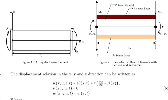
The longitudinal axis of the regular beam element (Fig. 1), lies along the X – axis. The
85
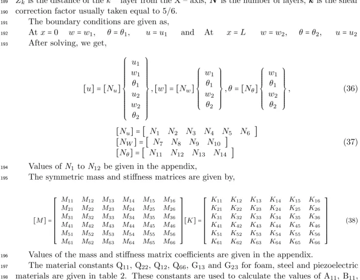
element has constant moment of inertia, modulus of elasticity, mass density and length. The
86
element is assumed to have two degree of freedom, a transverse shear force and a bending
87
moment act at each nodal point.
88
θ
θ
Figure 1 A Regular Beam Element
θ θ
Figure 2 Piezoelectric Beam Elements with Sensors and Actuators
The displacement relation in the x, y and z direction can be written as,
89
u(x, y, z, t)=zθ(x, t)=z(∂w
∂x −β(x)),
v(x, y, z, t)=0, w(x, y, z, t)=w(x, t)
(6)
Where,
90
w is the time dependent transverse displacement of the centroidal axis, θ is the time
91
dependent rotation of the cross – section about ‘Y – axis’.
For the static case with no external force acting on the beam, the equation of motion is,
93
∂[κGA(∂w∂x +θ)]
∂x =0,
∂(EI∂x∂θ)
∂x −κGA( ∂w
∂x +θ)=0 (7)
The boundary conditions are given as,
94
At x=0 w=w1, θ=−θ1 and At x=L w=w2, θ=−θ2
95
The mass matrix is given by,
96
[M]=
L
∫ 0
[ [Nw] [Nθ] ]
T
[ ρA0 ρI0
yy ] [ [
Nw] [Nθ] ]
dx (8)
[M]=[MρA]+[MρI] (9)
[MρA] in equation is associated with translational inertia and [MρI] is associated with
97
rotary inertia, there expressions are given in the appendix.
98
The stiffness matrix is given by,
99
[K]=
L
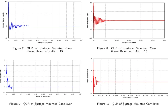
∫ 0
[ ∂x∂ [Nθ] [Nθ]+∂x∂ [Nw] ]
T
[ EI0 κGA0 ]×[
∂ ∂x[Nθ] [Nθ]+∂x∂ [Nw] ]
dx (10)
Finally we obtain;
100
[K]= EI
(1+ϕ)L3
⎡⎢ ⎢⎢ ⎢⎢ ⎢⎢ ⎣
12 6L −12 6L
6L (4+ϕ)L2 −6L (2−ϕ)L2 −12 −6L 12 −6L
6L (2−ϕ)L2 −6L (4+ϕ)L2
⎤⎥ ⎥⎥ ⎥⎥ ⎥⎥ ⎦
(11)
Hereϕis the ratio of the beam bending stiffness to the shear stiffness given by,ϕ= 12
L2( EI κGA),
101
Lis the length of beam element. E is the Young’s modulus of the beam material,Gis shear
102
modulus of the beam material, k is shear coefficient which depends on the material definition
103
and cross – sectional geometry, I is the moment of inertia of the beam element, A is the area
104
of cross – section of the beam element and ρ is the mass density of the beam material.
105
The consistent force array is given as,
106
{F}=
L
∫ 0
[ [Nw] [Nθ] ]
T
{ mq }dx. (12)
The piezoelectric element is obtained by sandwiching the regular beam element between two
107
thin piezoelectric layers as shown in figure 2. The element is assumed to have two – structural
108
degree of freedom at each nodal point and an electric degree of freedom. The piezoelectric
layers are modeled based on EBT as the effect of shear is negligible and the middle steel layer
110
is modeled based on TBT. The mass and stiffness matrix of piezoelectric layers is given by,
111
[Mp]= ρpAplp
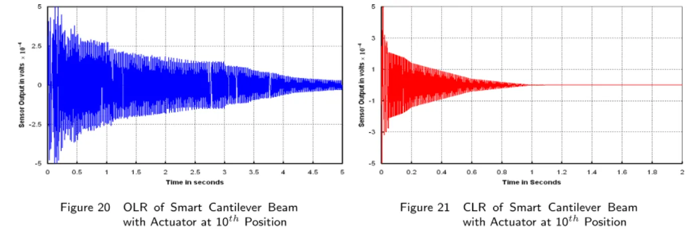
420 ⎡⎢ ⎢⎢ ⎢⎢ ⎢⎢ ⎣
156 22lp 54 −13lp
22lp 4l
2
p 13lp −3l
2
p
54 13lp 156 −22lp
−13lp −3lp2 −22lp 4l2p ⎤⎥ ⎥⎥ ⎥⎥ ⎥⎥ ⎦
[Kp]= EpIp lp ⎡⎢ ⎢⎢ ⎢⎢ ⎢⎢ ⎢⎢ ⎣ 12 l2 p 6
lp − 12 l2 p 6 lp 6
lp 4 −
6
lp 2 −12l2
p − 6 lp 12 l2 p − 6 lp 6
lp 2 −
6
lp 4
⎤⎥ ⎥⎥ ⎥⎥ ⎥⎥ ⎥⎥ ⎦ (13)
ρp is the mass density of piezoelectric beam element, Ap is the area of piezoelectric patch
112
= 2 tac, lp (=L) is the length of the piezoelectric patch. Ep is the modulus elasticity of
113
piezoelectric material, Ip is the moment of inertia of piezoelectric layer w. r. t. the neutral
114
axis of the beam
115
Ip=
1 12ct
3
a+cta[(
ta+tb)
2 ]
2
ta is the thickness of actuator,tb is the thickness of beam,c is the width of beam.
116
The mass matrix for the piezoelectric beam element is given by,
117
[Mpiezo]=[MρA]+[MρI]+[Mp] (14)
Stiffness matrix [Kpiezo]for the piezoelectric beam element,
118
[Kpiezo]=[K]+[Kp] (15)
3.1.1 Piezoelectric Strain Rate Sensors and Actuators 119
The linear piezoelectric coupling between the elastic field and the electric field can be expressed
120
by the direct and converse piezoelectric equations, respectively,
121
D=dσ+eTEf ε=sEσ+dEf (16)
σ is the stress, ϵis the strain, Ef is the electric field, e is the permittivity of the medium,
122
SE is the compliance of the medium, d is the piezoelectric constants.
123
Sensor Equation: If the poling is done along the thickness direction of the sensors with
124
the electrodes on the upper and lower surfaces, the electric displacement is given by,
125
Dz =d31×Epεx=e31εx (17)
e31is the piezoelectric stress / charge constants,Epis the Young’s modulus of piezoelectric
126
material, ϵx is the strain of the testing structure at a point.
127
The sensor output voltage is,
128
Vs(t)=Gce31zc
lp
∫ 0
nT
l is the second spatial derivative of the shape function of the flexible beam and as a scalar
129
vector product as,
130
Vs(t)=pT˙q (19)
˙q is the time derivative of the displacement vector, pT is a constant vector.
131
The input voltage to an actuator is Va(t) given by,
132
Va(t)=KVs(t) (20)
Actuator Equation: The strain developed by the electric field(Ef)on the actuator layer
133
is given by,
134
εA=d31Ef (21)
The control force applied by the actuator is,
135
fctrl=Epd31cz ∫ lp
n2.dx.Va(t). (22)
z= (ta+tb)
2 , is the distance between the neutral axis of the beam and the piezoelectric layer.
136
Or as a scalar product as,
137
fctrl=h.Va(t) (23)
nT
2 is the first spatial derivative of shape function of the flexible beam, hT is a constant
138
vector.
139
If any external forces described by the vector fext are acting then, the total force vector
140
becomes,
141
ft=fext+fctrl (24)
3.1.2 Dynamic Equation and State Space Model 142
The dynamic equation of motion of the smart structure is finally given by,
143
M.¨q +K.q=fext+fctrl (25)
q=T.g , (26)
T is the model matrix containing the eigen vectors representing the desired number of
144
modes of vibration of the cantilever beam, g is the modal coordinate vector.
145
Equation (25) is then transformed in to,
146
M∗
M∗
is the generalized mass matrixK∗
is the generalized stiffness matrix, C∗
is the
gener-147
alized damping matrix, f∗
ext is the generalized external force vectors, f∗ctrl is the generalized
148
control force vectors. The structural modal damping matrix is-:
149
C∗
=αM∗+βK∗, (28)
α andβ are constants.
150
The state space model is
151 ⎡⎢ ⎢⎢ ⎢⎢ ⎢⎢ ⎣ ˙ x1 ˙ x2 ˙ x3 ˙ x4 ⎤⎥ ⎥⎥ ⎥⎥ ⎥⎥ ⎦
=[ 0 I
−M∗−1K∗ −M∗−1C∗ ]
⎡⎢ ⎢⎢ ⎢⎢ ⎢⎢ ⎣ x1 x2 x3 x4 ⎤⎥ ⎥⎥ ⎥⎥ ⎥⎥ ⎦
+[ M∗−01
TTh ] u(t)+[
0 M∗−1
TTf ] r(t) (29)
u (t) is the control input,r (t) is the external input to the system,f is the external force
152
coefficient vector. The sensor equation for the modal state space form is given by;
153
y(t)=[ 0 pT T ]
⎡⎢ ⎢⎢ ⎢⎢ ⎢⎢ ⎣ x1 x2 x3 x4 ⎤⎥ ⎥⎥ ⎥⎥ ⎥⎥ ⎦ (30)
The above system may be represented as,
154
˙x=A.x(t)+B.u(t)+E. r(t) (31)
y(t)=CTx(t) (32)
3.1.3 Validation for Surface Mounted Smart Beam 155
To validate the present formulation and the computer program, a cantilever beam made of steel
156
which is surface bonded with two PZT layers on both side is considered. The elastic modulus,
157
poisons ratio and density of steel and PZT are 200GPa, 0.3 and 7500 Kg/m3
and 139 GPa,
158
0.3 and 7500 Kg/m3
respectively while the strain and stress constants of PZT are 23×10−12
159
m/V and 0.216 respectively [8]. The length, width and the thickness of the beam are 500 mm,
160
30 mm and 2 mm respectively while the thickness of each of the PZT layers is 40 µm. The
161
Voltages at the steel and PZT layers are set to zero. The beam is discretized into 20 elements to
162
obtain converged results. The beam is excited with 0.2×10⁻³Ns impulse load acting on the tip 163
of the beam. The closed loop response of the tip displacement is obtained using constant gain
164
negative velocity feedback (CGVF) control with gain Gv =1 and linear quadratic Regulator
165
(LQR) control Q=106
and R=1 and compared with the response obtained under the same
166
condition by the Narayanan and Balamurugan [8]. The control is applied after 0.5 seconds.
167
The present response of the system is very well matched with the published results. Next, the
first six open-loop and closed-loop natural frequencies of beam are presented in Table 1 and
169
compared with reference [18]. These frequencies are in good agreement with the published
170
results.
171
Table 1 First six natural frequencies of smart steel cantilever beam
Open loop natural Closed loop natural Closed loop natural Natural frequencies (Hz) frequencies (Hz) frequencies (HZ) frequencies (Hz) (CGVF control) (LQR control) [8]
6.809 6.855 6.834 6.89 41.64 43.19 41.69 43.285 115.7 121.6 115.7 121.225 226.2 237.5 226.3 237.72 373.6 357.5 373.7 393.58 557.8 506.3 557.9 589.63
Figure 3 Closed loop response of smart cantilever steel beam (a)Narayanan and Balamurugan[18](reproduced with permission from Elsevier) and (b) Present obtained with negative CGVF control withGv=1.
Figure 4 Closed loop response of smart cantilever steel beam (a)Narayanan and Balamurugan[18] (reproduced with permission from Elsevier) and (b) Present obtained with LQR control withQ=106andR=1.
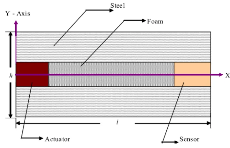
3.2 Embedded Shear Sensors And Actuators 172
The piezoelectric element is embedded on discrete locations of the sandwich beam as shown in
173
Figure (5). The smart cantilever beam model is developed using a piezoelectric sandwich beam
174
element, which includes sensor and actuator and a regular sandwiched beam element, which
175
includes foam at the core. A FE model of a piezoelectric sandwich beam is developed using
laminate beam theory. It consists of three layers. The assumption made is that the middle
177
layer is perfectly glued to the carrying structure and the thickness of adhesive can be neglected
178
and each layer behaves as a Timoshenko beam. The longitudinal axis of the sandwiched beam
179
element lies along the X – axis. The element has constant moment of inertia, modulus of
180
elasticity, mass density and length. The element is assumed to have three degree of freedom,
181
a transverse shear force and a bending moment act at each nodal point.
182
Figure 5 A Sandwiched Beam Element
The displacement relation of the beam u (x, z) and wu (x, z) can be written as,
183
u(x, z)=u0(x)−zθ(x, t) w(x, z)=w0(x) (33)
u0(x)andw0(x) are the axial displacements of the point at the mid plane,θ(x) is the
184
bending rotation of the normal to the mid plane.
185
The beam constitutive equation can be written as,
186
⎡⎢ ⎢⎢ ⎢⎢ ⎣
Nx
Mx
Qxz ⎤⎥ ⎥⎥ ⎥⎥ ⎦
=
⎡⎢ ⎢⎢ ⎢⎢ ⎣
A11 B11 0
B11 D11 0
0 0 A55
⎤⎥ ⎥⎥ ⎥⎥ ⎦ ⎡⎢ ⎢⎢ ⎢⎢ ⎣
∂u0 dx ∂θ ∂x
θ+∂w0 ∂x
⎤⎥ ⎥⎥ ⎥⎥ ⎦
+
⎡⎢ ⎢⎢ ⎢⎢ ⎣
E11
F11
G55
⎤⎥ ⎥⎥ ⎥⎥ ⎦
(34)
A11,B11,D11 and A55 are the extensional, bending and shear stiffness coefficients defined
187
according to the lamination theory,
188
A11=c
N
∑
k=1
(Q11)k(zk−zk−1),
B11=c
N
∑
k=1
(Q11)k(z 2
k−z
2
k−1),
D11= c3
N
∑
k=1
(Q11)k(z 3
k−z
3
k−1)
(35)
A55=cκ
N
∑
k=1
Zk is the distance of thekth layer from the X – axis,N is the number of layers, k is the shear
189
correction factor usually taken equal to 5/6.
190
The boundary conditions are given as,
191
At x=0 w=w1, θ=θ1, u=u1 and At x=L w=w2, θ=θ2, u=u2
192
After solving, we get,
193
[u]=[Nu]
⎧⎪⎪⎪⎪ ⎪⎪⎪⎪⎪ ⎪⎪ ⎨⎪⎪⎪ ⎪⎪⎪⎪⎪ ⎪⎪⎪⎩ u1 w1 θ1 u2 w2 θ2 ⎫⎪⎪⎪⎪ ⎪⎪⎪⎪⎪ ⎪⎪ ⎬⎪⎪⎪ ⎪⎪⎪⎪⎪ ⎪⎪⎪⎭
,[w]=[Nw]
⎧⎪⎪⎪⎪ ⎪⎪ ⎨⎪⎪⎪ ⎪⎪⎪⎩ w1 θ1 w2 θ2 ⎫⎪⎪⎪⎪ ⎪⎪ ⎬⎪⎪⎪ ⎪⎪⎪⎭
, θ=[Nθ]
⎧⎪⎪⎪⎪ ⎪⎪ ⎨⎪⎪⎪ ⎪⎪⎪⎩ w1 θ1 w2 θ2 ⎫⎪⎪⎪⎪ ⎪⎪ ⎬⎪⎪⎪ ⎪⎪⎪⎭ , (36)
[Nu]=[ N1 N2 N3 N4 N5 N6 ]
[NW]=[ N7 N8 N9 N10 ]
[Nθ]=[ N11 N12 N13 N14 ]
(37)
Values of N1toN12 be given in the appendix,
194
The symmetric mass and stiffness matrices are given by,
195
[M]= ⎡ ⎢ ⎢ ⎢ ⎢ ⎢ ⎢ ⎢ ⎢ ⎢ ⎢ ⎢ ⎣
M11 M12 M13 M14 M15 M16
M21 M22 M23 M24 M25 M26
M31 M32 M33 M34 M35 M36
M41 M42 M43 M44 M45 M46
M51 M52 M53 M54 M55 M56
M61 M62 M63 M64 M65 M66
⎤ ⎥ ⎥ ⎥ ⎥ ⎥ ⎥ ⎥ ⎥ ⎥ ⎥ ⎥ ⎦
[K]= ⎡ ⎢ ⎢ ⎢ ⎢ ⎢ ⎢ ⎢ ⎢ ⎢ ⎢ ⎢ ⎣
K11 K12 K13 K14 K15 K16
K21 K22 K23 K24 K25 K26
K31 K32 K33 K34 K35 K36
K41 K42 K43 K44 K45 K46
K51 K52 K53 K54 K55 K56
K61 K62 K63 K64 K65 K66
⎤ ⎥ ⎥ ⎥ ⎥ ⎥ ⎥ ⎥ ⎥ ⎥ ⎥ ⎥ ⎦ (38)
Values of the mass and stiffness matrix coefficients are given in the appendix.
196
The material constants Q11, Q22, Q12, Q66, G13 and G23 for foam, steel and piezoelectric
197
materials are given in table 2. These constants are used to calculate the values of A11, B11,
198
D11 and A55
199
Table 2 Material Properties and Constants
Material Constants Piezoelectric Material Steel Foam
G12(MPa) 24800 78700 99.9
G13(MPa) 24800 78700 99.9
G23(MPa) 24800 78700 99.9
d31(m/V) -16.6×10 −9
# #
d15(m/V) 1.34×10 −9
# #
Q11(MPa) 68400 215000 85.4
Q22(MPa) 68400 215000 85.4
Q12(MPa) 12600 2880 75.8
Q66(MPa) 12600 78700 9.99
Sensor Equation: The charge q(t) accumulated on the piezoelectric electrodes is given
200
by,
q(t)=∬
A
D3dA (39)
D3is the electric displacement in the thickness direction, A is the area of electrodes.
202
The current induced in sensor layer is converted in to the open circuit sensor voltage
203
Vs(t) using a signal-conditioning device with a gain of Gc and applied to the actuator with
204
the controller gain Kc.
205
Vs(t)=Gci(t), Vs(t)=e15c 6η
(−12η+l2)[ 0 2 −l 0 −2 −l ] [q˙], V
s(t)=[p]T[
˙
q] 206
[q˙] is the time derivative of the modal coordinate vector,[p]T is a constant vector.
207
The input voltage of the actuator is Va(t), given by,
208
Va(t)=KcVs(t) (40)
Actuator Equation: The strain produced in the piezoelectric layer is directly
propor-209
tional to the electric potential applied to the layer.
210
γxz∝Ef
γxz is the shear strain in the piezoelectric layer, Ef is the electric potential applied to the
211
actuator.
212
From the constitutive piezoelectric equation, we get,
213
γxz=d15Ef (41)
The shear force Qxz is given as
214
Qxz=cGd15
Va (t)
tp
tp
∫ 0
dz (42)
Or as a scalar product,
215
fctrl=h. Va (t) (43)
Where,fctrl=Qxzand hT is a constant vector.
216
If any external forces described by the vector fctrl are acting, then total force vector
be-217
comes,
218
3.2.1 Dynamic Equation and State Space Model: 219
The dynamic equation is,
220
M∗
.¨g+C∗.˙g+K∗.g=fext∗ +fctrl∗ (45)
C∗
= αM∗+βK∗, (46)
The state space form of the system is obtained as,
221 ⎡⎢ ⎢⎢ ⎢⎢ ⎢⎢ ⎢⎢ ⎢⎢ ⎢⎣ ˙ x1 ˙ x2 ˙ x3 ˙ x4 ˙ x5 ˙ x6 ⎤⎥ ⎥⎥ ⎥⎥ ⎥⎥ ⎥⎥ ⎥⎥ ⎥⎦
=[ 0 I
−M∗−1K∗ −M∗−1C∗ ]
⎡⎢ ⎢⎢ ⎢⎢ ⎢⎢ ⎢⎢ ⎢⎢ ⎢⎣ x1 x2 x3 x4 x5 x6 ⎤⎥ ⎥⎥ ⎥⎥ ⎥⎥ ⎥⎥ ⎥⎥ ⎥⎦
+[ M∗−01
TTh ]u(t)+[
0
M∗−1
TTf ]r(t) (47)
The sensor equation for the modal state space form is given by;
222
y(t)=[ 0 pT T ]
⎡⎢ ⎢⎢ ⎢⎢ ⎢⎢ ⎢⎢ ⎢⎢ ⎢⎣ x1 x2 x3 x4 x5 x6 ⎤⎥ ⎥⎥ ⎥⎥ ⎥⎥ ⎥⎥ ⎥⎥ ⎥⎦ (48)
The above system can be represented as,
223
˙x=A.x(t)+B.u(t)+E. r(t) (49)
y(t)=CTx(t) (50)
4 SIMULATION
224
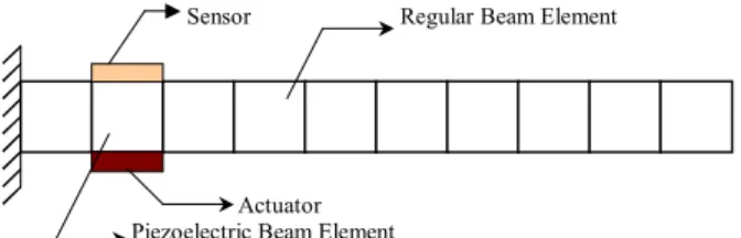
4.1 Simulation of Surface Mounted Sensors and Actuators 225
The state space representation of the cantilever beam with the surface mounted sensor /
226
actuator is obtained by using nine regular beam elements and one piezoelectric element as
227
shown figure (6).
228
The dimensions and properties of the flexible beam and piezoelectric sensor / actuator used
229
in the numerical simulation are given in tables 3 and 4 respectively.
230
Two state space models of the smart cantilever beam have been obtained by keeping the
231
AR 8 and 15, the length of the beam is kept constant and the thickness of the beam is varied.
Figure 6 Cantilever Beam with Surface Mounted Sensors and Actuators Table 3 Physical Properties of Steel Beam
Total length of beam (mm) l 500 Width (mm) b 24 Young’s modulus (Pa) Eb 193x109
DensityKg/m3
) ρb 8030
Constants used in C∗
α, β 10−3 ,10−4
The POF control technique is used to design a controller to suppress vibration of a cantilever
233
beam. For this purpose three vibration modes are considered. In the first case the AR is
234
taken equal to 15. Configuration specifications of smart beam are as per table 3 and 4. The
235
collocated sensor and actuator are placed near the fixed end. The FE model of the surface
236
mounted cantilever beam is developed in MATLAB using TBT. A sixth order space model
237
of the system is obtained on retaining the first three modes of vibration of the system. The
238
first three natural frequencies calculated are 106.03 Hz,658.33Hz, 1826.38Hz respectively. An
239
impulsive force of 10N is applied for duration of 0.05sec and the open loop response (OLR) of
240
the system is obtained as shown in figure 7. A controller based on the POF control algorithm
241
has been designed to control the first three modes of vibration of the smart cantilever beam.
242
The sampling interval used is 0.0004 sec. The sampling interval is divided in to 10 subintervals
243
(N=10). The periodic output gain for the system is obtained by using the algorithm given for
244
POF controller, the impulse response of the system with POF gain is shown in figure 8.
245
In the second case the AR is taken equal to 8, and again all other parameters are kept
246
same as that in the first case for which AR is 15. The first three natural frequencies calculated
247
are 197.94Hz, 1215.89Hz and 3311.05Hz respectively. The OLR and CLR (with POF gain) of
248
the system is obtained as shown in figure 9 and 10.
249
Table 4 Properties of Piezoelectric Sensor /Actuator Width (mm) b 24 Thickness (mm) ta 0.5
Young’s Modulus (Pa) Ep 68x109
Density(Kg/m3
) ρp 7700
Piezoelectric strain Constant (mV−1
) d31 125x10-12
Piezoelectric stress Constant (VmN−1
Figure 7 OLR of Surface Mounted
Can-tilever Beam with AR = 15 Figure 8 CLR of Surface Mounted Can-tilever Beam with AR = 15
Figure 9 OLR of Surface Mounted Cantilever
Beam with AR = 8 Figure 10 CLR of Surface Mounted CantileverBeam with AR = 8
The variation of control signal with time is shown in figure 11 (for AR = 15) and 12(for
250
AR = 8).
251
A POF controller is designed for the Timoshenko beam models. Two cases (AR=15,8)
252
have been considered. By comparing the OLR and CLR in the first case for AR=15, we
253
observed that there was a 89.43% decrease in settling time for the system after applying POF
254
control, and a change of 89% in settling time was observed for the case with AR=8. Thus, it
255
can be inferred from the simulation results, that a POF controller applied to a smart cantilever
256
model based on TBT is able to satisfactorily control higher modes of vibration of the smart
257
cantilever beam for a wide range of AR.
Figure 11 Control Signal of Surface Mounted
Cantilever Beam with AR = 15 Figure 12 CLR of Surface Mounted CantileverBeam with AR = 8
4.2 Simulation of Embedded Sensors and Actuators 259
4.2.1 Single Input Single Output (SISO) System 260
The FE model of smart cantilever beam based on laminate beam theory is developed. Keeping
261
the sensor location fixed and varying the position of the actuator, different state space models
262
of the smart cantilever beam are obtained. A POF controller is designed to control the first
263
three modes of vibration of the smart cantilever beam. Here an attempt has been made to find
264
the optimum actuator position for a single input single output (SISO) system. Three cases
265
have been considered.
266
In the first case FE model of the smart cantilever beam is obtained by dividing the beam
267
into 10 elements. The actuator is placed as the 1st element (at the fixed end) and the sensor
268
is placed as the 8thelement as shown in figure 13. The length of beam is 200mmand its cross
269
– section is 10mm×20mm. The length of piezoelectric patch is 200mmand its cross – section
270
is 6mm×20mm. The material properties used for the generation of FE model are given in
271
table 2. A ninth order space model of the system is obtained on retaining the first three modes
272
of vibration of the system. The first three natural frequencies (same for all three models) are
273
44.9 Hz, 82.4 Hz and 131.5 Hz respectively.
274
Figure 13 Smart Cantilever Beam with Actuator at 1stPosition and Sensor at 8thPosition
An impulsive force of 10N is applied for duration of 0.05sec and the OLR of the system
275
is obtained as shown in figure 14 A controller based on the POF control algorithm has been
276
designed to control the first three modes of vibration of the smart cantilever beam. The
277
sampling interval used is 0.07 m sec. The sampling interval is divided in to 10 subintervals (N
278
=10). The impulse response or CLR of the system with POF gain is shown in figure 15.
Figure 14 OLR of Smart Cantilever Beam with Actuator at1stPosition
Figure 15 CLR of Smart Cantilever Beam with Actuator at1stPosition
In the second case, the actuator is placed as the 5th element and the sensor is placed as
280
the 8thelement as shown in figure 17. Other parameters are kept same.
281
Figure 16 Smart Cantilever Beam with Actuator at 5thPosition and Sensor at 8thPosition
An impulsive force of 10 N is applied for duration of 0.05sec and the OLR of the system is
282
obtained as shown in figure 17. The CLR of the system with POF gain is shown in figure 18.
283
Figure 17 OLR of Smart Cantilever Beam with Actuator at5thPosition
Figure 18 CLR of Smart Cantilever Beam with Actuator at5thPosition
In the third case, the actuator is placed as the 10thelement (at the free end) and the sensor
284
is placed as the 8th element as shown in figure 19. Other parameters are kept same as that of
285
first case.
286
An impulsive force of 10 N is applied for duration of 0.05sec and the OLR of the system is
Figure 19 Smart Cantilever Beam with Actuator at 1stPosition and Sensor at 8thPosition
obtained as shown in figure 20. The impulse response of the system with POF gain is shown
288
in figure 21.
289
Figure 20 OLR of Smart Cantilever Beam with Actuator at 10thPosition
Figure 21 CLR of Smart Cantilever Beam with Actuator at 10thPosition
The variation of control signal with time for all the three cases are shown in figure 22 to
290
24.
291
Figure 22 Control Signal of Smart Cantilever Beam with Actuator Placed at 1st
Position
Figure 23 Control Signal of Smart Cantilever Beam with Actuator at 5thPosition
Here in the present case, the performance of the controller is evaluated for different actuator
292
locations while the position of the sensor is kept constant. It can be inferred from the response
293
characteristics that the actuator locations has negligible effect on the performance of the
294
controller.
Figure 24 Control Signal of Smart Cantilever Beam with Actuator at 10thPosition
4.2.2 Multi – Input Multi – Output (MIMO) Systems
296
Active control of vibration of a smart cantilever beam through smart structure concept for a
297
multivariable system (MIMO) case is considered here. The structure is modeled in space state
298
from using Finite element method by dividing the beam in to 10 FE and placing the sensors
299
at the 6thand 10thpositions and the actuators at the 4th and 8th position. Thus giving rise
300
to MIMO with two actuator inputs u1 and u2 and two sensors outputs y1and y2, The POF
301
control technique is used to design a controller to suppress the first three modes of vibration
302
of a smart cantilever beam for a multi variable system. The simulations are carried out in
303
MATLAB. The parameters are kept same as that of the model used for SISO case. The first
304
three natural frequencies calculated are 45.2 Hz, 83.2 Hz and 136.4 Hz respectively.
305
Figure 25 A MIMO Smart Cantilever Beam with Two Inputs and Two Outputs
An impulsive force of 10N is applied for duration of 0.05sec. A controller based on the
306
POF control algorithm has been designed to control the first three modes vibration of the
307
smart cantilever beam for the multivariable case. The CLR (sensor outputs y1and y2) with
308
periodic output feedback gain K for the state space model of the system is shown in figure 27
309
and 31. Figures 29 and 33 show the variation of the control signal with time.
Figure 26 CLR of SISO System with Sensor
at 6thPosition Figure 27 Response y
1 of MIMO System
with POF
Figure 28 Control Input of SISO System with Sensor at 6th Position and
Actuator at 4thPosition
Figure 29 Control Inputu1 of MIMO
Sys-tem with POF
It can be inferred from the simulation results, that the system’s performance meets the
311
design requirements. It is also observed that the maximum amplitude of the sensor output
312
voltage is less for the multivariable case and the response takes lesser time to settle. Controlling
313
time is considerably reduced with MIMO systems as compared to SISO systems.
Figure 30 30 CLR of SISO System with Sen-sor at 10thPosition and Actuator
at 8thPosition
Figure 31 Response y2 of MIMO System
with POF
Figure 32 Control Input of SISO System with Sensor at 10thPosition and
Actuator at 8thPosition
Figure 33 Control Input u2 of MIMO
Sys-tem with POF
5 CONCLUSION: 315
An integrated FE model to analyze the vibration suppression capability of a smart cantilever
316
beam with surface mounted piezoelectric devices based on TBT is developed. In practical
317
situations a large number of modes of vibrations contribute to the structures response. In this
318
work a FE model of a smart cantilever beam have been obtained by varying the AR from
319
8 to 15, the length of the beam is kept constants and the thickness of the beam is varied.
320
POF control technique is used to design a controller to suppress the vibration of the smart
321
cantilever beam by considering three modes of vibration. Two different cases have been
con-322
sidered (AR=8,15). The simulation results show that the POF controller based on TBT is
323
able to satisfactorily control the first three modes of vibration of the smart cantilever beam
324
for different AR. Surface mounted piezoelectric sensors and actuators are usually placed at
325
the extreme thickness positions of the structure to achieve most effective sensing and
actua-326
tion. This subjects the sensors / actuators to high longitudinal stresses that might damage
327
the piezoceramic material. Furthermore, surface mounted sensors/ actuators are likely to be
328
damaged by contact with surrounding objects. Embedded shear sensors / actuators can be
329
used to alleviate these problems. A FE model of a smart cantilever beam with embedded
piezoelectric shear sensors / actuators based on laminate theory is developed.
331
A POF controller is designed to control the vibration of the system. The performance of
332
the controller is evaluated for different actuator locations while the position of sensor is kept
333
constant. It was observed from the simulation results that the location of the actuator has
334
negligible effect on the performance of the controller. A MIMO system with two sensors and
335
two actuators has also been considered. A POF controller has been designed for the MIMO
336
smart structure model to control the vibration of the system by considering the three modes
337
of vibration. The beam with embedded shear sensors / actuators has been divided in to 10 FE
338
with the sensors placed at the 6th and 10th positions and the actuators placed at the 4th and
339
8th positions. It can be inferred from the simulation results, that when the system is placed
340
with the controller, the system’s performance meets the design requirements. It is observed
341
that the maximum amplitude of the sensor output voltage is less for the multivariable case
342
and the response takes lesser time to settle.
343
APPENDIX 344
1. Translational mass matrix:
345
[MρA]=
ρI 210(1+φ)2
⎡⎢ ⎢⎢ ⎢⎢ ⎢⎢ ⎢⎢ ⎣
[70φ2
+147φ+78] [35φ2
+77φ+44]L4 [35φ 2
+63φ+27] −[35φ2
+63φ+26]L4
[35φ2
+77φ+44]L4 [7φ 2
+14φ+8]L 2
4 [35φ 2
+63φ+26]L4 −[7φ 2
+14φ+6]L 2
4
[35φ2
+63φ+27] [35φ2+63φ+26]L4 [70φ 2
+147φ+78] −[35φ2+77φ+44]L4
−[35φ2
+63φ+26]L4 −[7φ 2
+14φ+6]L 2
4 −[35φ 2
+77φ+44]L4 [7φ 2
+14φ+8]L 2 4 ⎤⎥ ⎥⎥ ⎥⎥ ⎥⎥ ⎥⎥ ⎦ 346
2. Rotational Mass matrix
347
[MρI]= ⎡⎢ ⎢⎢ ⎢⎢ ⎢⎢ ⎣
36 −(15ϕ−3)L −36 −(15ϕ−3)L
−(15ϕ−3)L (10ϕ2+5ϕ+4)L2 (15ϕ−3)L (5ϕ2−5ϕ−1)L2
(10ϕ2
+5ϕ+4)L2 (15ϕ−3)L 36 (15ϕ−3)L −(15ϕ−3)L (5ϕ2−5ϕ−1)L2 (15ϕ−3)L (10ϕ2+5ϕ+4)L2
⎤⎥ ⎥⎥ ⎥⎥ ⎥⎥ ⎦
3. The mass matrix for the sandwich beam element ,
348
[M]=
⎡⎢ ⎢⎢ ⎢⎢ ⎢⎢ ⎢⎢ ⎢⎢ ⎢⎣
M11 M12 M13 M14 M15 M16
M21 M22 M23 M24 M25 M26
M31 M32 M33 M34 M35 M36
M41 M42 M43 M44 M45 M46
M51 M52 M53 M54 M55 M56
M61 M62 M63 M64 M65 M66
⎤⎥ ⎥⎥ ⎥⎥ ⎥⎥ ⎥⎥ ⎥⎥ ⎥⎦ Where, 349
M11= 1
3LI1, M12=M21= 1 2
γ L2
I1
(12η−L2), M13=M31=− 1 4
γ L3
I1
350
M15=M51=− 1 2
γ L2I1
(12η−L2), M16=M61=−
1 4
γ L3I1
(12η−L2), M24=M42=
1 2
γ L2I1
(12η−L2),
M22= 1 35
L⎛⎜
⎝
−294I3ηL 2
+35I2L 3
+1680I2η 2
+13I3L 4
−420I2ηL
+42I1L 2
+42γ2I1L 2
⎞ ⎟ ⎠
(12η−L2)2 ,
M23=M32= 1 210
L⎛⎜
⎝ 11I3L
5
−10080I2η 2
+1260I3η 2
L−231I3L 3
η+126γ2I1L 3
+1260LI1η+840I2ηL 2
+21I1L 3
⎞ ⎟ ⎠
(12η−L2)2 ,
M25=M52= 3 70
L(3I3L4−28γ2I
1L2−28I1L2−84I3ηL2+560I3η2)
(12η−L2)2 ,
M26=M62= 1 420
L⎛⎜
⎝
13I3L5+10080I2η2+2520I3η2L−378I3L3η+252γ2I1L3
−2520LI1η−840I2ηL2−42I1L3
⎞ ⎟ ⎠ (12η−L2)2
351
M55= 1 35
L⎛⎜
⎝
13I3L4−35I2L3+42γ2I1L2+42I1L2−294I3ηL2
+420I2ηL+1680I3η 2
⎞ ⎟ ⎠
(12η−L2)2 ,
M56=M65= 1 210
L⎛⎜
⎝
11I3L5+10080I2η2+1260I3η2L−231I3L3η+126γ2I1L3
+1260LI1η−840I2ηL2+21I1L3
⎞ ⎟ ⎠
(12η−L2)2 ,
M66= 1 210
L⎛⎜
⎝
252I3η 2
L2
−42I3L 4
η+10080I1η 2
+63γ2I1L 4
+28I1L 4
−420I1ηL2+2I3L6+2520I2η2L−210I2ηL3 ⎞ ⎟ ⎠
(12η−L2)2 .
1. The stiffness matrix for the sandwich beam element is
352
[K]=
⎡⎢ ⎢⎢ ⎢⎢ ⎢⎢ ⎢⎢ ⎢⎢ ⎢⎣
K11 K12 K13 K14 K15 K16
K21 K22 K23 K24 K25 K26
K31 K32 K33 K34 K35 K36
K41 K42 K43 K44 K45 K46
K51 K52 K53 K54 K55 K56
K61 K62 K63 K64 K65 K66
⎤⎥ ⎥⎥ ⎥⎥ ⎥⎥ ⎥⎥ ⎥⎥ ⎥⎦ 353
K11= AAL11, K12=K21= ABL11, K13=K31=0, K14=K41=−AAL11, K15=K51=−ABL11,
K16=K61=0, K22=− 1 10
AL(D11L3−10B11γ L2+60A
55L+60η2A
11L+120γ B11η)
(12η−L2)2 ,
K23=K32= 6 5
A L
(D11L4+10A55L2+10γ2A11L2−20η D11L2+120D11η2)
(12η−L2)2 ,
K24=K42=−ABL11, K25=K52=− 6 5
A L
(D11L4+10A55L2+10γ2A
11L2−20η D11L2+120D11η2)
(12η−L2)2 ,
K26=K62= 1 10
AL(−D11L3−10B11γ L2−60A55L−60γ2A
11L+120γ B11η)
(12η−L2)2 ,
K33=
A⎛⎜
⎝ 2L6
D11−30L 4
D11η+180L 2
D11η 2
−15L5γ B11+2160A55η 2
+60A55L4−360A55ηL2+180γL3B11η+45γ2L4A11
⎞ ⎟ ⎠ 15L(12η−L2)2 , K34
354
K35=K53= 1 10
AL(D11L3−10B11γ L2+60A55L+60γ2A11L+120γ B11η)
(12η−L2)2 , K44=AAL11,
K45=K54= ABL11, K46=K64=0,
K36=K63=
−A
⎛ ⎜ ⎝
L6
D11−60L 4
A55−90L 4
A11γ 2
−60L4η D11+360D11L 2
η
+4320A55η 2
−720A55ηL 2
⎞ ⎟ ⎠ 30L(12η−L2)2 , K55=
6 5
A L
(D11L4+10A55L2+10γ2A11L2−20η D11L2+120D11η2)
(12η−L2)2 ,
K56=K65=− 1 10
AL(−D11L3−10B11γ L2−60A55L−60γ2A11L+120γ B11η)
(12η−L2)2 ,
K66=
A⎛⎜
⎝
2L6D11+15L 5
B11γ−30L 4
D11η+2160A55η 2
+180L2D11η 2
+60A55L 4
−360A55ηL 2
−180γL3B11η+45γ 2
L4A11 ⎞ ⎟ ⎠ 15L(12η−L2)2 .
References 355
[1] H. Abramovich. Deflection control of laminated composite beams with piezoceramic layers - close form solution.
356
Composite Structures, 43(3):2217–231, 1998.
357
[2] O. J. Aldraihem and A. A. Khdeir. Smart beams with extension and thickness-shear piezoelectric actuators.Journal
358
Of Smart Materials And Structures, 9(1):1–9, 2000.
359
[3] O.J. Aldraihem, R.C. Wetherhold, and T. Singh. Distributed control of laminated beams: Timoshenko vs. euler
-360
bernoulli theory. Journal of Intelligent Materials System and Structures, 8:149–157, 1997.
361
[4] R. Alkhatib and M.F. Golnaraghi. Active structural vibration control: a review. Shock and Vibration Digest,
362
35(5):367–383, 2003.
363
[5] L.E. Azulay and H. Abramovich. piezoelectric actuation and sensing mechanisms - closed form solution. Composite
364
Structures, 64(3):443–453.
365
[6] A. Benjeddou, M.A. Trindade, and R. Ohayon. New shear actuated smart structure beam finite element. AIAA
366
Journal, 37:378–383, 1999.
367
[7] A.B. Chammas and C.T. Leondes. Pole placement by piecewise constants output feedback. International Journal
368
Of Control, 29(1):31–38, 1979.
369
[8] K. Chanrashekhara and S. Vardarajan. Adaptive shape control of composite beams with piezoelectric actuators.
370
Journal of Intelligent Material Systems and Structures, 8:112–124, 1997.
371
[9] E.F. Crawley and J. De Luis. Use of piezoelectric actuators as elements of intelligent structures. AIAA Journal,
372
25:1373–1385, 1987.
373
[10] C. Doschner and M. Enzmann. On model based controller design for smart structure. Smart Mechanical Systems
374
Adaptronics International, pages 157–166.
375
[11] S. Hanagud, M.W. Obal, and A.J. Callise. Optimal vibration control by the use of piezoelectric sensors and actuators.
376
Journal Of Guidance, Control and Dynamics, 15(5).
377
[12] Q. Hu and G. Ma. Variable structure maneuvering control and vibration suppression for flexible spacecraft subject
378
to input nonlinearities. Smart Materials and Structures, 15(6):1899–1911, 2006.
379
[13] W. Hwang and H.C. Park. Finite element modeling of piezoelectric sensors and actuators.AIAA Journal, 31(5):930–
380
937, 1993.
381
[14] S. Kapuria and M.Y. Yasin. Active vibration control of piezoelectric laminated beams with electroded actuators and
382
sensors using an efficient finite element involving an electric node.Smart Materials and Structures, 19, 2010. 045019.
383
[15] K.R. Kumar and S. Narayanan. Active vibration control of beams with optimal placement of piezoelectric
sen-384
sor/actuator pairs. Smart Mater. Struct, 17, 2008. 055008 (15pp).
[16] Y. Li, J. Onoda, and K. Minesugi. Simultaneous optimization of piezoelectric actuator placement and feedback for
386
vibration suppression. Acta Astronautica, 50.
387
[17] A. Molter, A. Otavio Alves da S., S. Jun Ono Fonseca, and V. Bottega. Simultaneous piezoelectric actuator and
388
sensor optimization and control design of manipulators with flexible links using sdre method.Mathematical Problems
389
in Engineering, 2010:23. Article ID 362437.
390
[18] S. Narayanana and V. Balamurugan. Finite element modelling of piezolaminated smart structures for active vibration
391
control with distributed sensors and actuators.Journal of Sound and Vibration, 262:529–562, 2003.
392
[19] C.T. Sun and X.D. Zhang. Use of thickness shear mode in adaptive sandwich structures. Smart Materials and
393
Structures, 4(3):205–207, 1995.
394
[20] M. Umapathy and B. Bandyopadhyay. Control of flexible beam through smart structure concept using periodic
395
output. System Science, 26.
396
[21] C.M.A. Vasques and J.D. Rodrigues. Active vibration control of smart piezoelectric beams: Comparison of classical
397
and optimal feedback control strategies.Computers and Structures, 84:1459–1470, 2006.
398
[22] H. Werner and K. Furuta. Simultaneous stabilization based on output measurements. Kybernrtca, 31(2):395–411.
399
[23] S. X. Xu and T.S. Koko. Finite element analysis and design of actively controlled piezoelectric smart structures.
400
Finite Element in Analysis and Design, 40(3):241–262, 2004.
401
[24] M.Y. Yasin, N. Ahmad, and N. Alam. Finite element analysis of actively controlled smart plate with patched
402
actuators and sensors. Latin American Journal of Solids and Structures, 7:227–247, 2010.