The impact of soil uptake on the global distribution of molecular hydrogen: chemical transport model simulation

(1)

ACPD

11, 4059–4103, 2011

Chemical transport model simulation

H. Yashiro et al.

Title Page

Abstract Introduction

Conclusions References

Tables Figures

◭ ◮

Back Close

Full Screen / Esc

Printer-friendly Version

Interactive Discussion

Discussion

P

a

per

|

Dis

cussion

P

a

per

|

Discussion

P

a

per

|

Discussio

n

P

a

per

|

Atmos. Chem. Phys. Discuss., 11, 4059–4103, 2011 www.atmos-chem-phys-discuss.net/11/4059/2011/ doi:10.5194/acpd-11-4059-2011

Atmospheric Chemistry and Physics Discussions

This discussion paper is/has been under review for the journal Atmospheric Chemistry and Physics (ACP). Please refer to the corresponding final paper in ACP if available.

The impact of soil uptake on the global

distribution of molecular hydrogen:

chemical transport model simulation

H. Yashiro1, K. Sudo1,2, S. Yonemura3, and M. Takigawa1

1

Research Institute for Global Change, Japan Agency for Marine-Earth Science and Technology, Yokohama, Japan

2

Graduate School of Environmental Studies, Nagoya University, Nagoya, Japan

3

National Institute for Agro-Environmental Sciences, Tsukuba, Japan

Received: 13 December 2010 – Accepted: 17 January 2011 – Published: 4 February 2011 Correspondence to: H. Yashiro (h.yashiro@jamstec.go.jp)

(2)

ACPD

11, 4059–4103, 2011

H. Yashiro et al.

Title Page

Tables Figures

◭ ◮

Back Close

Full Screen / Esc

Discussion

P

a

per

|

Dis

cussion

P

a

per

|

Discussion

P

a

per

|

Discussio

n

P

a

per

|

Abstract

The molecular hydrogen (H2) in the troposphere is highly influenced by the strength of H2 uptake by the terrestrial soil surface. The global distribution of H2 and its up-take by the soil are simulated by using a model called CHemical AGCM for Study of Environment and Radiative forcing (CHASER), which incorporates a 2-layered soil

5

diff_{usion/uptake process component. The simulated distribution of deposition velocity} over land reflects regional climate and has a global average of 3.3_×10−2cm s−1. In the region north of 30◦N, the amount of soil uptake increases, particularly in the summer. However, the increase in the uptake becomes smaller in the winter season due to snow cover and a reduction in the biological activity at low temperatures. In the temperate

10

and humid regions in the mid- and low-latitudes, the uptake is mostly influenced by the soil air ratio, which controls the gas diff_{usivity in the soil. In the semi-arid region,} water stress and high temperature contribute to the reduction of biological activity, as well as to the seasonal variation in the deposition velocity. The comparison with the observations shows that the model reproduces both the distribution and seasonal

vari-15

ation of H2relatively well. The global burden and tropospheric lifetime are 150 Tg and 2.0 yr, respectively. The seasonal variation of H₂in the northern high latitude is mainly controlled by the large seasonal change in soil uptake. In the Southern Hemisphere, the seasonal change in the net chemical production and inter-hemispheric transport are the dominant cause of the seasonal cycle. Large biomass burning impacts the

20

magnitude of seasonal variation mainly in the tropics and subtropics. Both observa-tion and model show large inter-annual variaobserva-tion, especially for the period 1997–1998, associated with the large biomass burning in tropics and northern high-latitudes. The soil uptake shows relatively small inter-annual variability compared to the signal from biomass burning. We note that the thickness of biologically inactive layer near the soil

25

(3)

ACPD

11, 4059–4103, 2011

H. Yashiro et al.

Title Page

Tables Figures

◭ ◮

Back Close

Full Screen / Esc

Discussion

P

a

per

|

Dis

cussion

P

a

per

|

Discussion

P

a

per

|

Discussio

n

P

a

per

|

1 Introduction

In the troposphere, molecular hydrogen (H2) has an average concentration of ∼530 ppb, the second highest after methane (CH4, ∼1750 ppb) in the reactive trac-ers. Its lifetime (_∼2 yr) is shorter than CH₄(_∼9–11 yr) and longer than carbon monox-ide (CO,∼3 months) (see Ehhalt and Rohrer, 2009 and references therein). Although

5

many of the anthropogenic sources are distributed over the land surface in the Northern Hemisphere, ground and airborne observations show that the atmospheric H₂ shows the lowest concentrations in mid- and high- latitude regions near the surface in the Northern Hemisphere (Novelli et al., 1999). H2increases towards the tropics, becom-ing relatively uniform in distribution with latitude in the Southern Hemisphere. This

10

distribution diff_{ers from those of other trace gases like CO}₂_{, CH}₄ _and chlorofluoro-carbons. It is interesting to note that, although the tropospheric sources of CO and H₂ are similar, their latitudinal distribution and seasonal variation are diff_{erent. One} reason for this is that one of the major factors contributing to the observed spatio-temporal distribution of H2 is soil uptake, which makes up about 75–82% of the sink.

15

H₂ is produced from formaldehyde (HCHO) in the atmosphere through the chemical reaction process that begins from oxidization of CH4 or non-methane volatile organic compounds (NMVOCs). Moreover, H2 is oxidized by a reaction with OH. H2 is thus continuously generated in the troposphere and is removed by soil or is exchanged with the stratosphere.

20

The H2 emissions from fossil fuel consumption and industrial activities have been increasing since the beginning of the industrial era. It is likely that when the humans shift to the “hydrogen-economy” society, with hydrogen as a secondary energy source, a large amount of H2could leak into the atmosphere. Some studies have shown that an increasing H₂ concentration reduces the atmospheric oxidization capacity, and

in-25

(4)

ACPD

11, 4059–4103, 2011

H. Yashiro et al.

Title Page

Tables Figures

◭ ◮

Back Close

Full Screen / Esc

Discussion

P

a

per

|

Dis

cussion

P

a

per

|

Discussion

P

a

per

|

Discussio

n

P

a

per

|

Although the soil uptake of H2is hugely important in the global H2 cycle, we have a limited understanding of the uptake process which results in large uncertainties associ-ated with the global distribution and seasonal variation of the soil H2uptake. Absorption of H2in the soil is mainly performed by several types of the extracellular enzymes (hy-drogenase) which are believed to exist universally in the land soil (Conrad et al., 1983).

5

Previous studies show that almost all absorption is performed in the thin soil layer near the surface (Yonemura et al., 1999). The soil temperature and soil moisture mainly control the biological activity, while snow, heated land surface and litter function as a diff_{usion barrier (Yonemura et al., 1999, 2000a, 2000b; Smith-Downey et al., 2006,} 2008; Shumitt et al., 2009).

10

Global simulations of the H₂ concentration and its isotope composition have been conducted in previous studies. Hauglusteine and Ehhalt (2002) used a chemical trans-port model to show a good agreement between the observed and simulated concen-tration in the Southern Hemisphere and the tropics, but reported overestimation of sea-sonal maximum in the Northern Hemisphere that resulted from their estimation of the

15

soil uptake flux based on the distribution and seasonal variation of net primary produc-tivity (NPP). Sanderson et al. (2003) used a Lagrangian model to simulate the spatial and temporal variation of deposition velocity, which depends on the vegetation type, snow cover, and soil moisture. Their model reproduced the observed seasonal varia-tion at stavaria-tions fairy well. Price et al. (2007) also used deposivaria-tion velocity as a funcvaria-tion

20

of snow cover and soil temperature, to reproduce relatively well latitudinal and sea-sonal variations of H2concentration and its isotope ratio. They obtained an annual soil uptake of 50–60 Tg. The deposition velocities were constrained by the observations, and the soil uptake was empirically based, without explicitly taking into consideration the actual soil uptake process. There have also been other studies that used top down

25

approaches, resulting in larger estimated soil uptake (Rhee et al., 2006; Xiao et al., 2007).

(5)

ACPD

11, 4059–4103, 2011

H. Yashiro et al.

Title Page

Tables Figures

◭ ◮

Back Close

Full Screen / Esc

Discussion

P

a

per

|

Dis

cussion

P

a

per

|

Discussion

P

a

per

|

Discussio

n

P

a

per

|

concentration of H2, and discuss the spatial and temporal variations and the global budget of H₂in the troposphere.

2 Model description

2.1 Global chemical transport model and land process model

CHASER is a three-dimensional atmospheric chemical climate/transport model, which

5

has been developed in the framework of an AGCM developed by the Center for Climate System Research (CCSR), the National Institute for Environment Studies (NIES), and the Frontier Research Center for Global Change (FRCGC). The details of the model are described in Sudo et al. (2002a, 2007) and an evaluation of the model performance shows good agreements between the model simulations and observations for O3and

10

its precursor species (Sudo et al., 2002b). The model performance is also evaluated in the framework of the 4th assessment report of the Intergovernmental Panel on Climate Change (IPCC) (e.g., Shindell et al., 2005; van Noije et al., 2006). The CHASER model adopted in this study includes several improvements; the model is based on the new version of CCSR/NIES/FRCGC AGCM (Watanabe et al., 2008) developed as the

15

atmospheric component of MIROC (Model for Interdisciplinary Research on Climate) (K-1 developers, 2004). In the new version of AGCM, theσvertical coordinate system has been replaced by a hybrid σ-pressure vertical coordinate system. The updated radiation scheme by Sekiguchi and Nakajima (2009) has been adopted. A non-local turbulence closure scheme based on Holtslag and Boville (1993) is applied to sub-grid

20

transport of tracers due to turbulent mixing in conjunction with the Mellor-Yamada level 2 scheme. For this study, the horizontal resolution of T42 (2.8◦_×2.8◦) is adopted with 32 vertical layers from the surface to about 40 km altitude (∼1 km vertical resolution in the upper troposphere and lower stratosphere). In order to reduce model bias and to obtain realistic meteorological fields for the period 1989–2006, the horizontal wind

25

(6)

ACPD

11, 4059–4103, 2011

H. Yashiro et al.

Title Page

Tables Figures

◭ ◮

Back Close

Full Screen / Esc

Discussion

P

a

per

|

Dis

cussion

P

a

per

|

Discussion

P

a

per

|

Discussio

n

P

a

per

|

The relaxation time is optimized and set to 1 day for horizontal wind and 5 days for temperature, in accordance to Miyazaki et al. (2005).

The model considers a detailed online simulation of tropospheric chemistry involving O3-HOx-NOx-CH4-CO system and oxidation of NMVOCs with a timestep of 10 min, and includes detailed dry and wet deposition schemes. Oxidation of CH₄ and NMVOCs

5

constitute a large source of H2 in the model, with photolysis of HCHO leading to the formation of H2. Details of the chemical reaction system is described in Sudo et al. (2002a), to which we add reaction of H₂with the OH radical,

H2+OH→H2O+H (1)

for the chemical destruction of H2 by the OH radical, with the rate constant of

10 k_H

2+OH(T)

=₇_.₇_×₁₀−12_×_exp(₋₂₁₀₀_/T_{) molecules}−1_cm−3_s−1_{(Atkinson et al., 2004).} In this study, surface emissions for CO, NO_x, CH₄, NMVOCs, SO₂and dimethyl sul-fide are included in CHASER. Other modifications made to the model as described in Sudo et al. (2002a, 2007) for the present study are as follows. Anthropogenic emis-sions of CO, NO_x, CH₄and SO₂are based on the EDGAR v3.2 1990, 1995 and

“Fast-15

Track” 2000 (Olivier et al., 2005). The source strength at each model grid from 1990 to 2005 is obtained by linearly interpolating and extrapolating the 1990, 1995, and 2000 values. After 2005, the same source strength as for 2005 is applied. For CO and NOx emissions from China, we switch from the EDGAR inventory to REAS v1.1 for the period 1989 to 2006 (Ohara et al., 2007). For CO, NOx, CH4, NMVOCs and SO2

20

emissions from biomass burning, we adopt GFED v2.1 (van der Werf et al., 2006). Monthly averaged values of these emissions are assigned for the period 1997–2000, while 8-day average values are used after 2001. The values before 1997 for each selected source region were assumed to be constant in this study at a median value of the 1997–2007 monthly CO emissions. For the biogenic emissions of NMVOCs,

25

(7)

ACPD

11, 4059–4103, 2011

H. Yashiro et al.

Title Page

Tables Figures

◭ ◮

Back Close

Full Screen / Esc

Discussion

P

a

per

|

Dis

cussion

P

a

per

|

Discussion

P

a

per

|

Discussio

n

P

a

per

|

emission, monthly distributions of biogenic and oceanic CO emission given by Muller et al. (1992) are used. The global source strength of biogenic CO emission is set to 160 Tg yr−1and that of oceanic emission is scaled to 10 Tg yr−1. Emissions of NMVOCs from the ocean are adopted with the same distribution as oceanic CO emission.

There are few global emission inventories that do focus on H2. For anthropogenic

5

emission, the surface source distribution of H2 in this study is determined by applying the H₂/CO emission ratio to the emission inventory of CO. Ehhalt and Rohrer (2009) summarized the observational results of the H2/CO ratio and estimated an H2/CO ratio of 0.5±0.1 mol mol−1and 0.2±0.15 mol mol−1for automobiles and the industrial sec-tor, respectively. We apply these emission ratios and 0.32 mol mol−1 for biofuel

com-10

bustion (Andreae and Merlet, 2001) to the EDGAR and REAS inventory. GFED v2.1 is used for the H2emissions from biomass burning. Large uncertainties still remain in the H2emission estimates for land and ocean as a by-product of the biogenic nitrogen fixa-tion. But based on the detailed discussion and estimation in Ehhalt and Rohrer (2009), we employ 3 Tg yr−1and 6 Tg yr−1for land and ocean emissions, respectively. The

spa-15

tial and temporal distributions of these emission estimates are based on the distribution of biogenic and oceanic CO emissions. It is important to note that the enzyme involved in the H2production (nitrogenase) responsible for soil biogenic emissions of H2 is dif-ferent from the enzyme involved in the H2consumption (hydrogenase) responsible for soil H₂uptake (Conrad, 1985).

20

MATSIRO (Minimal Advanced Treatment of Surface Interaction and RunOff₎ (Takata et al., 2005) is employed as the land surface process model for the CCSR/NIES/FRCGC AGCM. The model calculates water and energy exchange be-tween land and atmosphere based on a set of defined 10 vegetation and 8 soil types. The soil is vertically resolved by 5 layers with a thickness of 5, 20, 75, 100 and 200 cm

25

(8)

ACPD

11, 4059–4103, 2011

H. Yashiro et al.

Title Page

Tables Figures

◭ ◮

Back Close

Full Screen / Esc

Discussion

P

a

per

|

Dis

cussion

P

a

per

|

Discussion

P

a

per

|

Discussio

n

P

a

per

|

snow cover and precipitation (Koster et al., 2004; Hirabayashi et al., 2005). By coupling CHASER and MATSIRO in the framework of MIROC, we modified the dry deposition scheme used in CHASER. The stomatal conductance for each chemical tracer is cal-culated by using the simulated strength of photosynthesis in MATSIRO, which is based on SiB2 (Sellers et al., 1996) and a Farquhar type formulation (Farquhar et al., 1980).

5

A new deposition pathway related to biological consumption is described below.

2.2 Soil uptake model

The largest sink of tropospheric H2 is uptake in the soil. H2 consumption by soil was thought to be mainly due to kinds of abiontic enzymes (Conrad and Seiler, 1985; Conrad, 1996). Recent studies suggest that many kinds of bacteria can oxidize and

10

consume H2 without enzymes, such as actinobacterias, for example (Constant et al., 2010). Therefore, molecular diff_{usion (physical process) and enzyme/bacterial activity} (biological process) determine the strength of the H2uptake by the soil. The intensity of the biological activity is controlled to a large extent by the soil temperature. Smith-Downey et al. (2006) showed that an enzymatic optimal activity is achieved between

15

20◦and 30◦C, and decreases with decreasing temperature below∼10◦C. Considerable activity remains at the subzero temperature (0 to−4◦C) but there is almost no uptake below₋20◦C. They also showed reduced activity over the 40◦C to 60◦C range in an experiment conducted with soils from a California forest. In addition to the temperature eff_{ect, the biological activity is also influenced by the soil moisture content, becoming}

20

less active when soil is arid or frozen. On the other hand, too much soil water reduces the porosity in the soil and restricts the diff_{usion of H}₂_{into the soil. Much of the} hydro-gen in the soil is consumed at depths several centimeters below the surface, i.e. below a thin inert layer near the surface (Yonemura et al., 2000b; Shumitt et al., 2009). The inactive layer acts as a diff_{usion barrier, and is probably caused by the dryness and}

25

(9)

ACPD

11, 4059–4103, 2011

H. Yashiro et al.

Title Page

Tables Figures

◭ ◮

Back Close

Full Screen / Esc

Discussion

P

a

per

|

Dis

cussion

P

a

per

|

Discussion

P

a

per

|

Discussio

n

P

a

per

|

of H2 in the soil and showed that the thickness of the inactive layer is important for a realistic simulation of the flux strength. In this study, we incorporate the same type of 1-D diff_{usion model described in Yonemura et al. (2000a) to the deposition scheme of} the CHASER model.

2.2.1 General approaches of dry deposition in the model

5

The dry deposition scheme used in the CHASER model is mainly based on the method of Wesely (1989). The deposition flux to the canopy, the soil, the snow, and sea surface of each gas is described as follows by using a deposition velocityVd(m s−

1 ).

F=₋_V

d×C (2)

whereF is the flux of the each gas (kg m−2s−1) andCis the concentration of each gas

10

(kg kg−1). Vd is expressed with the reciprocal number R (s m− 1

) using analogy of an electrical resistance circuit.R is described as a total of the resistance as follows;

R=_R_a+_R_b+_R_c ₍₃₎

whereRais the aerodynamic resistance, Rbis the quasi-laminar (boundary layer) re-sistance, and Rc is the resistance to the uptake by canopy or ground surface.

Fur-15

thermore, Rc is described as a parallel connection of the resistance according to the condition of the canopy/ground surface. Wesely (1989) expressed the diff_{erence of} the surface resistance for each gas by considering the water solubility and oxidizing capacity. In this study, we calculate the deposition flux by adding a resistance term in a parallel pathway to the soil surface, Renz, toRc. Renz is calculated by the soil diff

u-20

sion/uptake model described below. This 1-D model has two layers in the uppermost layer of the soil. For the small solubility of H2, we ignore the deposition of H2 to snow and the ocean surface, and ignore the deposition to soil through snow because of the lower permeability of snow. The land process model calculates the amount of snow on the ground as a function of snowfall calculated by the atmosphere model. Deposition

(10)

ACPD

11, 4059–4103, 2011

H. Yashiro et al.

Title Page

Tables Figures

◭ ◮

Back Close

Full Screen / Esc

Discussion

P

a

per

|

Dis

cussion

P

a

per

|

Discussion

P

a

per

|

Discussio

n

P

a

per

|

of each gas onto the soil and snow surface is distributed according to the presumed rate of snow cover, which is calculated from the depth of snow on the ground.

2.2.2 Two-layered diffusion/uptake model

We now carry out an analysis of the 1-D molecular diff_{usion model, which has a} depth-dependent uptake ratio. The deposition velocity on the soil surface, which is the inverse

5

of the resistance except the aerodynamic and quasi-laminar resistance, is given as follows;

Vdsoil=

F(z)

ρC(z), z

=₀ ₍₄₎

whereF(z) is the flux (kg m2s−1), ρ is the atmospheric density (kg m−3), and C(z) is the mass concentration of H₂ (kg kg−1). z (m) is positive in the downward direction

10

from the surface (z=_{0), as is}_F_{. The uptake flux is written as Fick’s Law and the mass} balance of H2is expressed as follows;

F(z)=₋_Ds_×∂ρC(z)

∂z (5)

∂ρC(z)

∂t =

∂ ∂z(Ds×

∂ρC(z)

∂z )−k×ρΘC(z) (6)

whereΘ_{is the volume of gas per unit volume of soil (air ratio, m m}−1_),_Ds _{is the di}ff

u-15

sivity in the soil driven by molecular diff_{usion (m}2_s−1_{), and} _k _{is the biological uptake} rate in the soil (s−1). In our model, we assumeρ,Θ_{, and}_Ds_{to be uniform from the soil} surface to a suffi_{cient depth. In addition, we include an inactive layer near the surface} where no biological activity takes place. We adopt a simplified distribution of biological activityk(z) as;

20

(11)

ACPD

11, 4059–4103, 2011

H. Yashiro et al.

Title Page

Tables Figures

◭ ◮

Back Close

Full Screen / Esc

Discussion

P

a

per

|

Dis

cussion

P

a

per

|

Discussion

P

a

per

|

Discussio

n

P

a

per

|

k(z)=_k₀_at_{δ < z} ₍₈₎

wherek0 is the uptake rate (s− 1

), a constant value below δ (m) within the uppermost layer of the soil. Since the H2 uptake is relatively fast and occurs in the top soil, we assume steady state. We define the H2 concentration at depthz=0 asCa andz=δ asCδ. The concentration in the inactive layerCil(z) can be solved using Eqs. (6), (7),

5

and the boundary condition:

Cil(z)=

C_δ₋Ca

δ z+Ca (9)

The concentration in the active layerC_al(z) also can solved using Eq. (6),C_al(z=_δ₎=

Cδ, andCal(z=∞)=0 by

Cal(z)=

C_δ e−f ×e

(−δfz) (10)

10

wheref =_δ

q k

Ds. With the condition that the flux in the boundaryF(z=δ) between the

two layers in the soil is equal,C_δ can be given using Eqs. (5),(9), (10) as

Cδ=

1

1+_fCa. (11)

The deposition velocity on the surface of the inactive layer is given by

Vdsoil=1+1_fΘ √

kDs

=_√ΘDs√k

Ds+_δ√_k

. (12)

15

Equation (12) shows that f, and thus the thickness of the inactive layer δ, is an im-portant parameter in the reduction of the soil uptake flux. When the diff_{usivity in the} soil is increased, the eff_{ect of the inactive layer becomes weaker. On the other hand,} the biological activity does not reduce the influence of the inactive layer, and the rate restricted by the inactive layer becomes large as the activity becomes high.

(12)

ACPD

11, 4059–4103, 2011

H. Yashiro et al.

Title Page

Tables Figures

◭ ◮

Back Close

Full Screen / Esc

Discussion

P

a

per

|

Dis

cussion

P

a

per

|

Discussion

P

a

per

|

Discussio

n

P

a

per

|

The gas diff_{usion in the soil airspace is assumed to be driven by molecular di}ff_usion. The soil gas diff_{usivity Ds can be expressed as an approximation using Millington-Quirk} Model (Millington and Quirk, 1959) as follows;

Ds=_DaΘ 3.1

Θ2 sat

(13)

where Da is the molecular diff_{usion coe}ffi_{cient of each gas in the atmosphere, and}

5

Θ_sat _{is the maximum aerial volume per unit volume of soil. In the land process model,} the solid ratio of the soil is given for each soil type in each grid and the presence of liquid water and ice limits the diff_{usion of the gas in the soil. The biological uptake} rate will be determined not only by the degree of activity of each enzyme but also by the amount of enzyme present. However, global distributions of the H2-comsumption

10

enzymes/bacteria have yet to be elucidated quantitatively. For example, Smith-Downey et al. (2006) showed that a fresh litter on forest floor prevents effi_{cient absorption of H}

2 by the soil. Also the amount of organic matter and pH of the soil influence the amount of the enzyme, but previous investigations have shown that these do not appear to moderate the activity greatly (Smith-Downey et al., 2008). In this study, we model

15

the variation of the biological activity as a function of soil temperature and moisture, in accordance with the relationship obtained by Smith-Downey (2006) and Smith-Downey et al. (2006).

k0=kmax×f(T)×f(Θ) (14)

f(T)= 1

1+_exp(₋₀_.₁₇₁₈_×_T+₄₆_.₉₃₈₎ (15)

20

f(M)=







1 M >0.15 14.3M−1.14 0.15≥M≥0.08

0 M <0.08

(16)

M= Θw

(13)

ACPD

11, 4059–4103, 2011

H. Yashiro et al.

Title Page

Tables Figures

◭ ◮

Back Close

Full Screen / Esc

Discussion

P

a

per

|

Dis

cussion

P

a

per

|

Discussion

P

a

per

|

Discussio

n

P

a

per

|

wherekmax is the maximum uptake rate and is assigned a value of 0.1227 s− 1

esti-mated by Smith-Downey (2006). M is the ratio of liquid water volume per unit volume of soil toΘ

sat. In our model, the soil temperatureT (K) and moisture is obtained from the uppermost soil layer for the calculation ofk0.

As mentioned above, the inactive layer thicknessδis an influential model parameter

5

but its global distribution is not well known. Yonemura et al. (2000b) suggestedδin a range of 0–1 centimeters from their experimental result. Schmitt et al. (2009) estimated

δto be around 0.7 cm, with a range of 0.3–1.8 cm, based on the observation at a site in Heidelberg. In this study, we use uniform δ of 0.7 cm, which is selected to obtain the agreement with the global observational results (see Sect. 3 below). In addition,

10

we double the value of δ for a week during model integration in the area where the maximum daytime land skin temperature exceeds 40◦C, to reflect the thickening eff_ect of the inert layer under severe temperature conditions.

3 Results and discussion

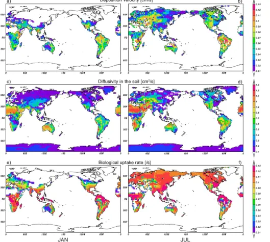
3.1 Deposition velocity and soil uptake of H₂

15

The distribution of the calculated surface deposition velocity of H2, the diffusivity in the soil, and the uptake rate of enzyme activity for January and July are shown in Fig. 1. The globally-averaged deposition velocity over the land surface is 0.33×10−2cm s−1 for the period 1997–2005. The simulated deposition velocity shows a clear geograph-ical distribution and temporal variation. For regions north of 45◦N, a large seasonal

20

change in the deposition velocity can be seen. During the winter, snow cover sup-presses the soil absorption. Furthermore, the decrease of the biological activity by low temperature reduces the rate of deposition. Although the enzyme activity is still maintained near the freezing point, the biological activity in areas like Siberia stops when the soil temperature falls below−25◦C because freezing of soil moisture also

re-25

(14)

ACPD

11, 4059–4103, 2011

H. Yashiro et al.

Title Page

Tables Figures

◭ ◮

Back Close

Full Screen / Esc

Discussion

P

a

per

|

Dis

cussion

P

a

per

|

Discussion

P

a

per

|

Discussio

n

P

a

per

|

deposition velocity starts to increase and the uptake region rapidly expands to north of 50◦N as soil temperature increases and ground snow melts. The deposition velocity in this region reaches a maximum during July and August, and then starts to decrease with the coming of the autumn and winter seasons. In several parts of the region north of 45◦N, the increase in the deposition velocity during the spring and summer is

inter-5

rupted by increases in the soil moisture caused by spring snowmelt and melting soil ice in summer, reducing gas diff_{usivity in the soil.}

In the latitude zone around 30◦N, the temperature is suffi_{ciently high for} en-zyme/bacteria to be active through the year and the soil moisture becomes more im-portant in controlling the deposition velocity. In a desert area, the deposition velocity

10

is near zero because of the near absence of biological activities. The semi-arid region like Central Asia or the central part of North American continent shows larger deposi-tion velocity during the winter than during the summer. Dryness makes diff_{usion in the} soil more effi_{cient in taking H}

2 in this area. However, for intensely high temperature and dryness in the summer, the biological activity becomes weaker and soil uptake is

15

suppressed. The temperate and humid areas such as south China and the southeast-ern part of North America have neither water stress nor high temperature stress, but the high soil moisture suppresses the gas diff_{usion in the soil.}

The seasonal variation in the deposition velocity in the tropics and on the Southern Hemisphere has a smaller amplitude. The factor that has a major influence on the

20

deposition velocity in regions 20◦N to 30◦S is the amount of soil moisture; therefore, the spatial change in the deposition strength is connected with the shift between the rainy and dry seasons. Southern high latitude regions do not make significant contributions to the H2uptake because of the small soil surface area, and needless to say, Antarctica is mostly covered by snow and exhibits almost no deposition.

25

(15)

ACPD

11, 4059–4103, 2011

H. Yashiro et al.

Title Page

Tables Figures

◭ ◮

Back Close

Full Screen / Esc

Discussion

P

a

per

|

Dis

cussion

P

a

per

|

Discussion

P

a

per

|

Discussio

n

P

a

per

|

a rough comparison if the point observation is representative of a larger region. Conrad and Seiler (1980) conducted a year-round observation on the grassland near Mainz, Germany from 1978 to 1979. They reported a seasonal variation in the deposition velocity in the range of 2.6 to 8.8_×10−2cm s−1with a maximum between May and Oc-tober and a minimum between December and February. Similar results were obtained

5

from observations made at grasslands or cultivated lands near their site. In order to compare our model value with their observed value, we choose a grid point that spa-tially corresponds nearly to their cultivated land. For the period between November and April, the simulated deposition velocity of ∼5×10−2cm s−1 agrees with the ob-servational results. During the warm season, the calculated deposition velocity has a

10

large variation in the range of 5–10_×10−2cm s−1 that is associated with the diurnal variation in soil moisture and is comparable with the range of observed values. The deposition velocity observed by Smith-Downey et al. (2006) for the desert shrub of Southern California showed a steep seasonal change. The model is able to capture a similar variation in the semi-arid ecosystem region of the southwestern North America.

15

Both the observed and modeled deposition velocities reach a maximum in early spring with a value of_∼9_×10−2cm s−1, falling thereafter to a value of 2–4_×10−2cm s−1 in June. The rapid decrease is caused by the water stress on the biological activity. In the northern high-latitudes, the observation at a forest site in Finland by Lallo et al. (2006) showed low deposition velocity values (0–4_×10−2cm s−1) in winter and high

20

values (4–7×10−2cm s−1) in snow-free seasons. Our model simulation agrees rela-tively well with the observation, producing a seasonal cycle with an amplitude range of 0–6_×10−2cm s−1. Yonemura et al. (2000b) performed a year-round observation in Asian region. They showed the deposition velocity in the range of 0–10×10−2cm s−1 at the arable field in Japan. However, the model did not capture the seasonal cycle with

25

(16)

ACPD

11, 4059–4103, 2011

H. Yashiro et al.

Title Page

Tables Figures

◭ ◮

Back Close

Full Screen / Esc

Discussion

P

a

per

|

Dis

cussion

P

a

per

|

Discussion

P

a

per

|

Discussio

n

P

a

per

|

to decrease and reaches a value of∼5 Tg yr−1in January. From March to May, a rapid increase of the flux is seen. In the latitude between 15◦N and 45◦N (LNH), the flux remains relatively high throughout the year, increasing from 15 Tg yr−1in February to 20 Tg yr−1in May, and then decreasing gradually thereafter to December. In the tropics (TP), the flux shows almost constant value of 15 Tg yr−1 during the year. In latitudes

5

between 15◦S and 45◦S (LSH), the flux has small seasonal variation. The maximum and minimum values are 11 and 10 Tg yr−1in austral winter and summer, respectively. Almost no uptake is seen south of 45◦S due to the lack of snow-free land surface. In LNH and LSH, variation in the soil moisture is the dominant factor that governs the deposition velocity and the soil uptake. The soil moisture is controlled by rainfall

10

associated with synoptic systems, producing relatively large day-to-day variations in the uptake flux.

3.2 Comparison with the observed H2concentration

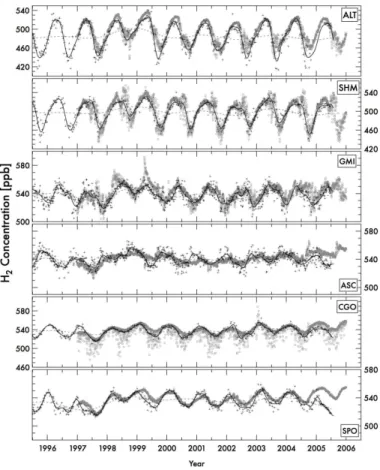
We compare the simulated H2 concentration with the observation obtained from the NOAA/Earth System Research Laboratory (ESRL) network. The summary of

model-15

observation comparisons is given in Table 1 with an explanation of the abbreviated name of each station. The time series of observed and calculated H2concentration for 10 selected stations are shown in Fig. 3. The observed values of some sites indicate a large decrease in concentration from 1991 to 1993 (not shown). Previous studies on CH4and CO pointed to the fact that the variation during this period could be partly

at-20

tributable to the eff_{ects of the Mt. Pinatubo eruption in June 1991. Our model does not} consider the eff_{ect of Mt. Pinatubo and no large inter-annual variation is reproduced by} the model for this period. Furthermore, our model uses the climatology for the biomass burning emission before 1996, resulting in some discrepancies with the observation. We therefore we focus our comparison for the period between 1997 and 2005. To

ex-25

(17)

ACPD

11, 4059–4103, 2011

H. Yashiro et al.

Title Page

Tables Figures

◭ ◮

Back Close

Full Screen / Esc

Discussion

P

a

per

|

Dis

cussion

P

a

per

|

Discussion

P

a

per

|

Discussio

n

P

a

per

|

In general, the model reproduces the observed H2concentration. From Table 1, the overall averaged comparison bias is 0.2%. Averaged value of the Pearson’s moment correlations for the daily mean data at many stations is 0.75. (Comparisons using the monthly mean values show better correlations.) But several stations show noticeably discrepancy in the averaged concentration and/or in correlation coeffi_{cient. Take}

Tu-5

tuila, American Samoa (SMO) for example. The calculated concentration for SMO by the model agrees with the lower concentration values observed during the period 1997 to 2002. After 2003, the observed and simulated concentrations agree relatively well. There are no large, strong sources of H2 near the SMO station and the concentration level in the free troposphere is below 600 ppb, leading to the possibility of certain

lo-10

cal contamination. The result for the station of Tae-ahn Peninsula, Republic of Korea (TAP) shows less agreement in the statistical comparison, likely due to the eff_{ect of} strong local emission.

For Cape Grim, Australia (CGO), simulated values show relatively low and the time series is characterized by spikes of low value, in disagreement with the observation.

15

This diff_{erence is likely caused by the selective sampling procedure employed at this} station in an eff_{ort to obtain “background” concentration levels. Since the sampling} air is selected by using the wind direction to collect maritime air, the air mass arriving from the Australian Continent side is removed. The H2concentration of the air mass, which passed over the Australian Continent, will be lower than the oceanic air mass

20

because of the strong soil uptake. When the same selection procedure is applied to the model result, the low values in the time series at CGO are removed. In Table 1, the comparison with observed and calculated value is obtained by extracting only the observed day, showing good agreement for CGO. Comparisons with other stations are discussed below.

25

3.2.1 Seasonal cycles

(18)

ACPD

11, 4059–4103, 2011

H. Yashiro et al.

Title Page

Tables Figures

◭ ◮

Back Close

Full Screen / Esc

Discussion

P

a

per

|

Dis

cussion

P

a

per

|

Discussion

P

a

per

|

Discussio

n

P

a

per

|

are shown in Fig. 5. Previous observational and model studies have shown that the amplitudes of the seasonal cycle are large in northern high latitudes and decrease towards the tropics. The amplitudes in the southern extra-tropics are slightly higher than those in the tropics, but smaller than those of northern extra-tropics. The upper right panel of Fig. 5 shows that the model reproduces the amplitude distribution

rel-5

atively well, demonstrating that the latitudinal distribution of the seasonal minimum is the major contributor to the north-south gradient.

For regions south of 30◦S, the phase and amplitude of the seasonal variation are similar between the stations, with maximum and minimum occurring in austral sum-mer and winter, respectively. Since the regional contrast of sources and sinks is small

10

and the lifetime is longer than the timescale of transport and mixing, the H₂ concen-tration is well mixed. The homogeneous distribution also results in smaller synoptic variation (see the result of South Pole (SPO) in Fig. 4), expect at CGO for reasons discussed above. Novelli et al. (1999) and Hauglustaine and Ehhalt (2002) pointed out that the main influencing factor of the seasonal cycle in the Southern Hemisphere is

15

the biomass burning. On the other hand, based on their airborne observations of H2 and itsδD ratio, Rhee et al. (2006) noted that the variation in the chemical production is a dominant factor. For CO, seasonal maximums appear during the austral spring in southern high latitudes and are highly connected to the timing of maximum biomass burning emissions in Southern Africa and Southern America. But the seasonal

maxi-20

mums of H₂ occur later than those of CO. In the Southern Hemisphere, the seasonal maximum and minimum of net chemical production appear in austral summer and win-ter, respectively, and the phasing of the H2 seasonal cycle is linked to this rather than the variation in the biomass burning activities. We conclude that the net chemical pro-duction is the more dominant process influencing the H2seasonal cycle in the southern

25

(19)

ACPD

11, 4059–4103, 2011

H. Yashiro et al.

Title Page

Tables Figures

◭ ◮

Back Close

Full Screen / Esc

Discussion

P

a

per

|

Dis

cussion

P

a

per

|

Discussion

P

a

per

|

Discussio

n

P

a

per

|

month later than the observation. Since the emission magnitude from biomass burning adopted in our model is smaller than the previous model studies, the timing of seasonal maximum in our model could be caused by the lack of biomass burning emission.

The stations in the tropics and southern low latitudes such as Ascension Island, UK (ASC, in Fig. 4) and Mahe Island, Seychelles (SEY), show relatively small

sea-5

sonal variation but are characterized by two peaks in spring and autumn with one large seasonal minimum between July and August. The model results capture the pattern well and suggest that the biomass burning in the northern and southern subtropics contribute to the peak in the spring and autumn, respectively. The active region of biomass burning alternates between the hemispheres around the equator in

associ-10

ation with the timing of dry and wet season. The timing of the seasonal minimum is associated with the enhanced inflow of air from the Northern Hemisphere with low H2 concentration, amplified by the strong soil uptake in the tropics.

The occurrence dates of the maximum and minimum are quite diff_{erent between the} Northern Hemisphere and the Southern Hemisphere (see Fig. 4). Around 30◦N, many

15

stations show seasonal maximums occurring between June and July. The seasonal minimums appear during the period from October to December. The seasonal varia-tion in this region is a result of a complicated combinavaria-tion of source/sink change; net chemical production in the atmosphere, oceanic emission, biomass burning, and soil uptake. Variation in large-scale transport also contributes to the observed variation.

20

In general, the model reproduces well the values of maximum and minimum at many stations, but causes both maximum and minimum to occur one to two months earlier. For inland sites near arid regions, such as Wendover, United States (UTA, in Fig. 4), Ulaan Uul, Mongolia (UUM, in Fig. 4), and Sary Taukum, Kazakhstan (KZD), large discrepancies between model and observation can be seen. Model results at these

25

(20)

ACPD

11, 4059–4103, 2011

H. Yashiro et al.

Title Page

Tables Figures

◭ ◮

Back Close

Full Screen / Esc

Discussion

P

a

per

|

Dis

cussion

P

a

per

|

Discussion

P

a

per

|

Discussio

n

P

a

per

|

water stress. It is possible that the coarseness of the model grid fails to capture the real heterogeneity of the soil types in the semi-arid regions and thus is unable to capture the strong local uptake.

For regions north of 45◦N, the seasonal maximum appears in the late spring and the minimum at the beginning of the autumn at every station. The amplitude of the

5

seasonal cycle increases poleward, reaching about 70 ppb at Alert, Canada (ALT, in Fig. 4). This latitudinal change in the amplitude is related to the poleward decrease in the value of the seasonal minimum. The model results agree well in the timing of the occurrence of the seasonal maximum/minimum, as well as in the maximum value, but slightly underestimate the seasonal minimum. This problem is connected with the

10

representation of the physical property of the uppermost soil. There still is a great deal of uncertainty associated with the air ratio at the soil surface, which is influenced by the melting of frozen soil in their summer. In addition, it is conceivable that the biologically inactive layer is thinner in this region. The soil temperature in this region remains relatively low even in the summer and this can decrease the thickness of the

15

inactive layer. At stations along the Pacific rim, such as Shemya Island, United States (SHM, in Fig. 4) and Cold Bay, United States (CBA), the concentrations decrease with large day-to-day variation from summer to autumn. These variations are related to the variation in the transport of maritime and continental air masses with diff_{erent H}₂ concentration caused by enhanced summer emission of H₂by the ocean and by strong

20

soil uptake on the continent.

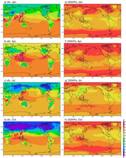
3.2.2 Global distribution, budgets and trend of H₂

The global distributions of simulated H2 concentration at the surface and 250 hPa in January, April, July, and October are shown in Fig. 6. Zonal averages of H₂distribution for the same months are shown in Fig. 7. The horizontal and vertical distributions of

25

(21)

ACPD

11, 4059–4103, 2011

H. Yashiro et al.

Title Page

Tables Figures

◭ ◮

Back Close

Full Screen / Esc

Discussion

P

a

per

|

Dis

cussion

P

a

per

|

Discussion

P

a

per

|

Discussio

n

P

a

per

|

near the ocean surface during the austral summer at this latitudinal band is 5–10 ppb higher than in the upper troposphere, due mainly to the presence of oceanic sources. In contrast, the concentration over the land surface indicates values 10–30 ppb lower than those in the free troposphere due to the soil uptake. In the tropical region, the oceanic emission and net chemical production of H₂are relatively high throughout the

5

year. In addition, biomass burning emits large amounts of H2, especially during boreal spring and autumn, at least partially off_{setting the large soil uptake.}

The tropics and subtropics are regions where emissions of biogenic NMVOCs are strong and cumulus convection is active. This results in a strong vertical transport to the upper troposphere of NMVOCs and NOxfrom both the biogenic and pyrogenic sources

10

at the surface. Enhanced chemical reactions result in a higher production of H₂at the 200–300 hPa levels, compared to the situation in the lower free troposphere. However, vertical transport of low-H2 air mass affected by the soil uptake results in a region of relatively low H₂concentration in the uppermost troposphere of the subtropics, mainly over the continents.

15

The Northern Hemisphere shows large seasonally varying vertical gradients in H2, with the maximum occurring in boreal spring and autumn, respectively. The lowest con-centration is seen near the surface of northern high latitudes, with low concon-centration areas spreading to the upper troposphere and lower latitudes. The contrast in the con-centration between land and ocean is large in northern mid- and high-latitudes.

Anthro-20

pogenic emissions are strong in areas with large population, such as North America, Europe, and China, resulting in high H2concentrations, especially over the China and India. In the summer (July, Fig. 6c), we see an area of high H₂concentration over East Asia and Southeast Asia spreading to the western Pacific and farther east along the subtropical Pacific with slightly lower concentration, indicating an enhanced transport

25

of oceanic air mass associated with the Asian monsoon.

(22)

ACPD

11, 4059–4103, 2011

H. Yashiro et al.

Title Page

Tables Figures

◭ ◮

Back Close

Full Screen / Esc

Discussion

P

a

per

|

Dis

cussion

P

a

per

|

Discussion

P

a

per

|

Discussio

n

P

a

per

|

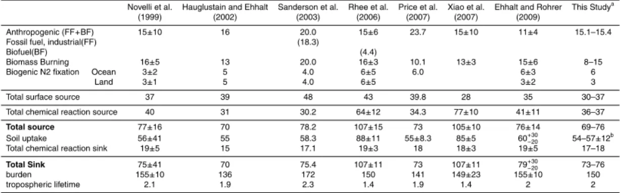
37 Tg yr−1and 17–18 Tg yr−1, with respective average values of 36.6±0.3 Tg yr−1and 18.1_±0.2 Tg yr−1. The annual total flux of soil uptake has a range of 54–57 Tg yr−1, with an average value of 56.2_±0.9 Tg yr−1. These values correspond relatively well with values obtained by other forward models (Hauglestain and Ehhalt, 2002; Sander-son et al., 2003; Price et al., 2007). However, Rhee et al. (2006) and Xiao et al. (2007)

5

reported a larger estimate of soil uptake flux (88 and 85 Tg yr−1, respectively) and chemical production (64 and 77 Tg yr−1, respectively). The larger production values re-sulted from the assumption of larger production from the oxidation of NMVOCs. Ehhalt and Rohrer (2009) pointed out that the estimate of the soil uptake has large uncer-tainty, and advocated 55+_30/₋_{20 Tg yr}−1_{, which brings it closer to our results. The}

10

estimate by Rhee et al. (2006) was based on a simplified calculation involving the seasonal variation of the concentration and isotope ratio of H₂in the free northern mid-latitude troposphere. They assumed that the Northern Hemisphere troposphere is well mixed and that soil uptake and net chemical production contribute uniformly in vertical. However, as noted above, the footprint of the soil uptake in the upper troposphere is

15

mediated by the vertical convective transport in the tropics and subtropics, resulting in temporal and spatial heterogeneity in the H2 concentration. Furthermore, a global simulation of H₂ isotope by Price et al. (2007) showed that the ground observations ofδDcould be explained by a smaller H2 soil uptake than that estimated by Rhee et al. (2006). Xiao et al. (2007), on the other hand, used an inversion method with a 2-D

20

multi-box model employing relatively few observations to constrain their results. One of the problems with this approach is that the seasonal variation of H2near the surface is quite diff_{erent over the ocean and land, causing the 2-D inversion to be sensitive to} the station location. When many observation points near the continent are used, the influence of soil uptake may be overestimated. In our model, the soil uptake is

calcu-25

(23)

ACPD

11, 4059–4103, 2011

H. Yashiro et al.

Title Page

Tables Figures

◭ ◮

Back Close

Full Screen / Esc

Discussion

P

a

per

|

Dis

cussion

P

a

per

|

Discussion

P

a

per

|

Discussio

n

P

a

per

|

Novelli et al. (1999) showed that tropospheric H2does not display a clear increasing or decreasing trend after 1995, in agreement with our results shown in Fig. 3. Globally averaged source/sink H2 anomalies and the corresponding tropospheric burden are shown in Fig. 8. Superimposed on the gradual total emission increase due mainly to growing anthropogenic emissions, there is a noticeable inter-annual variability caused

5

by emissions from large biomass burnings. Especially the emission from the Indone-sian fires during 1997–1998, and from the forest fires in Siberia in 1998 are significant. In contrast, year 2000 saw very little biomass burning. We also see inter-annual vari-ability in the soil uptake flux of H2, offsetting the emissions. The net total emission from the surface, along with the chemical production, of H2 is reflected in the tropospheric

10

burden of H₂, which shows a slight increasing (but not significant) trend from 2002 to 2005. The biomass burning in 1998 brought a temporary increase in the tropospheric burden but recovered in about two years. The observed H2 concentration also shows a corresponding peak during 1997–1998 (Fig. 3). The summertime increase in 1998 was observed at nearly all stations and the model is found to reproduce it relatively

15

well. Both the chemical production and loss show an increasing trend. It is possible that this increase is related to an increase in the methane oxidation rate caused by an increase in global temperature, and/or is related to an increase in OH radical caused by an increase in the water vapor. However, the amount of change is very small compared to changes in the surface emission.

20

The soil uptake not only responds to an increase in atmospheric concentration but also to changes in soil temperature and moisture. The long-term variations in the total and average values of simulated soil uptake flux, deposition velocity, and soil moisture in four latitude bands are shown in Fig. 9. They are obtained by applying the curve fitting method of Nakazawa et al. (1997). From the figure, both the soil uptake

25

(24)

ACPD

11, 4059–4103, 2011

H. Yashiro et al.

Title Page

Tables Figures

◭ ◮

Back Close

Full Screen / Esc

Discussion

P

a

per

|

Dis

cussion

P

a

per

|

Discussion

P

a

per

|

Discussio

n

P

a

per

|

Ropelewski and Halpert (1987) (also shown in Fig. 9), the increase in soil moisture in 2000 is linked to an increase in precipitation around Indonesia caused by a La Nina event. Although an increase in precipitation on land in a tropical region decreases the soil uptake of H2, it actually reduces the frequency of biomass burning in the same area. This balance between the reduced emission and reduced soil uptake results in

5

very little change in atmospheric H2, as was the case in the tropics in 2000 (Fig. 2).

3.3 Possible uncertainty of soil uptake flux

In the soil diff_{usion model used in this study, the factors that produce uncertainties in} the soil estimate are the diff_{usion coe}ffi_{cient in soil, the degree of biological activity, and} the inactive layer thickness. The diff_{usivity and the biological activity are determined by}

10

the air ratio in the soil, soil moisture, and soil temperature. Prediction errors of these variables are expected to aff_{ect the deposition velocity of H}

2. The good agreement between our model result and the observations gives indirect support to the ability of our model to reproduce relatively well the soil moisture and temperature in general. Furthermore, inter-annual variations in the soil variables do not appear to produce

15

large variations in the global soil uptake, thus having minimal impact on the budget of tropospheric H2. The factor that produces greater uncertainty is associated with the specification of soil properties, such as the ratio of soil surface area to the aerial volume, and the ratio of the volume of solids. The change in the physical structure of the soil within the first several centimeters from the surface is large. This demands

20

a better and more detailed distribution of soil variables with fine vertical resolution in the top soil layer. In this study, the correction of∼0.2 g g−1 is uniformly applied to the air ratio in consideration of vertical ununiformity of the air ratio at the uppermost layer. However, this correction is not enough to capture a sharp change of the air ratio near the surface.

25

(25)

ACPD

11, 4059–4103, 2011

H. Yashiro et al.

Title Page

Tables Figures

◭ ◮

Back Close

Full Screen / Esc

Discussion

P

a

per

|

Dis

cussion

P

a

per

|

Discussion

P

a

per

|

Discussio

n

P

a

per

|

the deposition velocity around the observation stations. Semi-arid regions have a large potential for H2 uptake but this uptake is prevented by the dryness. That is, the soil uptake of H2in a semi-arid region is highly sensitive to change in the vertical distribution of soil moisture. A better representation of arable fields is also important in improving the estimation of global H2 uptake by the soil. Although we do not carry out model

5

verification in regards to the H2 uptake by the arable land, we realize that seasonal changes in the surface condition and in the vertical soil properties are significant and will likely have a large impact on the soil uptake estimate. Large variations in soil properties and the inactive layer thickness caused by strong sunlight can take place over a short time period.

10

The global distribution of the inactive layer thickness is practically not known. The formation of the inactive layer is mainly due to the irreversible destruction of enzymes or bacteria near the surface soil. Thus, the temporal change in the inactive layer thickness is influenced not only by the physical stress such as extreme heating and drying but also by the recovery/redistribution rate of microbes and enzymes. Figure 10 shows

15

the sensitivity of the annually averaged deposition velocity on land to the thickness of the inactive layer δ. The figure shows a near 50% diff_{erence in the deposition} velocity betweenδ=_{0 and}_δ=₁_._{0 cm. This is equivalent to 25–30 Tg yr}−1_diff_{erence in} global soil uptake, which is not negligible, considering the size of the global H2budget. In this study, δ=₀_._{7 cm was adopted, because it optimizes the agreement with the}

20

observation. With the assumption thatδ has a range of 0.3 to 1.4 cm, we obtain an uncertainty of ±20% for the estimated deposition velocity over the land which gives ±12 Tg yr−1uncertainty for a global soil uptake estimate. Although the assumed range ofδis consistent with those estimated by other investigators (Yonemura et al., 2000b; Shmitt et al., 2009), we need much more observations to obtain a more realistic idea

25

(26)

ACPD

11, 4059–4103, 2011

H. Yashiro et al.

Title Page

Tables Figures

◭ ◮

Back Close

Full Screen / Esc

Discussion

P

a

per

|

Dis

cussion

P

a

per

|

Discussion

P

a

per

|

Discussio

n

P

a

per

|

4 Conclusions

We have conducted a global simulation of tropospheric H₂ concentrations and eval-uated its uptake by land using the global chemical transport model, CHASER. The soil diff_{usion model, which has an inactive and active layer of biological consumption} rate, is incorporated into the dry deposition scheme. The variation in the soil diff_usivity

5

and biological activity in the soil are calculated as a function of soil temperature and moisture, which are calculated as prognostic variables in the land process module of the model. The model results of the regional distribution and seasonal variation of the H2deposition velocity agree relatively well with the observed values obtained by other investigators.

10

A large seasonal variation in the deposition velocity corresponding to changes in soil temperature and snowfall is seen in the northern high latitudes. In the mid-latitudes of both hemispheres and the tropics, we can identify two regional types where (1) bio-genic uptake is active because of the warm climate, but the wet environment counters diff_{usion to the soil, and (2) biological activity becomes weaker due to high temperature}

15

and dryness, but the dry climate makes the transportation in the soil more effi_{cient. The} strength of soil uptake is closely related to the water and heat budget in each region.

The H2concentration calculated by the model reproduces relatively well the concen-tration observed at the NOAA stations. The seasonal variation of the concenconcen-tration in the Southern Hemisphere is mainly due to the net chemical production in austral

sum-20

mer and the inflow of the relatively low H2air mass from the north following the north-south transport in austral winter. The vertical and horizontal gradients are small in the Southern Hemisphere. In the tropics, both the net chemical production and the soil uptake are high through the year and the impact of biomass burning is superimposed during January and September. Furthermore, in the tropical region, active cumulus

25

(27)

ACPD

11, 4059–4103, 2011

H. Yashiro et al.

Title Page

Tables Figures

◭ ◮

Back Close

Full Screen / Esc

Discussion

P

a

per

|

Dis

cussion

P

a

per

|

Discussion

P

a

per

|

Discussio

n

P

a

per

|

to the H2 variation in the Northern Hemisphere. During the boreal summer, a strong uptake by the soil surface produces a large vertical gradient, land-sea gradient, and latitudinal gradient in the H2concentration.

For our simulation period of 1997 to 2005, the average tropospheric burden and lifetime are found to be 150 Tg and 2.0 year, respectively. The annual total amount of

5

chemical production, chemical loss, and soil uptake are 36, 18, 56 Tg yr−1, respectively. The budget calculated from our simulation agrees with the lower end of the estimated values obtained by previous forward model studies.

Our model is able to reproduce the overall inter-annual variation observed during the period 1997–2005. Large H2 concentration peaks caused by large biomass burning

10

in Indonesia and Siberia were observed in 1997 and 1998, respectively at nearly all stations. Our model is able to successfully reproduce these peaks.

Although the anthropogenic emission has been increasing over the last several years, the tropospheric H₂ concentration shows no significant long-term trend. Our model result shows that the soil uptake flux changes in the direction that off_{sets the}

in-15

crease in H2emission to the atmosphere. The simulated H2deposition velocity shows a small trend and inter-annual variation. We conclude that the recent decadal climate change has had very little impact on the H2concentration.

The global soil uptake flux of H2 obtained by our model succeeds in reproducing the tropospheric H2concentration and its seasonal variation observed at many of the

20

stations distributed throughout the world. However, in regions where one has a strong H2 uptake, uncertainties in both uptake flux and atmospheric concentration are still large. In order to improve the estimate of the soil uptake flux and to reproduce/predict the present/future concentration of H₂in the atmosphere, it is necessary to develop a detailed knowledge of the vertical structure of physical soil properties and the response

25