Atmospheric speciated mercury concentrations on an island between China and Korea: sources and transport pathways

(1)

ACPD

15, 32931–32966, 2015

Atmospheric speciated mercury

concentrations

G.-S. Lee et al.

Title Page

Abstract Introduction

Conclusions References

Tables Figures

◭ ◮

Back Close

Full Screen / Esc

Printer-friendly Version Interactive Discussion

Discussion

P

a

per

|

Discussion

P

a

per

|

Discussion

P

a

per

|

Discussion

P

a

per

|

Atmos. Chem. Phys. Discuss., 15, 32931–32966, 2015 www.atmos-chem-phys-discuss.net/15/32931/2015/ doi:10.5194/acpd-15-32931-2015

This discussion paper is/has been under review for the journal Atmospheric Chemistry and Physics (ACP). Please refer to the corresponding final paper in ACP if available.

Atmospheric speciated mercury

concentrations on an island between

China and Korea: sources and transport

pathways

G.-S. Lee1, P.-R. Kim1, Y.-J. Han1, T. M. Holsen2, Y.-S. Seo3,4, and S.-M. Yi3

1

Department of Environmental Science, College of Natural Science, Kangwon National University, 1 Kangwondaehak-gil, Chuncheon, Kangwon-do, 200-701, Republic of Korea 2

Department of Civil and Environmental Engineering, Clarkson University, 8 Clarkson Ave., Potsdam, NY 13699-5710, USA

3

Department of Environmental Health, Graduate School of Public Health, Seoul National University, Gwanak-ro, Gwanak-gu, Seoul 151-742, Republic of Korea

4

Institute of Health and Environment, Seoul National University, 1 Gwanak-ro, Gwanak-gu, Seoul 151-742, Republic of Korea

Received: 20 October 2015 – Accepted: 7 November 2015 – Published: 24 November 2015

Correspondence to: Y.-J. Han (youngji@kangwon.ac.kr)

(2)

ACPD

15, 32931–32966, 2015

concentrations

G.-S. Lee et al.

Title Page

Tables Figures

◭ ◮

Back Close

Full Screen / Esc

Discussion

P

a

per

|

Discussion

P

a

per

|

Discussion

P

a

per

|

Discussion

P

a

per

|

Abstract

As a global pollutant, mercury (Hg) is of particular concern in East Asia where an-thropogenic emissions are the largest. In this study, speciated Hg concentrations were measured in the western most island in Korea, located between China and the Korean mainland to identify the importance of local, regional and distant Hg sources. Various

5

tools including correlations with other pollutants, conditional probability function, and back-trajectory based analysis consistently indicated that Korean sources were impor-tant for gaseous oxidized mercury (GOM) whereas, for total gaseous mercury (TGM) and particulate bound mercury (PBM), long-range and regional transport were also important. A trajectory cluster based approach considering both Hg concentration and

10

the fraction of time each cluster was impacting the site was developed to quantify the effect of Korean sources and out-of-Korean source. This analysis suggests that Ko-rean sources contributed approximately 55 % of the GOM and PBM while there were approximately equal contributions from Korean and out-of-Korean sources for the TGM measured at the site. The ratio of GOM/PBM decreased when the site was impacted

15

by long-range transport, suggesting that this ratio may be a useful tool for identifying the relative significance of local sources vs. long-range transport. The secondary for-mation of PBM through gas-particle partitioning with GOM was found to be important at low temperatures and high relative humidity.

1 Introduction

20

Mercury (Hg) is the only metal that exists as a liquid at standard conditions (US EPA, 1997) which results in it having a significant vapor pressure and presence in the at-mosphere. In the atmosphere, Hg generally does not constitute a direct public health risk at the level of exposure usually found (Driscoll et al., 2007). However, once Hg is deposited into aquatic systems, it can be transformed into methyl-mercury (MeHg)

25

(3)

ACPD

15, 32931–32966, 2015

concentrations

G.-S. Lee et al.

Title Page

Tables Figures

◭ ◮

Back Close

Full Screen / Esc

Discussion

P

a

per

|

Discussion

P

a

per

|

Discussion

P

a

per

|

Discussion

P

a

per

|

1995). Many studies show that one of the major sources of MeHg in aquatic system is atmospheric deposition of inorganic Hg (Landis and Keeler, 2002; Mason et al., 1997). Atmospheric mercury exists in three major inorganic forms, including gaseous ele-mental mercury (GEM, Hg0), gaseous oxidized mercury (GOM, Hg2+) and particulate bound mercury (PBM, Hg(p)). The sum of the GEM and GOM is often called as total

5

gaseous mercury (TGM). Due to its high water solubility and deposition velocity, GOM has short atmospheric residence times (∼day) and, consequently, its ambient

con-centration is mainly affected by local sources. In contrast, GEM, which comprises more than 95 % of the total Hg in ambient air, can be transported long distances because it is relatively inert and has low water solubility and deposition velocity (Lin and Pehkonen,

10

1999). The residence time of PBM is dependent on the size of associated particles, but generally, it has been assumed to be a few days (Fang et al., 2012; Zhang et al., 2001). Measurements of GOM and PBM are challenging and uncertain due to their extremely low concentrations and complex chemical reactivity, and because their chemical forms are not actually known (Pirrone et al., 2013). In most studies, GOM and PBM have

15

operational definitions for the mercury species collected by a KCl coated denuder and by a quartz filter downstream of a KCl denuder, respectively.

In the atmosphere, Hg species can be interconverted through various redox reac-tions. It is known that GOM can be produced by homogeneous and heterogeneous re-actions of GEM with O₃, OH, and Br/BrO (Hedgecock and Pirrone, 2004; Obrist et al.,

20

2011), but there is no consensus on which oxidants are most important. GEM can also be formed through reduction of GOM predominantly in cloud water (Subir et al., 2011, 2012). GOM can also be converted to PBM through gas-particle partitioning, with the partition coefficient,Kp, inversely correlated with temperature and positively correlated

with particle surface area (Lyman and Keeler, 2005; Liu et al., 2010). Since GEM makes

25

(4)

ACPD

15, 32931–32966, 2015

concentrations

G.-S. Lee et al.

Title Page

Tables Figures

◭ ◮

Back Close

Full Screen / Esc

Discussion

P

a

per

|

Discussion

P

a

per

|

Discussion

P

a

per

|

Discussion

P

a

per

|

The region of largest anthropogenic Hg emissions is East and Southeast Asia, con-tributing 39.7 % of the total anthropogenic emissions (UNEP, 2013). In Korea, atmo-spheric Hg emissions have generally decreased since 1990. However, Hg levels in Korea are likely to be highly susceptible to Chinese emissions because China alone accounts for about one third of the global total (UNEP, 2013) and Korea is situated just

5

west (and generally downwind) of China. According to the recent studies, Hg concen-trations in blood of Koreans are more than 4–8 times higher than those found in US and Germany, and approximately 26 % of Koreans have higher blood mercury concen-trations than a USA guideline level (http://envhealth.nier.go.kr), indicating that there is an urgent need to identify the Hg sources and pathways controlling Hg concentrations

10

in Korea.

This study was designed to identify the contribution of various Hg sources including direct emissions from anthropogenic and natural sources and indirect secondary for-mation processes to atmospheric Hg concentrations in Korea. In order to achieve these objectives, Hg concentrations were measured in the western most island in Korea,

lo-15

cated in between eastern China and the Korean mainland, so that, depending on wind patterns, the e_ffects of Chinese and Korean Hg emissions could be evaluated. Previ-ously, our group qualitatively evaluated the impact of local Korean sources and regional Chinese sources on TGM concentrations at the same sampling site (Lee et al., 2014). However, that work was unable to identify the e_ffect of sources on Hg levels in Korea

20

(5)

ACPD

15, 32931–32966, 2015

concentrations

G.-S. Lee et al.

Title Page

Tables Figures

◭ ◮

Back Close

Full Screen / Esc

Discussion

P

a

per

|

Discussion

P

a

per

|

Discussion

P

a

per

|

Discussion

P

a

per

|

2 Materials and methods

2.1 Site description

TGM, GOM and PBM were measured on the roof of a three-story building on Yonghe-ung Island (YI), the westernmost island in Korea (Fig. 1). YI is a small island located about 15–20 km west from mainland Korea with a population of 5815. The

Yonghe-5

ung Coal-fired Power Plant (YCPP), located approximately 4.5 km southwest of the sampling site (Fig. 1c), emits about 0.11 t yr−1of Hg. To the east of the sampling site, industrial (the Incheon industrial complex shown as light violet color in Fig. 1b and c) and metropolitan (Seoul shown as a pink color in Fig. 1b and c) areas are located in mainland Korea, and, in the southern direction, there are three large coal fired power

10

plants (Fig. 1b). The Hg emission rate of anthropogenic sources in Korea was esti-mated to be 8.04 t yr−1in 2010, with cement production being the largest source type (AMAP/UNEP, 2013).

2.2 Sampling and analysis

From January 2013 to August 2014, three atmospheric mercury species: TGM

15

(GEM+GOM), GOM, and PBM (≤2.5 µm) were measured during eight intensive

sam-pling periods (Table 1). TGM concentrations were measured every 5 min using a mer-cury vapor analyzer (Tekran 2537B). This instrument contains two gold cartridges which collect and thermally desorb Hg alternately. Desorbed Hg is quantifed using a cold vapor atomic fluorescence spectrometry (CVAFS). Outdoor air at a flow rate of

20

1.0 L min−1was transported through a 3 m-long heated sampling line (1/4′′OD Teflon) into the analyzer. The Tekran 2537B was automatically calibrated daily using an internal permeation source. Manual injections were also used to evaluate these automated cal-ibrations before each sampling campaign using a saturated mercury vapor standard. The relative percent difference between manual injection and automated calibration

25

(6)

ACPD

15, 32931–32966, 2015

concentrations

G.-S. Lee et al.

Title Page

Tables Figures

◭ ◮

Back Close

Full Screen / Esc

Discussion

P

a

per

|

Discussion

P

a

per

|

Discussion

P

a

per

|

Discussion

P

a

per

|

into the sampling line two times during the study period. TheR2 ranged from 0.9991 to 0.9997 between mass injected and Tekran reported area, and the average relative percent di_fference between the mass injected and the mass calculated was 5.5 %. The method detection limit (0.04 ng m−3) was calculated as three times the standard devia-tion obtained after injecting 1 pg of the mercury vapor seven times. The recovery rate

5

(96±3 %) was obtained by directly injecting Hg vapor into the sampling line between

the sample inlet and the Tekran 2537B in a zero-air stream.

GOM and PBM were collected manually using an annular denuder coated with KCl followed by a quartz filter, respectively, at a flow rate of 10 L min−1. To identify any diurnal variations, all samples were separately collected during the daytime (07:00–

10

19:00 LT) and nighttime (19:00–07:00 LT) except during the 7th sampling period when they were measured every 2 h. The sampling system including an elutriator, an im-pactor, a KCl-coated denuder and a filter pack was housed in a custom-made sam-pling box maintained at 45◦C to prevent hydrolysis of KCl. After sampling, the denuder and quartz filter were thermally desorbed using a tube furnace at 525 and 900◦C,

15

respectively, to convert Hg2+ to Hg0 in a carrier gas of zero air. The heated air was then transported into a Tekran 2537B for quantification. Field blanks for GOM and PBM were collected once for each sampling period, and their average values were 0.23±0.12 pg m−3and 0.25±0.09 pg m−3, respectively.

The sampling methods used in this study are currently the most accepted methods

20

for the measurement of atmospheric GOM and PBM, however there are many studies reporting that these methods are subject to interferences from ozone, water vapor and possibly other compounds (Lyman et al., 2010; Talbot et al., 2011; Jeffet al., 2014; Fin-ley et al., 2013; Gustin et al., 2013; Huang et al., 2013; McClure et al., 2014) although recent side-by-side measurements with two Tekran systems showed good agreement

25

(7)

ACPD

15, 32931–32966, 2015

concentrations

G.-S. Lee et al.

Title Page

Tables Figures

◭ ◮

Back Close

Full Screen / Esc

Discussion

P

a

per

|

Discussion

P

a

per

|

Discussion

P

a

per

|

Discussion

P

a

per

|

Meteorological data including temperature, wind speed, wind direction, relative hu-midity and solar radiation were also measured every 5 min at the sampling site using a meteorological tower (DAVIS Inc weather station, Vintage Pro2TM).

Hourly concentrations of SO2, NO2, CO, O3 and PM10 were obtained from the

na-tional air quality (NAQ) monitoring station (http://www.airkorea.or.kr/) located

approx-5

imately 8 km east from the sampling site. These concentrations were compared with those measured at another national air quality monitoring station located approximately 24 km west of the Hg sampling site, and there were no statistical differences between sites (p value <0.001), indicating that the spatial distribution of these pollutants was relatively uniform across the area.

10

2.3 Backward trajectory and cluster analysis

Three-day backward trajectories were calculated using the NOAA HYSPLIT 4.7 with GDAS (Global Data Assimilation System) meteorological data which supplies 3 h, global 1◦ latitude–longitude datasets of the pressure surface. Hourly 3 day back-trajectories were calculated for each hour of sampling, and the arrival heights of both

15

200 and 500 m were used to describe the local and the regional transport meteorolog-ical pattern, respectively.

The backward trajectories were clustered into groups with similar transport patterns using NOAA HYSPLIT 4.7. This method minimizes the intra-cluster di_fferences among trajectories while maximizing the inter-cluster differences. The clustering of trajectories

20

(8)

ACPD

15, 32931–32966, 2015

concentrations

G.-S. Lee et al.

Title Page

Tables Figures

◭ ◮

Back Close

Full Screen / Esc

Discussion

P

a

per

|

Discussion

P

a

per

|

Discussion

P

a

per

|

Discussion

P

a

per

|

2.4 Conditional Probability Function (CPF)

The conditional probability that a given concentration from given wind direction will ex-ceed a predetermined threshold criterion, was calculated using the following equation.

CPF_∆θ=

m_∆θ

n_∆θ (1)

wherem_∆θ is the number of occurrences from wind sector∆θwhere the concentration

5

is higher than a criterion value, andn_∆θ is the total number of occurrence from this wind sector.

2.5 Potential Source Contribution Function (PSCF)

The PSCF model counts each trajectory segment endpoint that terminates within given grid cell. A high PSCF value signifies a potential source location. The PSCF value was

10

calculated as:

PSCF value=P[Bi j]

P[A_{i j}]=

m_{i j}

n_{i j} (2)

where m_{i j} is the number of endpoints associated with a concentration higher than a criterion value inijth cell, andn_{i j} is total number of endpoints inijth cell. The criterion value was the top 25 % concentration and the cell size of 0.5◦ by 0.5◦ was used for

15

tracing sources. To reduce the uncertainty in a grid cell with a small number of end-points, an arbitrary weight functionW_{i j} was applied when the number of the endpoints in a particular cell was less than three times the average number of endpoints (Nave)

for all cells (Fu et al., 2011; Han et al., 2007; Polissar et al., 2001a, b).

W_{i j}= 

  

1.0 N_{i j}>3Nave

0.70 3Nave> Ni j >1.5Nave

0.40 1.5Nave> Ni j> Nave

0.20 Nave> Ni j



  

(3)

(9)

ACPD

15, 32931–32966, 2015

concentrations

G.-S. Lee et al.

Title Page

Tables Figures

◭ ◮

Back Close

Full Screen / Esc

Discussion

P

a

per

|

Discussion

P

a

per

|

Discussion

P

a

per

|

Discussion

P

a

per

|

3 Results and discussion

3.1 General trends of three Hg species

The average TGM, GOM, and PBM concentrations were 2.8±1.1 ng m−3, 9.8±

9.9 pg m−3, and 10.6±12.0 pg m−3, respectively (Table 1). Since the GOM concentra-tion was much lower than TGM the reported TGM concentraconcentra-tion can be considered

5

a good approximation of the GEM concentration. TGM varied from 0.1 to 18.8 ng m−3; the highest concentration was observed around 2 a.m. on 18 March 2014 (Fig. 2). GOM and PBM concentrations peaked at 50.9 pg m−3during the daytime on 19 March 2014 and 56.5 pg m−3 in the early morning (06:00–08:00 LT) of 28 May 2014, respectively (Fig. 2). The various Hg species did not follow similar concentration patterns although

10

PBM was statistically significantly correlated with TGM (Pearson correlation coefficient,

r=0.235,pvalue=0.03).

The data were grouped into four seasons including spring (March, April, May), sum-mer (June, July, August), fall (September, October, November) and winter (Decem-ber, January, February). Both TGM (ANOVA/Tukey test, p value <0.001) and PBM

15

(pvalue=0.024, Kruska–Wallis test) had the highest concentrations in winter, followed by spring and summer while there was no statistical difference in GOM concentrations among different seasons (pvalue=0.288, Kruskal–Wallis test) (Fig. 3). Observed TGM concentrations were substantially lower than those measured in a suburban and re-mote site in China and metropolitan areas of Korea (Seoul), but higher than at most

20

North American sites and at a rural site of Korea (Chuncheon) (Table 2). GOM and PBM concentrations were in between those typically found at urban locations and at a rural site in Korea and were much lower than those typically measured in China.

The TGM concentration varied diurnally, generally showing morning maximums (07:00–12:00 LT) and minimums during the nighttime. In urban areas, TGM

concen-25

(10)

ACPD

15, 32931–32966, 2015

concentrations

G.-S. Lee et al.

Title Page

Tables Figures

◭ ◮

Back Close

Full Screen / Esc

Discussion

P

a

per

|

Discussion

P

a

per

|

Discussion

P

a

per

|

Discussion

P

a

per

|

peaks have been observed in rural and remote areas, likely due to increased volatilized of Hg0from natural sources (Choi et al., 2008; Cheng et al., 2014). Overall these re-sults suggest that TGM concentrations at this site are elevated due to the proximity of regional sources and daily variations are controlled by natural emissions from the ocean and soil surfaces.

5

GOM concentrations were the highest in spring (10.7±10.1 pg m−3) and the lowest in summer (6.2±4.9 pg m−3) with statistically insignificant seasonal variation (Fig. 3). The lack of a GOM seasonal variation for could be an indicator of insignificant secondary formation through photochemical oxidation reactions, but it might be also be due to the small sample numbers and/or relatively long sampling duration (12 h). PBM

concen-10

trations did have statistically significant seasonal variations with the highest average concentration in winter (17.8±16.7 pg m−3) and the lowest average concentration in

summer (5.8±4.1 pg m−3) (Fig. 3). Higher PBM concentrations in winter were likely caused by increased biomass burning and residential heating, decreased removal from the atmosphere due to the lower precipitation depth, and/or lower temperatures which

15

favor partitioning to the aerosol phase. Previous studies also often observed the high-est PBM concentrations in winter (Mao et al., 2012; Amos et al., 2012; Lan et al., 2012). In Korea emissions of PBM from anthropogenic sources are much smaller then gaseous emissions (the proportion of GEM, GOM, and PBM released are 64.4, 28.8, and 6.8 %) (Kim et al., 2010). The fact that PBM concentrations are similar to GOM

20

even though significantly less PBM is released suggests that a significant portion of at-mospheric PBM may be due to secondarily formation through gas-particle partitioning. This process is characterized by a partition coefficient,Kp, which is inversely correlated

with temperature (Rutter and Schauer, 2007), possibly causing the distinct seasonal variation in PBM concentrations at the sampling site.

25

The relationship betweenKp, defined as:

Kp=

PBM/PM Hggas

(11)

ACPD

15, 32931–32966, 2015

concentrations

G.-S. Lee et al.

Title Page

Tables Figures

◭ ◮

Back Close

Full Screen / Esc

Discussion

P

a

per

|

Discussion

P

a

per

|

Discussion

P

a

per

|

Discussion

P

a

per

|

where PM represents the particle mass, and Hg_gasis the concentration of gaseous Hg and relative humidity (RH) was examined. RH was included since in recent studiesKp

was found to increase at high relative humidity in colder seasons (Lyman and Keeler, 2005; Liu et al., 2010). Note that the sampling site was located in a coastal area with generally high RH.

5

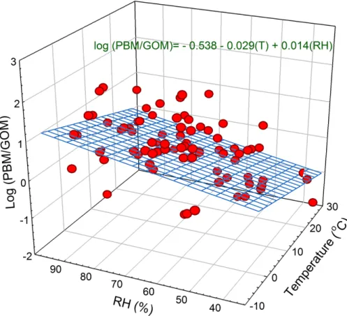
Some previous studies suggested that all gaseous mercury species including Hg0 may deposit on particles (Xiu et al., 2005, 2009); however, others suggested that the gas-particle partitioning of GOM occurred but assumed that the adsorption of Hg0on particles was negligible due to its high vapor pressure (Amos et al., 2012; Rutter and Schauer, 2007). Consistent with this hypothesis, we found a statistically significant

mul-10

tiple linear relationship between the ratio of PBM/GOM with temperature and relative humidity (Fig. 4):

log(PBM/GOM)=−538−0.029(T)+0.014(RH) (5) whereT and RH indicate atmospheric temperature (◦C) and relative humidity (%), re-spectively. The multiple linear equation fit the data well (R=0.49, p value <0.001),

15

and both variables of temperature and relative humidity were statistically significant (p value<0.001). When the temperature was used as a single independent variable the log(PBM/GOM) regression equation was still significant with a Pearson correlation coefficient of −0.37 (pvalue<0.001), somewhat lower than that from the multiple re-gression. However, the relative humidity as a sole independent variable was not related

20

with the ratio of PBM/GOM indicating that relative humidity affected the gas-particle partitioning only in conjunction with temperature. Han et al. (2014) also found a signifi-cant multiple linear relationship between the ratio of PBM/GOM with temperature and relative humidity at a rural site (R2=0.613, beta for T =−0.774, beta for RH=0.33) but not at an urban site. The lower correlation coefficient and the beta values found

25

(12)

ACPD

15, 32931–32966, 2015

concentrations

G.-S. Lee et al.

Title Page

Tables Figures

◭ ◮

Back Close

Full Screen / Esc

Discussion

P

a

per

|

Discussion

P

a

per

|

Discussion

P

a

per

|

Discussion

P

a

per

|

3.2 Tracing sources of Hg species

Correlations between Hg and other pollutant concentrations are often used to identify sources. For example good correlations with SO2and CO typically indicate the impact

of coal combustion (Pirrone et al., 1996; Han et al., 2014), and a strong correlation between Hg and CO has often been used as an indicator for long-range transport

be-5

cause both pollutants have similar sources and do not easily decompose by reaction and deposition during transport (Weiss-Penzias et al., 2003, 2006; Kim et al., 2009). A good correlation between Hg and NO2suggests the site is being impacted by local

sources because the lifetime of NO2 is relatively short compared with that of CO

(Se-infeld and Pandis, 2006). In this study TGM concentrations were well correlated with

10

SO2, CO, and PM10 concentrations but not with NO2concentrations (Table 3),

indicat-ing that long-range transport of TGM emitted from coal combustion was impactindicat-ing the site throughout much of the sampling period. PBM concentrations also had a statisti-cally significant relationship with TGM and CO suggesting long range transport is also important for PBM, but GOM was not correlated with any other pollutant suggesting it

15

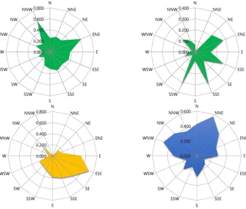
is impacted to a greater extend by local sources (see additional discussion below). CPF plots shows that the top 25 % TGM concentrations were associated with winds from the NNW and eastern direction, pointing towards northeastern China and inland Korean sources; however, when the criterion was set to the top 10 % regional transport from China became less important and the sources located in southern and eastern

20

areas of Korea were identified as important source areas (Fig. 5). The CPF plot for GOM is significantly different from the one for PBM. High PBM concentrations were as-sociated with northern winds while GOM concentrations were enhanced during south-eastern winds.

These results suggest that for PBM regional transport from Chinese and North Korea

25

(13)

ACPD

15, 32931–32966, 2015

concentrations

G.-S. Lee et al.

Title Page

Tables Figures

◭ ◮

Back Close

Full Screen / Esc

Discussion

P

a

per

|

Discussion

P

a

per

|

Discussion

P

a

per

|

Discussion

P

a

per

|

there was no relationship between GOM and SO₂concentrations. Total SO₂emissions from power plants in China (18.6 Tg yr−1) are much larger than in Korea (0.09 Tg yr−1), and SO2 emission rates per capita and per area in China also greatly surpass those

in Korea (Lu et al., 2010). Much larger SO2 emissions in China raise the background

SO₂ concentration in the region and may mask any correlation between GOM and

5

SO2 even if coal fired power plants located south of the sampling site impacted GOM

concentrations. In support of this hypothesis the pollution rose indicates that high SO2

concentrations are associated with westerly winds while high GOM concentrations are associated with southerly winds. It should be noted that only the top 25 % of GOM and PBM concentrations were used as the criteria for the CPF plot because the numbers

10

of samples for both species were significantly less than for TGM due to their longer sampling duration (12 h).

Among the eight sampling periods, the second period (April 2013) had the highest TGM, PBM and the second highest GOM average concentration, and SO₂, NO₂, CO, and PM10 were also quite high (Table 1). During this period, TGM was statistically 15

well correlated with SO2(r =0.55), NO2(r=0.56), and CO (r=0.36), with the highest

Pearson correlation coefficient with NO₂, the characteristic local pollutant. In addition, the CPF plot (for TGM) and the back-trajectories were also associated with easterly winds transporting air masses from major Korean urban areas, supporting the previous suggestion that inland sources enhanced all three Hg concentrations during the second

20

sampling period.

In contrast the fifth sampling period had the lowest GOM, PBM and the second lowest TGM concentrations (Table 1). Note however that the TGM concentrations for the first couple of days reached approximately 5 ng m−3 and gradually decreased to about 1 ng m−3during the last days of sampling (Fig. 2), indicating that there was likely

25

(14)

ACPD

15, 32931–32966, 2015

concentrations

G.-S. Lee et al.

Title Page

Tables Figures

◭ ◮

Back Close

Full Screen / Esc

Discussion

P

a

per

|

Discussion

P

a

per

|

Discussion

P

a

per

|

Discussion

P

a

per

|

the ocean boundary layer. Although Hg can be emitted from ocean surface (Han et al., 2007; UNEP, 2013) heavy rain and low solar radiation occurring during the last two days of this period probably inhibited emissions of Hg from the ocean surface.

3.2.1 GOM/PBM ratio

According to the CFP results, regional sources in China located NW and NE of the

5

sampling site were responsible for the elevated PBM concentrations while inland Ko-rean sources were important contributors to increased GOM concentrations (Fig. 5). The finding that long-range transport of TGM and PBM to the site is important is sup-ported by their significant correlation with CO (Table 3). In order to identify the relative importance of local sources relative to long-range transport, the ratio of GOM/PBM

10

was used as an indicator because the atmospheric residence time of GOM is widely regarded to be shorter than that of PBM (even though there is no consensus on what specific chemical forms are collected by KCl-coated denuders). The GOM/PBM ra-tio should be higher if local sources are more important, and the GOM/PBM ratio is likely to decrease as long-range transport becomes more important. In this study

15

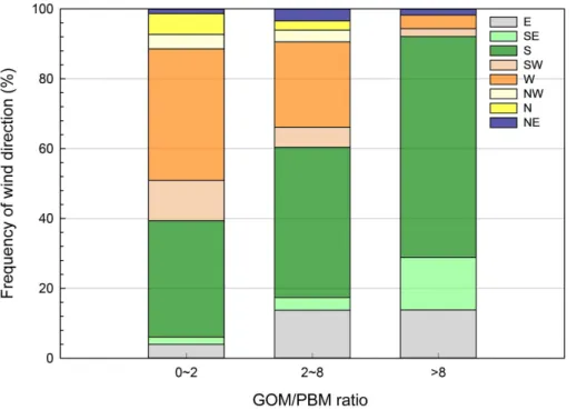
the GOM/PBM ratios were categorized into three groups: low (0–2), middle (2–8), and high (>8) and the frequency of wind direction was compared (Fig. 6). The result clearly indicates that the southerly and southeasterly winds were associated with high GOM/PBM ratios and that the westerly and northerly winds indicative of long-range transport from China prevailed at lower GOM/PBM ratios. There was a weak negative

20

correlation between the ratio of GOM/PBM and CO concentration at a significance level of 0.1 (p value=0.089), supporting the assertion that the GOM/PBM ratio de-creased with the inde-creased effect of long-range transport.

3.2.2 PSCF results

In order to locate potential source areas in more detail, PSCF was used. For TGM,

25

(15)

ACPD

15, 32931–32966, 2015

concentrations

G.-S. Lee et al.

Title Page

Tables Figures

◭ ◮

Back Close

Full Screen / Esc

Discussion

P

a

per

|

Discussion

P

a

per

|

Discussion

P

a

per

|

Discussion

P

a

per

|

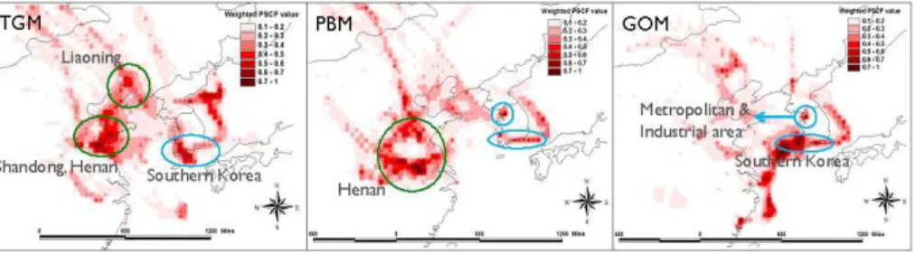
along with the southern area of Korea (Fig. 7). Liaoning province, where large non-ferrous smelters are situated, is the province with the largest Hg emission inventory in China; Shandong and Henan provinces are also large Hg emission areas, emitting about 30–40 t yr−1 (Fu et al., 2012) in part due to a large lead smelter (Wang et al., 2014), and biomass burning (Huang et al., 2011).

5

The probable source areas of PBM identified by PSCF were similar to those for TGM, indicating that both Chinese and inland Korean sources enhanced PBM con-centrations, with the exception of metropolitan (Seoul) and industrial (Incheon) areas located in northwestern South Korea which emerged as a more prominent source ar-eas for PBM than for TGM (Fig. 7). Only Korean sources including metropolitan (Seoul)

10

and the industrial areas in southern Korea were identified as probable source areas for GOM (Fig. 7); long-range transport of GOM from China was not important. The Yellow Sea between China and Korea was also associated with high PSCF values; however, it is not certain whether this is a trailing e_ffect derived by relatively short sampling duration or a real source area. A trailing effect is often observed, especially with a

lim-15

ited number of measurements or short sampling period, since PSCF evenly distributes weight along the path of trajectories so that PSCF results often identify areas upwind and downwind of real sources as a source area (Han et al., 2007). However, it should be also noted that the marine boundary layer provides good conditions for active Hg oxidation reactions due to an abundance of oxidants (Auzmendi-Murua et al., 2014);

20

therefore, the possibility of areas over the ocean being a GOM source should not be excluded.

3.2.3 Source attribution based on cluster analysis

In an e_ffort to quantify the contribution of national and foreign sources to the measured Hg concentrations the back trajectories were grouped into five clusters using the

tra-25

(16)

ACPD

15, 32931–32966, 2015

concentrations

G.-S. Lee et al.

Title Page

Tables Figures

◭ ◮

Back Close

Full Screen / Esc

Discussion

P

a

per

|

Discussion

P

a

per

|

Discussion

P

a

per

|

Discussion

P

a

per

|

2 and 3 contain trajectories from China and the Korean peninsula, but cluster 2 was more associated with Liaoning province and North Korea while cluster 3 originated more from Shandong and Henan provinces. Clusters 1 through 5 contributed 12, 25, 24, 13, and 25 % of the total time, respectively, and the associated concentrations with each cluster are shown in Table 4.

5

The TGM concentration was the highest for cluster 4; however, GOM and PBM concentrations had the lowest averages for this cluster. Cluster 4 contains the back-trajectories originating from Mongolia and Russia and passing through northeastern China before arriving at the sampling site, which suggests long-range transport was important for this cluster (Fig. 8). Average CO concentrations were pretty similar for

10

all clusters, but it was the second highest for cluster 4 (cluster 2 was highest). The highest total average GOM and PBM concentrations were associated with cluster 5 which includes trajectories distributed over the Korean peninsula, suggesting that Ko-rean sources were responsible for the enhanced GOM and PBM concentrations. For cluster 5, the highest Pearson correlation coefficient between GOM and PBM

concen-15

trations (r =0.721) was observed, indicating that both Hg species were emitted from similar sources. For other clusters, there were no statistically significant correlations between GOM and PBM except for cluster 2 (r =0.209, pvalue<0.001). In addition, both average NO2 concentration (19.4±14.9 ppb) and the correlation coefficient

be-tween NO₂ and TGM (r=0.688) were the highest for cluster 5, supporting the finding

20

of impact from Korean sources.

In order to consider both Hg concentration and the fraction of time for each cluster, the following equation was used to quantify the e_ffect of Korean and out-of- Korean sources to the Hg concentration at the receptor site.

source contribution of cluster, i =

_N

i N_total

×C_j

Pn

i=1

n _N

i N_total

×C_j

o (6)

(17)

ACPD

15, 32931–32966, 2015

concentrations

G.-S. Lee et al.

Title Page

Tables Figures

◭ ◮

Back Close

Full Screen / Esc

Discussion

P

a

per

|

Discussion

P

a

per

|

Discussion

P

a

per

|

Discussion

P

a

per

|

where (Ni/Ntotal) indicates the percentage of time associated with the cluster,i is the

number of trajectories, andC_j indicates the average Hg concentration associated with the cluster,i. Compared to the other clusters, the source contributions of clusters 1 and 4, which represent long-range transport, were relatively low for all Hg species (Table 4). Cluster 5 contributed more significantly, especially for GOM and PBM, indicating the

5

importance of Korean sources. The source contribution of cluster 2 was the highest for PBM compared to other Hg species, suggesting that North Korean sources were an important contributor to the high PBM concentrations measured, likely due to coal and biomass burning in North Korea (IEA, http://www.iea.org/stats/countryresults.asp. COUNTRY_CODE₌KP&Submit₌Submit:2012; NI, 2003).

10

In order to quantify the contribution of Korean vs. out-of-Korean sources, the source contributions of the clusters were used. Clusters 1 and 4 were used to represent the e_ffect of sources outside of Korea and the cluster 5 was used to indicate the e_ffect of sources in Korea. Since clusters 2 and 3 contain mixed trajectories from Korea and out-of-Korea their contribution was divided evenly between in and out of Korea. The results

15

indicate that the sources in Korea and outside Korea contributed about 50 % each to the TGM mass collected at the sample site during the sampling period while the Korean sources affected GOM and PBM more significantly, accounting for approximately 55 and 56 %, respectively (Table 4). These results augment the CPF and PSCF results which only use concentrations that are in the top 25th percentile. While CPF and PSCF

20

found that for high concentration events Korean sources were most important for GOM while for TGM and PBM long-range and regional transport from China and North Korea were also important, the cluster based approach suggests that for all 3 species on average approximately 50 % of the mass originates in Korea and 50 % of the mass originates outside of Korea.

(18)

ACPD

15, 32931–32966, 2015

concentrations

G.-S. Lee et al.

Title Page

Tables Figures

◭ ◮

Back Close

Full Screen / Esc

Discussion

P

a

per

|

Discussion

P

a

per

|

Discussion

P

a

per

|

Discussion

P

a

per

|

4 Conclusion and implications

This study was initiated to identify the sources affecting speciated mercury concentra-tions measured on an island located between mainland Korea and Eastern China. Vari-ous tools were used to locate and quantify the sources, including correlations with other pollutants, CPF, and the back-trajectory based analysis (PSCF and cluster analysis).

5

The results consistently show that Korean sources are most important for GOM while for other Hg species (TGM and PBM) long-range and regional transport from China and North Korea were also important. Existing methods including PSCF and CPF are able to locate the source direction and areas, but do not consider the frequency of the wind directions which can affect the long-term concentrations at the receptor site. In

10

this study, a new approach considering both the cluster frequency and the Hg con-centration associated with each cluster was used to quantify the source contribution at the sampling site. On average contributions from out-of-Korean sources were similar to Korean sources for TGM whereas Korean sources contributed approximately 55–56 % of the GOM and PBM mass compared to the out-of-Korea sources.

15

The ratio of GOM/PBM proved to be a useful tool for identifying the relative signif-icance of local sources vs. long-range transport. The GOM/PBM ratio decreased as the effect of long-range transport increased and vice versa since GOM has a shorter atmospheric residence time than PBM. The reciprocal of the PBM/GOM ratio was negatively correlated with atmospheric temperature and positively correlated with

rel-20

ative humidity, suggesting that the secondary formation of PBM through gas-particle partitioning of GOM was an important input for atmospheric PBM concentration at low temperature and high relative humidity. This result also suggests that the secondary formation of PBM becomes more important as the significance of long-range transport increased.

25

(19)

ACPD

15, 32931–32966, 2015

concentrations

G.-S. Lee et al.

Title Page

Tables Figures

◭ ◮

Back Close

Full Screen / Esc

Discussion

P

a

per

|

Discussion

P

a

per

|

Discussion

P

a

per

|

Discussion

P

a

per

|

the results, and wrote the paper. Yong S. Seo, Seung. M. Yi, and Thomas M. Holsen also interpreted the results and approved the final paper.

Acknowledgements. This work was funded by the National Research Foundation of Korea (NRF) grant funded by the Korea government (MSIP) (No. 2015R1A2A2A03008301) and the Korea Ministry of Environment (MOE) as “the Environmental Health Action Program”. This

re-5

search was also supported by 2014 Research Grant from Kangwon National University (No. C1011758-01-01).

Disclaimer.The authors declare no conflict of interest.

References

AMAP/UNEP: Technical Background Report on the Global Anthropogenic Mercury

Assess-10

ment 2013, Arctic Monitoring and Assessment Programme, Oslo, Norway/UNEP Chemicals Branch, Geneva, Switzerland, vi+263 pp., 2013.

Amos, H. M., Jacob, D. J., Holmes, C. D., Fisher, J. A., Wang, Q., Yantosca, R. M., Cor-bitt, E. S., Galarneau, E., Rutter, A. P., Gustin, M. S., Steffen, A., Schauer, J. J., Gray-don, J. A., Louis, V. L. St., Talbot, R. W., Edgerton, E. S., Zhang, Y., and Sunderland, E. M.:

15

Gas-particle partitioning of atmospheric Hg(II) and its effect on global mercury deposition, Atmos. Chem. Phys., 12, 591–603, doi:10.5194/acp-12-591-2012, 2012.

Auzmendi-Murua, I., Castillo, A., and Bozzelli, J. W.: Mercury oxidation via chlorine, bromine, and iodine under atmospheric conditions: thermochemistry and kinetics, J. Phys. Chem., 118, 2959–2975, 2014.

20

Baya, A. P. and Van Heyst, B.: Assessing the trends and effects of environmental parameters on the behaviour of mercury in the lower atmosphere over cropped land over four seasons, Atmos. Chem. Phys., 10, 8617–8628, doi:10.5194/acp-10-8617-2010, 2010.

Cheng, I., Zhang, L., Mao, H., Blanchard, P., Tordon, R., and John, D.: Seasonal and diurnal patterns of speciated atmospheric mercury at a coastal-rural and coastal-urban site, Atmos.

25

Environ., 82, 193–205, 2014.

(20)

ACPD

15, 32931–32966, 2015

concentrations

G.-S. Lee et al.

Title Page

Tables Figures

◭ ◮

Back Close

Full Screen / Esc

Discussion

P

a

per

|

Discussion

P

a

per

|

Discussion

P

a

per

|

Discussion

P

a

per

|

Draxler, R. R., Stunder, B., Rolph, G., Stein, A., and Taylor, A.: HYSPLIT Tutorial, NOAA Air Re-sour. Lab., Silver Spring, Maryland, USA, available at: http://www.arl.noaa.gov/documents/ workshop/Spring2011/HYSPLIT_Tutorial.pdf (last access: 1 February 2015), 2011.

Draxler, R. R., Stunder, B., Rolph, G., Stein, A., and Taylor, A.: HYSPLIT_4 User’s Guide, NOAA Air Resour. Lab., Silver Spring, Maryland, USA, available at: http://www.arl.noaa.gov/

5

documents/reports/hysplit_user_guide.pdf (last access: 1 February 2015), 2014.

Driscoll, C. T., Han, Y. J., Chen, C. Y., Evers, D. C., Lambert, K. F., Holsen, T. M., Kamman, N. C., and Munson, R. K.: Mercury contamination in forest and freshwater ecosystems in the North-eastern United States, Bioscience, 57, 17–28, 2007.

Edgerton, E. S.: Field investigations of RGM and fine particulate Hg measurement bias using

10

dual Tekran analyzers, in: ICMGP 2015, Jeju, Korea, 19 June 2015, 19M-S07-O-3, 2015. Fang, G. C., Zhang, L., and Huang, C. S.: Measurement of size-fractionated concentration and

bulk dry deposition of atmospheric particulate bound mercury, Atmos. Environ., 61, 371–377, 2012.

Feng, X., Lu, J. Y., Conrad, D. G., Hao, Y., Banic, C. M., and Schroeder, W. H.: Analysis of

15

inorganic mercury species associated with airborne particulate matter/aerosols: method de-velopment, Anal. Bioanal. Chem., 380, 683–689, 2004.

Finley, B. D., Jaffe, D. A., Call, K., Lyman, S., Gustin, M. S., Peterson, C., Miller, M., and Ly-man, T.: Development, testing, and deployment of an air sampling manifold for spiking ele-mental and oxidized mercury during the Reno atmospheric mercury intercomparison

experi-20

ment (RAMIX), Environ. Sci. Technol., 47, 7277–7284, 2013.

Fu, X., Feng, X., Qiu, G., Shang, L., and Zhang, H.: Speciated atmospheric mercury and its potential source in Guiyang, China, Atmos. Environ., 45, 4205–4212, 2011.

Gratz, L. E., Keeler, G. J., Marsik, F. J., Barres, J. A., and Dvonch, T.: Atmospheric transport of speciated mercury across southern Lake Michigan: influence from emission sources in the

25

Chicago/Gary urban area, Sci. Total Environ., 448, 84–95, 2013.

Gustin, M. S., Huang, J., Miller, M. B., Peterson, C., Jaffe, D. A., Ambrose, J., Finley, B. D., Lyman, S. N., Call, K., Talbot, R., Feddersen, D., Mao, H., and Lindberg, S. E.: Do we under-stand what the mercury speciation instruments are actually measuring? Results of RAMIX, Environ. Sci. Technol., 47, 7295–7306, 2013.

30

(21)

ACPD

15, 32931–32966, 2015

concentrations

G.-S. Lee et al.

Title Page

Tables Figures

◭ ◮

Back Close

Full Screen / Esc

Discussion

P

a

per

|

Discussion

P

a

per

|

Discussion

P

a

per

|

Discussion

P

a

per

|

Han, Y. J., Kim, J. E., Kim, P. R., Kim, W. J., Yi, S. M., Seo, Y. S., and Kim, S. H.: General trends of Atmospheric mercury concentrations in urban and rural areas in Korea and characteristics of high-concentration events, Atmos. Environ., 94, 754–764, 2014.

Hedgecock, I. M. and Pirrone, N.: Chasing quicksilver: modeling the atmospheric lifetime of Hg0(g) in the marine boundary layer at various latitudes, Environ. Sci. Technol., 38, 69–76,

5

2004.

Huang, J., Choi, H. D., Hopke, P. K., and Holsen, T. M.: Ambient mercury sources in Rochester, NY: results from principal components analysis (PCA) of mercury monitoring network data, Environ. Sci. Technol., 44, 8441–8445, 2010.

Huang, J., Miller, M. B., Weiss-Penzias, P., and Gustin, M. S.: Comparison of gaseous oxidized

10

Hg measured by KCl-coated denuders, and nylon and cation exchange membranes, Environ. Sci. Technol., 47, 7307–7316, 2013.

Huang, X., Li, M., Friedli, H. R., Song, Y., Chang, D., and Zhu, L.: Mercury emissions from biomass burning in China, Environ. Sci. Technol., 45, 9442–9448, 2011.

Jaffe, D. A., Lyman, S., Amos, H. M., Gustin, M. S., Huang, J., Selin, N. E., Levin, L.,

Ss-15

chure, A. T., Mason, R. P., Talbot, R., Rutter, A., Finley, B., Jaeglé, L., Shah, V., McClure, C., Ambrose, J., Gratz, L., Lindberg, S., Weiss-Penzias, P., Sheu, G. R., Fedddersen, D. D., Hor-vat, M., Dastoor, A., Hynes, A. J., Mao, H., Sonke, J. E., Slemr, F., Fisher, J. A., Ebinghaus, R., Zhang, Y., and Edwards, G.: Progress on understanding atmospheric mercury hampered by uncertain measurements, Environ. Sci. Technol., 48, 7204–7206, 2014.

20

Kim, J. H., Park, J. M., Lee, S. B., Pudasainee, D., and Seo, Y. C.: Anthropogenic mercury emission inventory with emission factors and total emission in Korea, Atmos. Environ., 44, 2714–2721, 2010.

Kim, P. R., Han, Y. J., Holsen, T. M., and Yi, S. M.: Atmospheric particulate mercury: concen-trations and size distributions, Atmos. Environ., 61, 94–102, 2012.

25

Kim, S. H., Han, Y. J., Holsen, T. M., and Yi, S. M.: Characteristics of atmospheric speciated mercury concentrtions (TGM, Hg(II), and Hg(p)) in Seoul, Korea, Atmos. Environ., 43, 3267– 3274, 2009.

Lan, X., Talbot, R., Castro, M., Perry, K., and Luke, W.: Seasonal and diurnal variations of atmospheric mercury across the US determined from AMNet monitoring data, Atmos. Chem.

30

Phys., 12, 10569–10582, doi:10.5194/acp-12-10569-2012, 2012.

(22)

ACPD

15, 32931–32966, 2015

concentrations

G.-S. Lee et al.

Title Page

Tables Figures

◭ ◮

Back Close

Full Screen / Esc

Discussion

P

a

per

|

Discussion

P

a

per

|

Discussion

P

a

per

|

Discussion

P

a

per

|

Lee, G. S., Kim, P. R., Han, Y. J., Holsen, T. M., and Lee, S. H.: Tracing sources of total gaseous mercury to Yongheung Island offthe coast of Korea, Atmosphere, 5, 273–291, 2014. Lin, C. J. and Pehkonen, S. O.: The chemistry of atmospheric mercury: a review, Atmos.

Envi-ron., 33, 2067–2079, 1999.

Liu, B., Keeler, G. J., Timothy Dvonch, J., Barres, J. A., Lynam, M. M., Marsik, F. J., and

Mor-5

gan, J. T.: Urban-rural differences in atmospheric mercury speciation, Atmos. Environ., 44, 2013–2023, 2010.

Lu, W., Zhu, Z. Y., and Liu, W. P.: Salt water intrusion numerical simulation on application based on FEFLOW, Ground Water, 32, 19–21, 2010.

Lyman, S. N. and Gustin, M. S.: Determinants of atmospheric mercury concentrations in Reno,

10

Nevada, USA, Sci. Total. Environ., 408, 431–438, 2009.

Lyman, S. N., Jaffe, D. A., and Gustin, M. S.: Release of mercury halides from KCl denuders in the presence of ozone, Atmos. Chem. Phys., 10, 8197–8204, doi:10.5194/acp-10-8197-2010, 2010.

Lynam, M. M. and Keeler, G. J.: Automated speciated mercury measurements in Michigan,

15

Environ. Sci. Technol., 39, 9253–9562, 2005.

Malcolm, E. G. and Keeler, G. J.: Evidence for a sampling artifact for particulate-phase mercury in the marine atmosphere, Atmos. Environ., 41, 3352–3359, 2007.

Mao, H., Talbot, R., Hegarty, J., and Koermer, J.: Speciated mercury at marine, coastal, and inland sites in New England – Part 2: Relationships with atmospheric physical parameters,

20

Atmos. Chem. Phys., 12, 4181–4206, doi:10.5194/acp-12-4181-2012, 2012.

Mason, R. P. and Sullivan, K. A.: Mercury in Lake Michigan, Environ. Sci. Technol., 31, 942– 947, 1997.

Mason, R. P., Morel, F. M. M., and Hemond, H. F.: The role of microorganisms in elemental mercury formation in natural water, Water Air Soil Pollut., 80, 775–787, 1995.

25

McClure, C. D., Jaffe, D. A., and Edgerton, E. S.: Evaluation of the KCl denuder method for gaseous oxidized mercury using HgBr₂at an In-Service AMNet site, Environ. Sci. Technol., 48, 11437–11444, 2014.

NI, Nautilus Institute for Security and Sustainable Development: The DPRK Energy Sector: Es-timated Year 2000 Energy Balance and Suggested Approaches to Sectoral Redevelopment,

30

Berkeley, CA, USA, 2003

(23)

ACPD

15, 32931–32966, 2015

concentrations

G.-S. Lee et al.

Title Page

Tables Figures

◭ ◮

Back Close

Full Screen / Esc

Discussion

P

a

per

|

Discussion

P

a

per

|

Discussion

P

a

per

|

Discussion

P

a

per

|

and Todd, D. E.: Mercury distribution across 14 US forests. Part I: Spatial patterns of con-centrations in biomass, litter, and soils, Environ. Sci. Technol., 45, 3974–3981, 2011. Pirrone, N., Keeler, G. J., and Nriagu, J. O.: Regional differences in worldwide emissions of

mercury to the atmosphere, Atmos. Environ., 30, 2981–2987, 1996.

Pirrone, N., Aas, W., Cinnirella, S., Ebinghaus, R., Hedgecock, I. M., Pacyna, J., Sprovieri, F.,

5

and Sunderland, E. M.: Toward the next generation of air quality monitoring: mercury, Atmos. Environ., 80, 599–611, 2013.

Polissar, A. V., Hopke, P. K., and Harris, J. M.: Source regions for atmospheric aerosol mea-sured at Barrow, Alaska, Environ. Sci. Technol., 35, 4214–4226, 2001a.

Polissar, A. V., Hopke, P. K., and Poirot, R. L.: Atmospheric aerosol over Vermont: chemical

10

composition and sources, Environ. Sci. Technol., 35, 4604–4621, 2001b.

Rutter, A. P. and Schauer, J. J.: The effect of temperature on the gas-particle partitioning of reactive mercury in atmospheric aerosols, Atmos. Environ., 41, 8647–8657, 2007.

Seinfeld, J. H. and Pandis, S. N.: Atmospherical Chemistry and Physics: from Air Pollution to Climate Change, 2nd edn., John Wiley & Sons, Inc., Hoboken, NJ, USA, 2006.

15

Subir, M., Ariya, P. A., and Dastoor, A. P.: A review of uncertainties in atmospheric modeling of mercury chemistry. I. Uncertainties in existing kinetic parameters – fundamental limitations and the importance of heterogeneous chemistry, Atmos. Environ., 45, 5664–5676, 2011. Subir, M., Ariya, P. A., and Dastoor, A. P.: A review of the sources of uncertainties in atmospheric

mercury modeling. II. Mercury surface and heterogeneous chemistry – a missing link, Atmos.

20

Environ., 46, 1–10, 2012.

Talbot, R., Mao, H., Feddersen, D., Smith, M., Kim, S. Y., Sive, B., Haase, K., Ambrose, J., Zhou, Y., and Russo, R.: Comparison of particulate mercury measured with manual and automated methods, Atmosphere, 2, 1–20, 2011.

UNEP: The global atmospheric mercury assessment, UNEP Chemicals Branch, Geneva,

25

Switzerland, 2013.

US EPA: Mercury Study Report to Congress. Office of Air Quality Planning and Standards, Research Triangle Park, NC, USA, and O_ffice of Research and Development, Washington, DC, USA, EPA-452/R-97-005, 1997.

Wan, Q., Feng, X. B., Julia, L., Zheng, W., Song, X. J., Han, S. J., and Xu, H.: Atmospheric

30

(24)

ACPD

15, 32931–32966, 2015

concentrations

G.-S. Lee et al.

Title Page

Tables Figures

◭ ◮

Back Close

Full Screen / Esc

Discussion

P

a

per

|

Discussion

P

a

per

|

Discussion

P

a

per

|

Discussion

P

a

per

|

Wan, Q., Feng, X. B., Julia, L., Zheng, W., Song, X. J., Han, S. J., and Xu, H.: Atmospheric mer-cury in Changbai Mountain area, northeastern China. II. The distribution of reactive gaseous mercury and particulate mercury and mercury deposition fluxes, Environ. Res., 109, 721– 727, 2009b.

Wang, L., Wang, S., Zhang, L., Wang, Y., Zhang, Y., Nielsen, C., McElroy, B. M., and Hao, J.:

5

Source apportionment of atmospheric mercury pollution in China using the GEOS-Chem model, Environ. Pollut., 190, 166–175, 2014.

Wang, S., Holsen, T. M., Huang, J., and Han, Y.-J.: Evaluation of various methods to measure particulate bound mercury and associated artifacts, Atmos. Chem. Phys. Discuss., 13, 8585– 8614, doi:10.5194/acpd-13-8585-2013, 2013.

10

Weiss-Penzias, P., Jaffe, D. A., Mcclintick, A., Prestbo, E. M., and Landis, M. S.: Gaseous elemental mercury in the marine boundary layer: evidence for rapid removal in anthropogenic pollution, Environ. Sci. Technol., 37, 3755–3763, 2003.

Weiss-Penzias, P., Ja_ffe, D. A., Swartzendruber, P., Dennison, J. B., Chand, D., Hafner, W., and Prestbo, E.: Observations of Asian air pollution in the free troposphere at Mount Bachelor

15

Observatory during the spring of 2004, J. Geophys. Res., 111, 1–15, 2006.

Xiu, G. L., Jin, Q. X., Zhang, D. N., Shi, S. Y., Huang, X. J., Zhang, W. Y., Bao, L., Gao, P. T., and Chen, B.: Characterization of size-fractionated particulate mercury in Shanghai ambient air, Atmos. Environ., 39, 419–427, 2005.

Xiu, G. L., Cai, J., Zhang, W. Y., Zhang, D. N., Bueler, A., Lee, S. C., Shen, Y., Xu, L. H.,

20

Huang, X. J., and Zhang, P.: Speciated mercury in size fractionated particles in Shanghai ambient air, Atmos. Environ., 43, 3145–3154, 2009.

Xu, L. L., Chen, J. S., Yang, L. M., Niu, Z. C., Tong, L., Yin, L. Q., and Chen, Y. T.: Charac-teristics and sources of atmospheric mercury speciation in a coastal city, Xiamen, China, Chemosphere, 119, 530–539, 2015.

25

(25)

ACPD

15, 32931–32966, 2015

concentrations

G.-S. Lee et al.

Title Page

Tables Figures

◭ ◮

Back Close

Full Screen / Esc

Discussion

P

a

per

|

Discussion

P

a

per

|

Discussion

P

a

per

|

Discussion

P

a

per

|

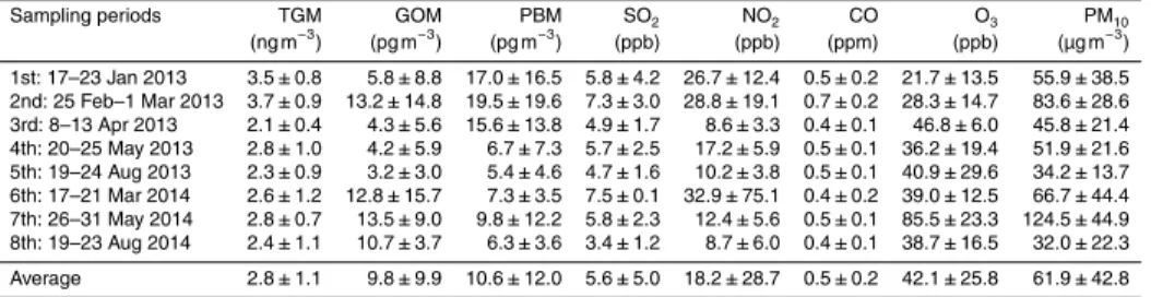
Table 1. Summarized concentrations of speciated Hg and other typical pollutants for each

sampling period.

Sampling periods TGM GOM PBM SO2 NO2 CO O3 PM10

(ng m−3₎ _{(pg m}−3₎ _{(pg m}−3₎ _(ppb) _(ppb) _(ppm) _(ppb) _{(µg m}−3₎

(26)

ACPD

15, 32931–32966, 2015

concentrations

G.-S. Lee et al.

Title Page

Tables Figures

◭ ◮

Back Close

Full Screen / Esc

Discussion

P

a

per

|

Discussion

P

a

per

|

Discussion

P

a

per

|

Discussion

P

a

per

|

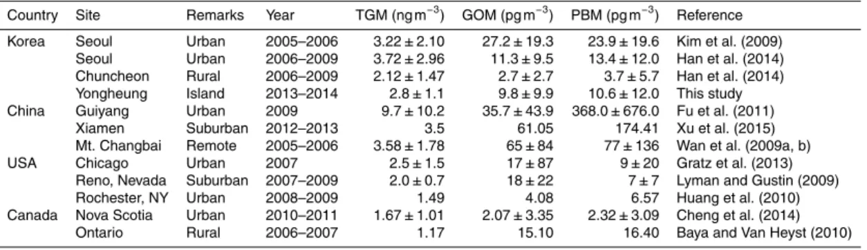
Table 2.Comparisons of measured Hg concentrations with those reported in other studies.

Country Site Remarks Year TGM (ng m−3

) GOM (pg m−3

) PBM (pg m−3

) Reference Korea Seoul Urban 2005–2006 3.22±2.10 27.2±19.3 23.9±19.6 Kim et al. (2009)

Seoul Urban 2006–2009 3.72±2.96 11.3±9.5 13.4±12.0 Han et al. (2014) Chuncheon Rural 2006–2009 2.12±1.47 2.7±2.7 3.7±5.7 Han et al. (2014) Yongheung Island 2013–2014 2.8±1.1 9.8±9.9 10.6±12.0 This study China Guiyang Urban 2009 9.7±10.2 35.7±43.9 368.0±676.0 Fu et al. (2011)

Xiamen Suburban 2012–2013 3.5 61.05 174.41 Xu et al. (2015) Mt. Changbai Remote 2005–2006 3.58±1.78 65±84 77±136 Wan et al. (2009a, b) USA Chicago Urban 2007 2.5±1.5 17±87 9±20 Gratz et al. (2013)

Reno, Nevada Suburban 2007–2009 2.0±0.7 18±22 7±7 Lyman and Gustin (2009) Rochester, NY Urban 2008–2009 1.49 4.08 6.57 Huang et al. (2010) Canada Nova Scotia Urban 2010–2011 1.67±1.01 2.07±3.35 2.32±3.09 Cheng et al. (2014)

(27)

ACPD

15, 32931–32966, 2015

concentrations

G.-S. Lee et al.

Title Page

Tables Figures

◭ ◮

Back Close

Full Screen / Esc

Discussion

P

a

per

|

Discussion

P

a

per

|

Discussion

P

a

per

|

Discussion

P

a

per

|

Table 3.Correlation coe_fficients andpvalues (in parenthesis) for speciated Hg with other

pol-lutants for the whole sampling period. Correlation coefficients with an asterisk indicate a statis-tically significant relationship atα=0.05.

TGM GOM SO2 NO2 CO O3 PM10

(28)

ACPD

15, 32931–32966, 2015

concentrations

G.-S. Lee et al.

Title Page

Tables Figures

◭ ◮

Back Close

Full Screen / Esc

Discussion

P

a

per

|

Discussion

P

a

per

|

Discussion

P

a

per

|

Discussion

P

a

per

|

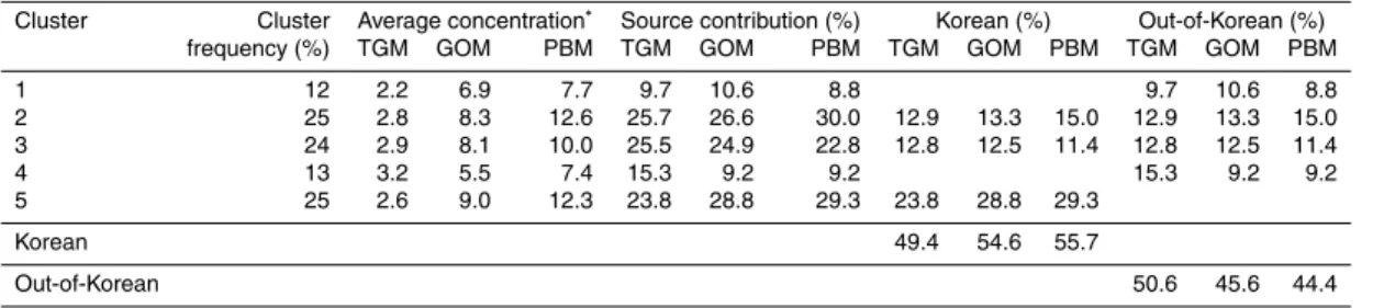
Table 4.Estimated contribution of Korean and out-of-Korean sources on variations of speciated

Hg concentration.

Cluster Cluster Average concentration∗

Source contribution (%) Korean (%) Out-of-Korean (%) frequency (%) TGM GOM PBM TGM GOM PBM TGM GOM PBM TGM GOM PBM

1 12 2.2 6.9 7.7 9.7 10.6 8.8 9.7 10.6 8.8

2 25 2.8 8.3 12.6 25.7 26.6 30.0 12.9 13.3 15.0 12.9 13.3 15.0 3 24 2.9 8.1 10.0 25.5 24.9 22.8 12.8 12.5 11.4 12.8 12.5 11.4

4 13 3.2 5.5 7.4 15.3 9.2 9.2 15.3 9.2 9.2

5 25 2.6 9.0 12.3 23.8 28.8 29.3 23.8 28.8 29.3

Korean 49.4 54.6 55.7

Out-of-Korean 50.6 45.6 44.4

∗

TGM is shown in ng m−3

while for both GOM and PBM the units are pg m−3

(29)

ACPD

15, 32931–32966, 2015

concentrations

G.-S. Lee et al.

Title Page

Tables Figures

◭ ◮

Back Close

Full Screen / Esc

Discussion

P

a

per

|

Discussion

P

a

per

|

Discussion

P

a

per

|

Discussion

P

a

per

|

Figure 1. (a)The sampling site in Yongheung Island (the star mark).(b)Anthropogenic mercury

(30)

ACPD

15, 32931–32966, 2015

concentrations

G.-S. Lee et al.

Title Page

Tables Figures

◭ ◮

Back Close

Full Screen / Esc

Discussion

P

a

per

|

Discussion

P

a

per

|

Discussion

P

a

per

|

Discussion

P

a

per

|

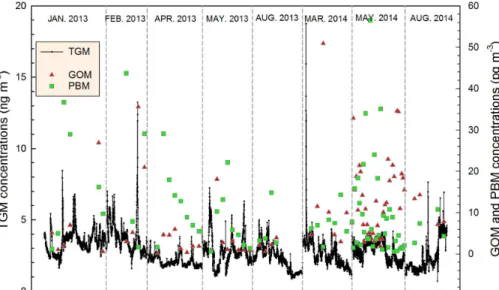
Figure 2.TGM, GOM, and PBM concentrations measured during the eight sampling periods.

(31)

ACPD

15, 32931–32966, 2015

concentrations

G.-S. Lee et al.

Title Page

Tables Figures

◭ ◮

Back Close

Full Screen / Esc

Discussion

P

a

per

|

Discussion

P

a

per

|

Discussion

P

a

per

|

Discussion

P

a

per

|

Figure 3.Seasonally averaged concentrations of TGM, GOM, and PBM shown as a

(32)

ACPD

15, 32931–32966, 2015

concentrations

G.-S. Lee et al.

Title Page

Tables Figures

◭ ◮

Back Close

Full Screen / Esc

Discussion

P

a

per

|

Discussion

P

a

per

|

Discussion

P

a

per

|

Discussion

P

a

per

|

Figure 4.The ratio of PBM/GOM related to atmospheric temperature and relative humidity

(33)

ACPD

15, 32931–32966, 2015

concentrations

G.-S. Lee et al.

Title Page

Tables Figures

◭ ◮

Back Close

Full Screen / Esc

Discussion

P

a

per

|

Discussion

P

a

per

|

Discussion

P

a

per

|

Discussion

P

a

per

|

Figure 5.CPF plots for TGM using the top 25 % (left upper panel) and the top 10 % (right upper