www.atmos-meas-tech.net/9/5955/2016/ doi:10.5194/amt-9-5955-2016
© Author(s) 2016. CC Attribution 3.0 License.
High-resolution observations of small-scale gravity waves
and turbulence features in the OH airglow layer
René Sedlak1, Patrick Hannawald2, Carsten Schmidt1, Sabine Wüst1, and Michael Bittner1,2
1German Remote Sensing Data Center, German Aerospace Center, Oberpfaffenhofen, Germany 2Institute of Physics, University of Augsburg, Augsburg, Germany
Correspondence to:René Sedlak ([email protected])
Received: 8 September 2016 – Published in Atmos. Meas. Tech. Discuss.: 12 September 2016 Revised: 9 November 2016 – Accepted: 25 November 2016 – Published: 12 December 2016
Abstract.A new version of the Fast Airglow Imager (FAIM) for the detection of atmospheric waves in the OH airglow layer has been set up at the German Remote Sensing Data Center (DFD) of the German Aerospace Center (DLR) at Oberpfaffenhofen (48.09◦N, 11.28◦E), Germany. The
spa-tial resolution of the instrument is 17 m pixel−1in zenith
di-rection with a field of view (FOV) of 11.1 km×9.0 km at
the OH layer height of ca. 87 km. Since November 2015, the system has been in operation in two different setups (zenith angles 46 and 0◦) with a temporal resolution of 2.5 to 2.8 s.
In a first case study we present observations of two small wave-like features that might be attributed to gravity wave instabilities. In order to spectrally analyse harmonic struc-tures even on small spatial scales down to 550 m horizontal wavelength, we made use of the maximum entropy method (MEM) since this method exhibits an excellent wavelength resolution. MEM further allows analysing relatively short data series, which considerably helps to reduce problems such as stationarity of the underlying data series from a sta-tistical point of view. We present an observation of the subse-quent decay of well-organized wave fronts into eddies, which we tentatively interpret in terms of an indication for the onset of turbulence.
Another remarkable event which demonstrates the techni-cal capabilities of the instrument was observed during the night of 4–5 April 2016. It reveals the disintegration of a rather homogenous brightness variation into several fil-aments moving in different directions and with different speeds. It resembles the formation of a vortex with a horizon-tal axis of rotation likely related to a vertical wind shear. This case shows a notable similarity to what is expected from the-oretical modelling of Kelvin–Helmholtz instabilities (KHIs).
The comparatively high spatial resolution of the presented new version of the FAIM provides new insights into the structure of atmospheric wave instability and turbulent pro-cesses. Infrared imaging of wave dynamics on the sub-kilometre scale in the airglow layer supports the findings of theoretical simulations and modellings.
1 Introduction
The reaction of hydrogen and ozone produces molecular oxygen and vibrational–rotationally excited hydroxyl (OH)∗.
OH∗ relaxes by emitting electromagnetic radiation,
espe-cially in the SWIR (shortwave infrared, commonly defined from 0.9 to 1.7 µm) range (Bates and Nicolet, 1950). The hy-droxyl forms a Chapman layer at the upper mesosphere and lower thermosphere and is the brightest component of the airglow phenomenon. The peak concentration of OH∗is
lo-cated at an altitude of ca. 87 km with a half-width of about 8 km (Baker and Stair, 1988). The OH∗mean emission
Energy and momentum transported by atmospheric waves are released into the surrounding atmosphere when insta-bilities lead to turbulence. Atmospheric instability can ei-ther be of dynamical or of convective nature. Dynamical in-stabilities are caused by wind shear, leading to formation of Kelvin–Helmholtz instabilities (KHIs; Browning, 1971), whereas convective instabilities are induced when the tem-perature lapse rate gets superadiabatic (Fritts and Alexander, 2003).
Turbulent processes are characterized to cover several magnitudes of the length scale. The complete range of tur-bulence can be divided into three parts: within the largest regime, the so-called buoyancy subrange, energy is still car-ried by waves and the buoyancy force is dominating viscos-ity. Distortions on scales below the buoyancy subrange let the transported energy cascade to smaller and even smaller structures (inertial subrange) where energy is still conserved within the eddies until it is dissipated into the atmosphere due to viscous damping (viscous subrange) (e.g. Lübken et al., 1987). It must be noted that the scale limits between the three subranges are strongly dependent on the altitude. Within the abovementioned region of the OH∗peak concentration at an
altitude of about 87 km, the inertial subrange of turbulence is on a scale of a few hundreds of metres, starting just below 1 km and reaches the viscous subrange at about 30 m (Hock-ing, 1985).
In order to deduce horizontal information of atmospheric waves, infrared camera systems have come up as a highly promising remote sensing technique (see e.g. Peterson and Kieffaber, 1973; Herse et al., 1989; Moreels et al., 2008) as they allow obtaining images of atmospheric waves. Gravity wave activity at airglow altitude of the entire night sky can be imaged using all-sky lenses (Taylor et al., 1997; Smith et al., 2009, and many others). Another application for air-glow imagers is the investigation of small-scale gravity wave structures, such as acoustic-gravity waves (e.g. Nakamura et al., 1999) or instability features (Hecht et al., 2014). A high spatio-temporal resolution is required for this purpose, which is achieved at the expense of the aperture angles of the imager. However, theoretical calculations especially in the spatial regime below 1 km are hardly supported by experi-mental observations yet, since a better spatial resolution than 500 m pixel−1is needed to image structures on these scales
(Hecht et al., 2014).
vations within the international Network for the Detection of Mesospheric Chance (NDMC, http://wdc.dlr.de/ndmc). A third system of this kind, FAIM 2, is installed for aircraft based observations on the DLR research aircraft FALCON.
In order to investigate even smaller-scale gravity wave sig-natures and turbulent features at mesopause heights, a further developed FAIM system, FAIM 3, is presented in this paper. Compared to earlier airglow imagers (Hecht et al., 1997; Ya-mada et al., 2001) the resolution has been improved by at least 1 order of magnitude in both space and time. Achieving a spatial resolution of 30 m pixel−1(zenith angle of 46◦) and
17 m pixel−1(zenith angle of 0◦) the entire inertial subrange
as well as the beginning viscous subrange of turbulence at airglow altitude is accessible to this instrument. Additionally, the temporal resolution of no longer than 2.8 s allows inves-tigating the development of transient processes like breaking wave fronts.
2 Instrumentation
FAIM 3 is the second version of the Fast Airglow Imagers established at DLR (Hannawald et al., 2016). It is based on the SWIR camera CHEETAH CL developed by Xenics nv. Its 640×512 pixel InGaAs sensor array with a pixel size
of 20 µm×20 µm is sensitive to the spectral range from 0.9
to 1.7 µm. The raw signal is converted into a 14 bit digital stream, which is sent to a frame grabber via CameraLink. The sensor is thermoelectrically cooled down to an operational temperature of 233 K. The dissipated heat is carried away by a closed circuit water cooling system. A schematic diagram of the entire setup is shown in Fig. 1.
All measurements presented here are performed at DLR at Oberpfaffenhofen (48.09◦N, 11.28◦E), southern Germany.
A 100 mm SWIR lens by Edmund Optics®is used. Its aper-ture angles have been determined to be 7.3◦in horizontal
di-rection and 5.9◦ in vertical direction. In the first
measure-ment configuration the camera was mounted on a fixed stage with a zenith angle of 46◦. The geometry of this arrangement
Figure 1.Schematic drawing of the FAIM 3 setup. The measure-ment configuration with a zenith angle of 46◦is shown here.
overall area of about 299 km2is observed with a mean spatial resolution of 30 m pixel−1. The camera is adjusted to an
az-imuth angle of 214◦. In order to record a sufficiently strong
airglow signal the integration time of the camera is set to 2.5 s. The instrument in this configuration has been in opera-tion from 18 to 30 November 2015. The data of the first case study were measured with this configuration.
In a second measurement configuration the FAIM 3 zenith angle is adjusted to 0◦. Still using the 100 mm lens, a
11.1 km×9.0 km rectangular area (100 km2) of the airglow
layer is acquired. This leads to a mean spatial resolution of 17 m pixel−1. The integration time has to be raised to 2.8 s
since the airglow intensity decreases with decreasing zenith angle due to the van Rhijn effect (van Rhijn, 1921).
A flat field correction is applied in order to remove the fixed pattern noise and the vignetting of the acquired images. In order to better judge on the overall dynamical situa-tion we operated the FAIM 3 zenith measurements simul-taneously with the FAIM 4 instrument where FAIM 4 was allowed to sense the overall sky. The temporal resolution of FAIM 4 in this case was 1.5 s while the spatial resolution is roughly 400 m pixel−1within the image centre.
3 Data analysis
The horizontal wavelengths of gravity waves in an image can be estimated by analysing the data series of the pixel inten-sities along a cross section perpendicular to the wave fronts. The distortion resulting from the abovementioned trapezium-shaped FOV projected onto rectangular images has to be cor-rected prior to analysis so that an equidistant metric scale is provided. The images are mirrored and rotated into the proper azimuthal direction so that they can be rendered true to scale onto a map (see Fig. 2). This correction is per-formed using the same algorithm as described in Hannawald et al. (2016). As a typical example, Fig. 2a–f show a se-quence of such images taken on 18 November 2015, between 22:59:55 and 23:04:11 UTC.
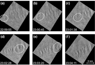
Figure 2.Image series of the case study of 18 November 2015 be-tween 22:59:55 and 23:04:11 UTC. Difference images have been chosen for presentation purposes. The images are aligned to the north. The 1.7 km wave structure extends from the western to the eastern corner with several crests being arranged in a narrow cor-ridor. The 550 m wave packet is framed in a white ellipse (a–e). One may perceive the beginning decay at 23:03:20 UTC. The entire sequence is shown in Video 1 of the Supplement. The black line, which is shown in(b), indicates the cross section along which the spectral analysis is performed in Figs. 3 and 4.
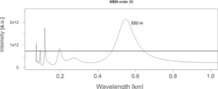
The periodic brightness variation related to a wavelike structure appears in the series of pixel intensities along a direction perpendicular to the wave fronts in the image, as shown in Fig. 3. Spectral analysis of the data series allows deducing the horizontal wavelengths. Since in our case the observed gravity waves are localized within a comparatively small area of the FOV and exhibit wavelengths of relatively small scales, the data series of pixel intensities extend over less than a hundred data points. Considering also the pro-nounced noise level, the maximum entropy method (MEM) turned out to be a powerful technique to estimate the spectral density of the data sets (Ulrych and Bishop, 1975), even if the data series is so short. As an example, Fig. 4 shows the MEM spectrum of the data series shown in Fig. 3.
lar to the wavefronts (its position is indicated by the black line in Fig. 2b) in the image of 18 November 2015, 23:00:42 UTC. The pixel range has been converted into kilometres. The orange line shows an ideal 550 m wave (fitted by hand). Only the first half of the data series shows this signal, too.
the right orderN of the underlying AR process. If the order is chosen too small several frequency peaks may not be re-solved, whereas an overestimated order will lead to further splitting of the peaks into spurious subpeaks due to noise ap-proximation (e.g. Wüst and Bittner, 2006).
4 Results
During the night from 18 to 19 November 2015 observa-tions were performed at a zenith angle of 46◦, leading to
a spatial resolution of approximately 30 m pixel−1. In order
to demonstrate the performance of the instrument, one in-teresting gravity wave event, registered between 22:59:25 and 23:04:33 UTC, is presented. The interval is shown in parts by a series of six images in Fig. 2a–f and in its en-tirety in Video 1 in the Supplement. First-order difference images (meaning the temporal derivation of the original sig-nal, here 1t=7.5 s) are shown here to help better visual-ize wave structures. The difference of two images acts as a high-pass filter, suppressing long-period oscillations and highlighting the regions with varying intensity between the two images. However, the original data are used, of course, for spectral analysis in order to retrieve the correct spatial content. It is interesting to note that a smaller-scale wave packet is propagating from the left corner of the FOV (west) to the right corner (east), apparently advected by the back-ground wind. The packet, which is marked by white circles in Fig. 2a–e, moves in the same direction as a second, larger wave structure but its wave fronts are tilted against each other horizontally by an angle of about 45◦. The larger wave
struc-ture extends nearly over the entire image from the lower left to the upper right corner of Fig. 2a–f, and the quite limited horizontal width of the wave fronts makes the wave appear to be trapped in a narrow corridor in the airglow layer. Having nearly completely passed through the FOV the wave packet seems to decompose into some disordered features as time
icance. The peak of the 550 m wave packet is clearly recognizable.
Figure 5.MEM spectra of the order of 36 of pixel intensities along the abovementioned cross section (its position is indicated by the black line in Fig. 2b) in every image taken between 23:00:17 and 23:00:55 UTC. The signature of the 550 m wave packet is found by the MEM nearly the entire period.
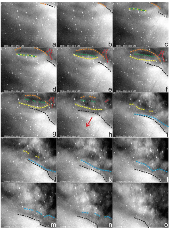
Another interesting event was observed during the night from 4 to 5 April 2016. The images (see Fig. 6a–o) have been acquired at the zenith position with a spatial resolution of about 17 m pixel−1. The dimensions of each image are
ap-proximately 11.1 km×9.0 km. The zenith images show the
sky as seen from the ground looking upwards. The upper image side corresponds to an azimuthal direction of 303◦.
Video 2 in the Supplement shows the entire event.
A wave front, indicated by the dashed black line in the images of Fig. 6, enters the FOV in the upper right corner. While it continues propagating to the lower left, a filament separates from it on the left side (Fig. 6a–b, orange). This filament moves more slowly than the wave front. At around 03:18:30 UTC (Fig. 6c) a second filament structure becomes visible below the first filament. In the further course of the image series (Fig. 6e–f) it turns out to separate into two struc-tures, a filament moving downward (yellow) and a stationary filament (green). At about 03:19:26 UTC (Fig. 6g) the orange and the green structure begin to dissolve. The yellow struc-ture continues propagating for a few more seconds and fi-nally also starts decomposing at 03:19:54 UTC (Fig. 6i). At 03:18:44 UTC (Fig. 6d) two more filaments form at the up-per right of the FOV right behind the initial wave front and are, in contrast to the other filaments, aligned perpendicular to it. They decompose at 03:19:26 UTC (Fig. 6g). While the dynamics of the filaments take their course and form a vor-tex, rotating around a horizontally oriented axis, the initial wave front (black) overtakes the other structures, retaining its original direction (indicated by the red arrow in Fig. 6h). At about 03:19:54 UTC (Fig. 6i) another filament (blue) sep-arates from it. This new filament remains stationary and starts decaying at 03:20:50 UTC (Fig. 6m). The wave front (black) keeps on propagating and leaves the FOV toward the lower left.
To put the observations into a larger spatial context, the FAIM 3 data are compared to simultaneous all-sky measure-ments taken by the FAIM 4 instrument. Since the two cam-eras are deployed next to each other, the FOV of FAIM 3 is embedded in the centre of the FOV of FAIM 4. The FAIM 4 measurements are presented in Video 3 in the Supplement. Besides the normal image, the difference image (time dif-ference of 60 s) is displayed on the right side; both images are rotated northward. The approximate FOV of FAIM 3 is indicated by the white boxes in Video 3 in the Supplement.
Figure 7. FAIM 4 all-sky image taken on 5 April 2016 at 03:20:20 UTC(a)and the magnified (zoom factor of 4) image cen-tre(b). The entire sequence is shown in Video 3 in the Supplement. Due to their spatial structure and their wavelength, we interpret the patchy structures in the starry sky as gravity wave fronts in the air-glow layer. Comparison with the respective FAIM 3 image, which has been placed at its correct position in the middle of the all-sky image, shows how the small-scale details of the wave crest can be resolved with the new instrument. The direction of propagation is indicated by the red arrow and matches with the observations of FAIM 3.
The all-sky images reveal a clear and starry sky with high gravity wave activity, which can be determined on the basis of the characteristic patchy structures. The remarkable struc-ture observed by FAIM 3 can be found again in Video 3 in the Supplement as a bright feature within the white box, propa-gating to eastern direction, which agrees with the FAIM 3 observations. Figure 7 shows the FAIM 4 all-sky image at 03:20:20 UTC with the respective FAIM 3 image embedded into it (Fig. 7a) as well as the image centre magnified by a factor of 4 (Fig. 7b).
5 Discussion
The first of the two case studies presented here shows a wave packet with a horizontal wavelength of about 550 m mov-ing in the same direction as a 1.7 km wave with the wave fronts being tilted about 45◦against the other structure. We
propagation direction is unusual (ratio approximately 1 : 6). Obviously, it cannot be described as a plane wave (of infi-nite extent). It may rather be trapped in a duct, or the entire pattern, which appears to be a wave structure, may indeed be an instability feature itself, which is not unlikely given the small dimension with an apparent wavelength of 1.7 km. It may be consequently speculated that the 1.7 km wave itself is a possible instability feature of a larger-scale wave with a horizontal wavelength of several kilometres and decays into the 550 m wave packet as a subordinate instability structure. Such dynamics have already been observed on larger scales in Hecht et al. (2014). Assuming the same scenario here, the ratio of primary to secondary wavelength is about 3.1. This number agrees quite well with earlier KHI models (Klaassen and Peltier, 1991).
While dynamical instability manifests as subordinate wave structures parallel to the initial wave fronts, convective insta-bility emerges as wave structures perpendicular to the initial gravity wave (Andreassen et al., 1994; Fritts et al., 1994). Taylor and Hapgood (1990) assume ripples to be the sig-nature of KHIs, thus being related to dynamical instability. However, past observations do not agree about this issue. While Yamada et al. (2001) have presented images of insta-bility features aligned parallel to a breaking gravity wave, Hecht et al. (1997) have observed ripple structures that were aligned perpendicular to an initial wave, which rather assigns those ripples to be caused by convective instability. In our ob-servations none of both cases is favoured as the wave fronts of the 550 m wave packet are aligned by an angle of 45◦to
the superordinate 1.7 km wave. This supports the assump-tion of Hecht (2004) that some ripples may be generated by the combination of dynamical and convective instability. Ac-cording to Fritts et al. (1996) an initially convectively driven instability structure can be rotated by the background wind shear. This could be a possible explanation for the tilt of the wave fronts.
At around 23:03:30 UTC the 550 m wave packet starts to collapse into some disordered features, which we tentatively assign to turbulence. Following the considerations of Hock-ing (1985), observations on that scale are already situated in the inertial subrange at airglow altitudes. Similar turbulent-looking features resulting of atmospheric instabilities have been found in the measurements of Hecht et al. (2014) in the buoyancy regime. Related direct numerical simulations (DNSs) (see Fritts et al., 2014) to that data have already predicted secondary instability features below 1 km, which had not been able to observe with an airglow imager so far. However, it must be stressed that these interpretations re-main speculative at this stage as the focus of this paper is to demonstrate the capability of the FAIM 3 instrument to resolve smaller-scale dynamics in the mesopause altitude re-gion. Alternatively, the periodic structures could simply be remarkably small-scale gravity waves with wavelengths of 1.7 km and 550 m as well, without being results of atmo-spheric instability.
The second interesting event detected by FAIM 3 is a wave front, which partly separates into filament-like features while propagating through the FOV. Most of the filaments emerge parallel to the incident wave front and develop dif-ferent velocities so that the impression of a horizontally ro-tating vortex arises. This can likely be assigned to instabil-ity driven by wind shear, i.e. KHIs. The filament structures decay into disorganized features, which resemble the tur-bulent collapse of the wave packet on 18 November 2015. On larger scales, other airglow observations exhibit similar-looking breakdown events of gravity wave fronts, like in Hecht et al. (2014). The effects of KHI dynamics in the air-glow layer have been modelled using DNSs and large eddy simulations (Fritts et al., 2014). The vortex structure as well as the filament features turns out to be a typical manifesta-tion of turbulence due to KHIs. However, in our observamanifesta-tions also some filaments aligned perpendicular to the initial wave front have been formed (Fig. 6d–g, red). These indicate the presence of convective instability. The high gravity wave ac-tivity of the overall night sky, revealed by FAIM 4 all-sky measurements at the same time, certainly contributes to at-mospheric instability by influencing the lapse rate. Thus it could be again the combination of dynamical and convective instability which triggers the event on 5 April 2016.
The aforementioned wave front is also visible in the all-sky images, but a close inspection of Video 3 in the Supple-ment hardly allows perceiving indications for the separation of parts from the bright crest. Zooming into the all-sky image (Fig. 7b) shows that only the high-resolution measurements of FAIM 3 can reveal closer details of this structure.
6 Summary and conclusions
In order to observe smaller-scale gravity wave events and instabilities or turbulence features in the metre regime, the established airglow imaging system FAIM (Hannawald et al., 2016) has been improved with regard to spatial reso-lution, using an InGaAs sensor array with the 4-fold num-ber of pixels (327 680) and a 100 mm SWIR lens manu-factured by Edmund Optics®. The mean spatial resolution of 200 m pixel−1 at a 45◦ zenith angle and 120 m pixel−1
at zenith position achieved by the established FAIM system has been increased to 30 and 17 m pixel−1respectively.
Mea-surements have been taken at Oberpfaffenhofen (48.09◦N,
11.28◦E), southern Germany, at a zenith angle of 46◦and an
azimuth angle of 214◦as well as in zenith position.
Two case studies are presented. On 18 November 2015 from 22:59:25 to 23:04:33 UTC a wavelike structure with a wavelength of 1.7 km and a smaller feature with a wave-length of 550 m propagate in the same direction. Their wave fronts are tilted against each other by an angle of approxi-mately 45◦. The 1.7 km wave is estimated as having a
gest that the event of 18 November 2015 could be triggered by KHIs.
Zenith measurements on 5 April 2016 from 03:15:58 to 03:27:46 UTC exhibit the breakdown of a wave front into a vortex structure and the subsequent decay into disorganized features, probably due to turbulence. Characteristic dynam-ics of filament-like features indicate that instability could be generated by wind shear. The observations look similar to modellings of KHI development and the consecutive turbu-lence dynamics of waves in the airglow layer (Fritts et al., 2014). Comparisons with parallel measurements of FAIM 4 obtaining all-sky images reveal the high gravity wave activ-ity all over the sky at that time, which might have contributed to increased atmospheric instability.
It has been demonstrated that FAIM 3 is able to image the dynamics of gravity waves on scales significantly be-low 1 km. FAIM 3 not only resolves the entire inertial range; it also provides insight into the beginning viscous sub-range of turbulence. As concerns airglow imaging this opens a new scale range of dynamic processes that can be moni-tored, like shown in the first case study. Whereas structures like the larger one (periodicity∼1.7 km) can now be studied
in greater detail with FAIM 3, structures like the smaller one (550 m) are now observable for the first time at all.
Concerning the connection of our observations with pre-vious work in terms of scientific aspects, the second event is more evident. It shows the formation and temporal evolution of an instability feature. Due to the high temporal resolution (2.8 s) one can determine the initial formation of this struc-ture and its later orientation relative to the initial wave field. Thus, observations of this kind are valuable for determining the nature of instability concerning the question of whether such features are primarily driven convectively or dynami-cally.
In this context several previous studies (e.g. Yamada et al., 2001; Hecht et al., 2004; Fritts et al., 1996) question of whether “ripples” were initially formed parallel or perpen-dicular to the gravity wave fronts and then rotated by the local wind fields or formed as a combination of both insta-bilities. These possibilities severely complicate scientific in-terpretation of ripple occurrence. With the new observation capabilities provided by the FAIM 3 we can now study this initial formation in greater detail. The two instability events presented in this paper appear to be driven dynamically, but
since it provides the opportunity to more closely investigate specific airglow structures with a much higher spatial resolu-tion, as demonstrated in the second case study in this paper.
Operational zenith measurements with a mean spatial resolution of 17 m pixel−1 and a temporal resolution of
2.8 s have been performed automatically every night since 22 February 2016 at Oberpfaffenhofen, Germany.
7 Data availability
The data are archived at the WDC-RSAT (World Data Cen-ter for Remote Sensing of the Atmosphere, http://wdc.dlr.de). FAIM 3 is part of the Network for the Detection of Meso-spheric Change, NDMC (http://wdc.dlr.de/ndmc).
The Supplement related to this article is available online at doi:10.5194/amt-9-5955-2016-supplement.
Acknowledgements. Parts of this research received funding from the Bavarian State Ministry of the Environment and Consumer Protection by grant number TUS01UFS-67093.
The article processing charges for this open-access publication were covered by a Research
Centre of the Helmholtz Association.
Edited by: L. Hoffmann
Reviewed by: two anonymous referees
References
Adams, G. W., Peterson, A. W., Brosnahan, J. W., and Neuschaefer, J. W.: Radar and optical observations of mesospheric wave activ-ity during the lunar eclipse of 6 July 1982, J. Atmos. Terr. Phys., 50, 11–20, 1988.
Baker, D. J. and Stair, A. T.: Rocket Measurements of the Altitude Distributions of the Hydroxyl Airglow, Phys. Scripta, 37, 611– 622, 1988.
Bates, D. R. and Nicolet, M.: Atmospheric Hydrogen, Publ. Astron. Soc. Pac., 62, 106–110, 1950.
Bittner, M., Offermann, D., Bugaeva, I. V., Kokin, G. A., Koshelkov, J. P., Krivolutsky, A., Tarasenko, D. A., Gil-Ojeda, M., Hauchecorne, A., Lübken, F.-J., de la Morena, B. A., Mourier, A., Nakane, H., Oyama, K. I., Schmidlin, F. J., Soule, I., Thomas, L., and Tsuda, T.: Long period/large scale oscilla-tions of temperature during the DYANA campaign, J. Atmos. Terr. Phys., 56, 1675–1700, 1994.
Browning, K. A.: Structure of the atmosphere in the vicinity of large-amplitude Kelvin–Helmholtz billows, Q. J. Roy. Meteor. Soc., 97, 283–299, 1971.
Fritts, D. C. and Alexander, M. J.: Gravity wave dynamics and effects in the middle atmosphere, Rev. Geophys., 41, 1003, doi:10.1029/2001RG000106, 2003.
Fritts, D. C., Isler, J. R., and Andreassen, Ø.: Gravity wave breaking in two and three dimensions 2. Three-dimensional evolution and instability structure, J. Geophys. Res., 99, 8109–8123, 1994. Fritts, D. C., Garten, J. F., and Andreassen, Ø.: Wave breaking and
transition to turbulence in stratified shear flows, J. Atmos. Sci., 53, 1057–1085, 1996.
Fritts, D. C., Wan, K., Werne, J., Lund, T., and Hecht, J. H.: Mod-eling the implications of Kelvin–Helmholtz instabilty dynamics for airglow observations, J. Geophys. Res.-Atmos., 119, 8858– 8871, doi:10.1002/2014JD021737, 2014.
Gardner, C. S., Zhao, Y., and Liu, A. Z.: Atmospheric stability and gravity wave dissipation in the mesopause region, J. Atmos. Sol.-Terr. Phy., 64, 923–929, 2002.
Hannawald, P., Schmidt, C., Wüst, S., and Bittner, M.: A fast SWIR imager for observations of transient features in OH airglow, At-mos. Meas. Tech., 9, 1461–1472, doi:10.5194/amt-9-1461-2016, 2016.
Hecht, J. H.: Instability layers and airglow imaging, Rev. Geophys., 42, RG1001, doi:10.1029/2003RG000131, 2004.
Hecht, J. H., Walterscheid, R. L., Fritts, D. C., Isler, J. R., Senft, D. C., Gardner, C. S., and Franke, S. J.: Wave breaking signatures in OH airglow and sodium densities and temperatures 1. Airglow imaging, Na lidar, and MF radar observations, J. Geophys. Res., 102, 6655–6668, 1997.
Hecht, J. H., Wan, K., Gelinas, L. J., Fritts, D. C., Walterscheid, R. L., Rudy, R. J., Liu, A. Z., Franke, S. J., Vargas, F. A., Pautet, P. D., Taylor, M. J., and Swenson, G. R.: The life cycle of instability features measured from the Andes Lidar Observatory over Cerro Pachon on 24 March 2012, J. Geophys. Res. Atmos., 119, 8872– 8898, 2014.
Herse, M., Thuillier, G., Camman, G., Chevassut, J.-L., and Fehren-bach, M.: Ground based instrument for observing near IR night-glow inhomogeneities at zenith and throughout the sky, Appl. Optics, 28, 3944–3949, doi:10.1364/AO.28.003944, 1989. Hocking, W. K.: Measurement of turbulent energy dissipation rates
in the middle atmosphere by radar techniques: A review, Radio Sci., 20, 1403–1422, 1985.
Jaynes, E. T.: New engineering applications of information theory, Proceedings of the first symposium on engineering applications of random function theory and probability, edited by: Bogdanoff, J. L. and Kozin, F., John Wiley, New York, 1963.
Klaassen, G. P. and Peltier, W. R.: The influence of stratification on secondary instability in free shear layers, J. Fluid Mech., 227, 71–106, 1991.
Lübken, F.-J., von Zahn, U., Thrane, E. V., Blix, T., Kokin, G. A., and Pachomov, S. V.: In situ measurements of turbulent energy dissipation rates and eddy diffusion coefficients during MAP/WINE, J. Atmos. Terr. Phys., 49, 763–775, 1987. Moreels, G., Clairemidi, J., Faivre, M., Mougin-Sisini, D., Kouahla,
M. N., Meriwether, J. W., Lehmacher, G. A., Vidal, E., and Veliz, O.: Stereoscopic imaging of the hydroxyl emissive layer at low latitudes, Planet. Space Sci., 56, 1467–1479, 2008.
Nakamura, T., Higashikawa, A., Tsuda, T., and Matsuhita, Y.: Sea-sonal variations of gravity wave structures in OH airglow with a CCD imager at Shigaraki, Earth Planets Space, 51, 897–906, 1999.
Peterson, A. W.: Airglow events visible to the naked eye, Appl. Op-tics, 18, 3390–3393, doi:10.1364/AO.18.003390, 1979. Peterson, A. W. and Kieffaber, L. M.: Infrared Photography of OH
Airglow Structures, Nature, 242, 321–322, 1973.
Smith, S., Baumgardner, J., and Mendillo, M.: Evidence of meso-spheric gravity-waves generated by orographic forcing in the tro-posphere, Geophys. Res. Lett., 36, doi:10.1029/2008GL036936, 2009.
Taylor, M. J. and Hapgood, M. A.: On the origin of ripple-type wave structure in the OH nightglow emission, Planet. Space Sci., 38, 1421–1430, 1990.
Taylor, M. J., Pendleton Jr., W. R., Clark, S., Takahashi, H., Gobbi, D., and Goldberg, R. A.: Image measurements of short-period gravity waves at equatorial latitudes, J. Geogr. Res., 102, 26283– 26299, doi:10.1029/96JD03515, 1997.
Ulrych, T. J. and Bishop, T. N.: Maximum entropy spectral analysis and autoregressive decomposition, Rev. Geophys. Space Phys., 13, 183–200, 1975.
van Rhijn, P. J.: On the brightness of the sky at night and the total amount of starlight, Publications of the Astronomical Laboratory at Groningen, 31, 1–83, 1921.
von Savigny, C.: Variability of OH(3-1) emission altitude from 2003 to 2011: Long-term stability and universality of the emission rate-altitude relationship, J. Atmos. Sol.-Terr. Phy., 127, 120– 128, doi:10.1016/j.jastp.2015.02.001, 2015.
Wüst, S. and Bittner, M.: Non-linear resonant wave-wave interac-tion (triad): Case studies based on rocket data and first appli-cation to satellite data, J. Atmos. Sol.-Terr. Phy., 68, 959–976, 2006.