www.j-sens-sens-syst.net/3/1/2014/ doi:10.5194/jsss-3-1-2014
©Author(s) 2014. CC Attribution 3.0 License.
Open
Access
JSSS
Journal of Sensors and Sensor SystemsNew ferromagnetic core shapes for induction sensors
C. Coillot1, J. Moutoussamy2, M. Boda3, and P. Leroy2 1
Laboratoire Charles Coulomb, BioNanoNMRI group, University Montpellier II, Place Eugene Bataillon, 34090 Montpellier, France
2LPP/CNRS/UPMC/Ecole Polytechnique, Route de Saclay, 91128 Palaiseau, France
3SubSeaStem, 25 rue des Ondes, 12000 Rodez, France
Correspondence to:C. Coillot ([email protected])
Received: 10 August 2013 – Revised: 30 October 2013 – Accepted: 5 December 2013 – Published: 15 January 2014
Abstract. Induction sensors are used in a wide range of scientific and industrial applications. One way to improve these is rigorous modelling of the sensor combined with a low voltage and current input noise pream-plifier aiming to optimize the whole induction magnetometer. In this paper, we explore another way, which consists in the use of original ferromagnetic core shapes of induction sensors, which bring substantial improve-ments. These new configurations are the cubic, orthogonal and coiled-core induction sensors. For each of them we give modelling elements and discuss their benefits and drawbacks with respect to a given noise-equivalent magnetic induction goal. Our discussion is supported by experimental results for the cubic and orthogonal configurations, while the coiled-core configuration remains open to experimental validation. The transposition of these induction sensor configurations to other magnetic sensors (fluxgate and giant magneto-impedance) is an exciting prospect of this work.
1 Introduction
The function of induction magnetometers is to measure ex-tremely weak magnetic fields. Their field of application is very large and covers soil characterization for agriculture (Sudduth et al., 2001), earthquake survey or magnetotel-luric waves observation, and natural electromagnetic waves near the surface of the Earth (lightning observations (Ozaki et al., 2012), whistlers (Lichtenberger et al., 2008)) or in space (Roux et al., 2007). In these applications the induc-tion sensors must cover a wide frequency range from milli-hertz (mHz), for magnetotelluric observations, up to mega-hertz (MHz), for plasma waves observation. In order to re-move the resonance of the induction sensor, they are com-bined either with a feedback flux (Seran and Fergeau, 2005) or a current amplifier (Prance et al., 2000). The extension of their frequency range is made possible using two wind-ings on the same ferromagnetic core separated by a magnetic mutual reducer (Coillot et al., 2010), while a relevant solu-tion, called the dual-resonant search coil, permits combina-tion of the two windings into a single one (Ozaki et al., 2013). The design of such an instrument requires obtaining a
reli-able modelling tool to match the measurement requirements. The main specification of the measurement is usually given in terms of noise-equivalent magnetic induction (NEMI in
T/√Hz) either at a given frequency or by its spectrum over a frequency range.
In previous works authors have focused on physical mod-elling of the induction sensor performances in terms of NEMI (Seran and Fergeau, 2005; Korepanov and Pronenko, 2010) or low-noise amplifier design (Rhouni, 2012; Shimin et al., 2013).
The appropriate core and coil parameters can be found by reformulating the problem as a mathematical optimization problem (Coillot et al., 2007; Yan, 2013). Some analytical formulae are proposed in order to dimension the system in very limited cases. In Grosz and Paperno (2012), the authors present the design of a low-frequency induction magnetome-ter, their assumption being that the impedance of the coil is simply equal to its resistance.
cubic configuration (which could be extended to an array). For a given measurement direction the coil is distributed on the four edges of the cube. In the following, we will present the orthogonal induction sensor, which consists in an helical ferromagnetic core which canalizes the magnetic flux. The magnetic flux through the core turns is then measured by a coil wound orthogonally to the direction of the external mag-netic field. This allows for significant reduction of the num-ber of coil turns and reduction of the resistance of the coil for a given flux. The third induction sensor is the coiled fer-romagnetic wire core, where the core is assumed to be made with a coilable ferromagnetic wire.
2 Induction sensor basics
2.1 Elements of the electrical model
Induction sensors (Ripka, 2000; Tumanski, 2007) are clas-sically built with an N-turns coil. According to Lenz’s law, when the coil is immersed in a magnetic field, a voltageeis induced.
The resistance of the coil (R) can be approximately com-puted using the following formula:
R=4ρN
d+N(dw+2t)2/Lw
d2w
, (1)
whereρis the material resistivity (copper or aluminium are usually preferred),dis the internal diameter of the coil,dwis the wire diameter,Lwis the length over which the winding is distributed andtis the thickness of the wire insulator.
The voltage difference between turns and layers is associ-ated with electrostatic energy storage. This is usually rep-resented by a capacitance C on the electrokinetic model. The computation of this capacitance depends on the winding strategy; one can notice that discontinuous winding should be preferred as to avoid parasitic resonances (Coillot and Leroy, 2012).
Optionally, the wire is coiled around a ferromagnetic core, taking advantage of its magnetic gain (Bozorth and Chapin, 1942), known as apparent permeability (µapp) and given in Eq. (2):
µapp= µr 1+Nz(µr−1)
, (2)
whereµr is the relative permeability and Nz is the
magne-tometric demagnetizing coefficient in thezdirection. For a long cylinder core (i.e. length-to-diameter ratio:m=Lc/d≫ 1), the approximation of ellipsoid demagnetizing coefficient given in Osborn (1945) is valid:
Nz(m)=
1
m2(ln(2m)−1). (3)
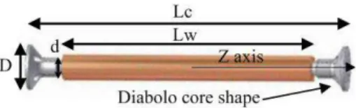
When a “diabolo” core is used (Coillot et al., 2007) the ap-parent permeability is increased thanks to the magnetic flux
Figure 1. Diagram of an induction sensor with a diabolo core shape.
concentrators (shown in Fig. 1). In this work the various fer-romagnetic core shapes will be linked to the one of the di-abolo cores. In the case of didi-abolo core shape the apparent permeability equation becomes
µapp-diab=
µr
1+Nz(m′)d 2 D2(µr−1)
, (4)
where Nz(m′) is the magnetometric demagnetizing coeffi
-cient for a cylinder of length-to-diameter ratiom′=Lc/D,
whiled2/D2 represents the surface ratio between the centre and the end surfaces of the core.
In the case of ferromagnetic core induction sensor, the in-ductance equation given in Tumanski (2007) is recalled here:
Ł=λN2µ0 µappS
Lc
, (5)
whereS is the ferromagnetic core section,µ0 is the vacuum permeability andλ=(Lc/Lw)2/5 is a correction factor pro-posed in Lukoschus (1979).
2.2 Transfer function of the induction sensor
Using a ferromagnetic core exhibiting an apparent perme-abilityµapp, the induced voltage is expressed (in harmonic regime at the pulsationω) as
e=−jωNSµappB, (6)
wherejrepresents the unit imaginary number j2=
−1 andB
is the magnetic flux density. The electrokinetic modelling as-sumes that the induced voltage is in series with the resistance and the inductance, while the accessible voltage (V) is mea-sured at the capacitance terminals. Thus, the transmittance (T(jω)) is given by the following equation:
T(jω)=V
B =
−jωNSµapp
1−LCω2+jRCω. (7)
natural electromagnetic waves are measured, such as earth-quake measurements, whistler observations and space plas-mas. In such applications two kinds of electronic condition-ers are classically implemented: feedback flux amplificondition-ers or current amplifiers. In both cases, the transfer function will be flattened over about 3 to∼6 decades.
2.3 Noise-equivalent magnetic induction
Noise-equivalent magnetic induction (NEMI), expressed in
T
√
(Hz), is the relevant quantity to determine the ability of the magnetometer to measure weak magnetic fields. The NEMI is defined as the square root of the total power spectrum density of the input reffered noise (PSDINPUT) related to the transfer function modulus (T(jω)):
NEMI=
s
PSDINPUT
|T(jω)2|, (8)
where
PSDINPUT=4kT R+e2PA+(ZiPA)2, (9)
wherekis the Boltzmann constant,T is the temperature,Z
is the impedance and the electronic amplifier noise param-eters areePA=4 nV/√(Hz) andiPA<20 fA/√(Hz). Due to the low-frequency context, the current noise contribution (i.e. (ZiPA)2≪ePA) will be neglected.
3 Cubic induction sensor
3.1 Description of the sensor configuration
The cubic magnetometer proposed in Dupuis (2003) com-bines multiple induction sensors to form a cubic array (a di-agram and a prototype are shown in Fig. 2). The advantages claimed by the author are the increase in sensitivity and the reduction of the self-inductance since the required turn num-ber can be dispatched between the different edges. The cores are implemented in such a way that they are not coupled on the magnetic point of view but are connected in series on the electrical point of view. The sensitivity benefit is related to an increase in the apparent permeability. Our current goal is to confirm the behaviour of this original induction sensor configuration, briefly presented in Coillot and Leroy (2012), through experimental measurements with a prototype and the validation of the apparent permeability equation with the aim of comparison to classical induction sensors.
The edges of the cubic induction sensor are constituted by cylinder ferromagnetic cores of lengthLcand diameterd. Due to the cubic shape, the demagnetizing coefficients are the same in the three directions:
Nx=Ny=Nz=
1
3. (10)
Figure 2. Cubic induction sensor diagram (left picture) and 85 cm×85 cm×85 cm prototype (right picture).
The flux caught by the square area face is distributed be-tween the four ferromagnetic cores with a ratio correspond-ing to the surface ratio. The equation of the apparent per-meability of the cubic sensor (µapp-cub) is then obtained as a special case of the diabolo core apparent permeability for-mula (given by Eq. 4) where the demagnetizing coefficient is equal to 13 and the surface ratio isL2
c/(4×πd2/4); this leads to
µapp-cubx,y,z=
µr
1+Nx,y,z(µr−1)πd 2 L2
c
. (11)
For sufficiently high relative permeability (i.e.µr≫1 and
Nµr≫1), we can simply write
µapp-cubx,y,z≃ 3L2
c
πd2. (12)
The previous formula is different from the one presented in Coillot and Leroy (2012), which is only valid for rods with square sections (despite what is claimed in the article).
3.2 Experimental results
A prototype cubic induction sensor has been built to eval-uate the modelling of the apparent permeability and the im-pact on the resonance frequency. The design equations which have been used are directly derived from the one of the clas-sical induction sensors presented above. The design parame-ters (turns number, core diameter, copper wire diameter) have been computed to allow the prototype to reach a NEMI value close to 0.7 pT/√Hz at 10 Hz. The design parameters of the prototype are summarized in Table 1.
The cubic induction sensor prototype (left picture in Fig. 2) is a 85 cm×85 cm×85 cm cube. A ferrite cube has been mounted at each corner of the cube to ensure a closed ferromagnetic path. The ferromagnetic material used for the ferromagnetic parts is B1 ferrite material whose initial rela-tive permeability is typically about 2500. The ferromagnetic core has been wound in a single direction. In this direction, each of the four edges were wound with 8000 turns of 70µm
Table 1. Design parameters of the cubic induction sensor pro-totype for a NEMI goal: 0.7 pT/√(Hz) at 10 Hz, assuming ePA=
4 nV/√(Hz) andiPA=20 fA/
√ (Hz).
Cylinder core length (Lcin mm) 85
Core diameter (din mm) 4
Copper wire turns (Nper core) 8000
Wire diameter (dwin mm) 0.07
Layer number nl=4
Winding length (Lwin mm) 80
Resistance (RinΩ) 1300
Apparent permeability (µapp-cub) 354
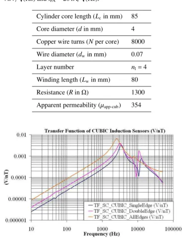
Figure 3.Transfer function of the cubic induction sensor: one edge (dark blue), two edges (pink) and four edges (orange curve).
magnetic field point of view in order to cancel the mutual induction between edges. It results that from a single edge to four edges, an increase in inductance by a ratio of 4 is ex-pected (instead of 16 when inductances are magnetically cou-pled). The transfer function has been measured in three cases: single edge, double edges and four edges. This shows that the increase in gain (before the resonance) is proportional to the edge number and is multiplied by almost 4 from a single edge to four edges. The reason why the ratio between four edges and single edges is not precisely equal to 4 could be explained by a unbalanced magnetic path (namely the fluxes seen by each edge are not exactly identical). The resonance frequency varies weakly (from 3400 Hz for the single edge to 2700 Hz for four edges). This could be related to the fact that when the edges are connected together, the total induc-tance increases, while the total capaciinduc-tance decreases; conse-quently the resonance frequency does not vary significantly. This property is of great interest for the design of wide-band and compact induction sensors. However, the multiple res-onance next to the main resres-onance could make the use of feedback flux or current amplifiers difficult.
The apparent permeability deduced from the measure-ment (cf. Fig. 3) is µapp-cub-meas=354, while the numerical application of Eq. (11) gives a rather close approximation (µapp-cub=368), which validates our modelling attempt.
3.3 Discussion
In order to evaluate the benefit of the cubic induction sensor, we will compare its apparent permeability and inductance to the one of a cylinder core induction sensor of the same length (Lc) and diameter (d). Under the ellipsoid shape approxima-tion, its demagnetizing coefficient is given by Eq. (3). Thus the long cylinder’s apparent permeability (Eq. 2) can be writ-ten (assumingNz(m)µr≫1)
µapp= 1
Nz(m) =L
2 c
d2 1 ln(2Lc
d)−1
. (13)
The comparison between the cubic sensor and the usual induction sensor can be done through the ratio between their apparent permeability (from Eqs. 12 and 13), which leads to
µapp-cub
µapp =3
π(ln(2
Lc
d )−1). (14)
This comparison suggests that the cubic induction sensor has a higher apparent permeability than the single rod since
Lc
d ≫1. For example, for aLc/d ratio equal to 10, the cubic
sensor apparent permeability will be about two times higher than the one of the single rod.
4 Orthogonal induction sensor
4.1 Description of the sensor configuration
In an orthogonal search coil, a helical core (shown in Fig. 4) is used to enhance the flux catched by each turn. Because of the two ferromagnetic discs (diameterD) mounted at the ends of the helicore (whose total length isLc), and assuming a high relative permeability (µr), the external magnetic flux is canalized by the ends of the core and driven through each fer-romagnetic core turn. The ferfer-romagnetic turns are assumed to be square with sided.
To compute the induced voltage, we have to consider the angle between the normal vector of the coil turn section and the direction of the magnetic field inside the helicore; this angle (ϕ), called the helix angle, is defined as
ϕ=arctan b
a
!
. (15)
where the pitch of the helicore (2πb) is determined as
2πb=Lw
n , (16)
Figure 4.Diagram of the orthogonal induction sensor.
ForNturns of coil surrounding thencore section, the in-duced voltage (ehc) becomes
ehc=−jωNnµapp-hcBScos(ϕ), (17)
whereS is the section of the core turns (equal tod2) and µapp-hc is the apparent permeability of the helical ferromag-netic core.
This apparent permeability is directly derived from the for-mula of the diabolo core, given in Eq. (4). In that caseNz(m′)
is the demagnetizing coefficient for the cylinder of length-to-diameter ratiom′=L/Dand d2
πD2/4 is the surface ratio be-tween the square section of the core turns and the end discs’ section of the core.
Finally, the sensitivity of the induction sensor, assuming low-frequency operation (ω≪ω0), is obtained:
|T(jω)|=|ehc
B |=ωNnµapp-hcScos(ϕ). (18)
The resistance of the coil (Rhc) is a derivation of the Eq. (1), while the inductance formula is intuitively obtained:
Łhc=λ(nN)2µ0
µapp-hcScos(ϕ)
l . (19)
The NEMI of the orthogonal induction sensor can be esti-mated using Eq. (20).
NEMIhc=
q
4kT Rhc+e2PA ωNnµapp-hcScos(ϕ)
. (20)
4.2 Experimental results
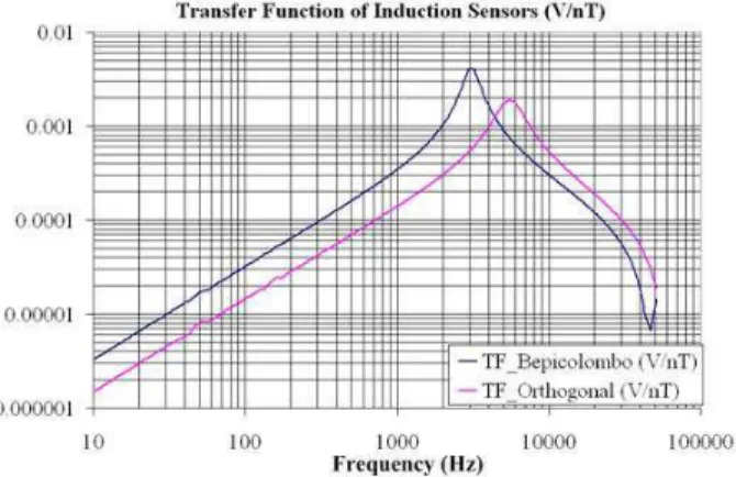
By using the previous set of equations we have determined the number of turns of an orthogonal sensor to get the same NEMI as the diabolo core sensor designed within the context of the BepiColombo space mission (namely 2 pT/√(Hz) at 10 Hz from Coillot et al., 2010). The following set of design parameters was chosen:dw=140µm, Lc=100 mm,n=28,
d=3 mm, DO=20 mm, a=3.5 mm and Lw=90 mm. The design result led to a 400-turn coil on a single layer. The
Figure 5.Picture of the orthogonal induction sensor prototype.
Figure 6. Transfer function of the orthogonal induction sensor (pink curve) versus that of the BepiColombo sensor (blue curve).
expected sensitivity at 10 Hz is about 2300 V/T, while the ex-pected resistance should be four times lower than the one of the BepiColombo sensor (cf. Table 2). The orthogonal induc-tion sensor prototype is shown in Fig. 5. It can be noticed that the coil normal direction is orthogonal to the direction of the magnetic field.
The advantage of the helicore is that the sensitivity crite-rion can be met with a small number of turns; the drawback is the difficulty in winding the core.
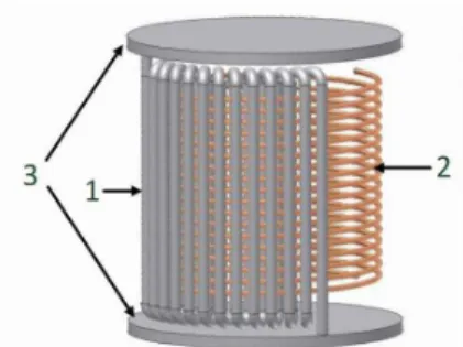
Figure 7.Diagram of the coiled-core induction sensor. (1) shows the ferromagnetic coil, (2) the conductive coil and (3) the ferromag-netic discs.
the orthogonal induction sensor is the higher resonance fre-quency, which permits extension of the frequency range of the measurement. The helical angle could reduce the perfor-mance, and thinner cores (on the helicore part) would reduce this angle and consequently increase the sensitivity. Lastly, the resonance frequency is lower than expected, which indi-cates that some leakage flux between core turns occurs. The use of a ferromagnetic wire to design an orthogonal induc-tion sensor could solve the main problems encountered with the ferrite core.
5 Coiled-core induction sensor
5.1 Description of the sensor configuration
The coiled-core induction sensor, presented in Fig. 7, con-sists of ann-turns ferromagnetic wire (part 1) coiled around an ncoil-turns winding (part 2) made of conductive material like copper or aluminium. Similarly to the classical insulated conductive wire used to make the classical winding, the fer-romagnetic wire should be insulated to leave a space between turns as to avoid a short-circuited magnetic path.
A ferromagnetic disc (part 3), acting as magnetic concen-trators, is mounted at each end of the ferromagnetic wire in order to canalize the magnetic field. As a result, the mag-netic field “flows” through the ferromagmag-netic wire and each conductive coil turn “sees”ntimes the derivative of the flux of the ferromagnetic coil turns. The advantage of such a sen-sor is quite obvious, but we propose a modelling attempt to convince the reader of the potential interest of this theoretical sensor.
5.2 Modelling of the coiled-core induction sensor Let us consider a copper winding withN turns wound on a diameter Dcoil made with a conductive wire of resistivityρ and diameterdwon a length Lw. Similarly to the resistance formula of the induction sensor (cf. Eq. 1), the winding
re-sistance of the coiled-core (Rcc) sensor is expressed as
Rcc=4ρN
Dcoil+N(dw+2t)2/Lw
d2 w
. (21)
On the one hand, the available area to coil the ferromag-netic wire is given by
Scoil= πD2coil
4 . (22)
On the other hand the core section for a single wire is given by
Score= πd2
4 . (23)
For a given core-coil filling factorkf (a value of≃0.9 is considered for the design example), the coil-core number (n) is deduced:
n=kfScoil
Score
. (24)
In this relation we assume that the cored coil could be distributed on many layers inside the coil winding area. Let us now consider the sensor length Lc and the diameter of the ferromagnetic discsDO, the length-to-diameter ratio be-ing m′′=L
c/DO. The apparent permeability, derived from Eq. (4), can be expressed as
µapp-cc=
µr
1+Nz(m′′)d 2 D2 O
(µr−1)
. (25)
The induced voltage modulus and the sensitivity of the in-duction sensor(assuming low-frequency operation (ω≪ω0)) are given by Eqs. (26) and (27) respectively:
ecc=NnScoreµapp-ccωB, (26)
|T(jω)|=ecc
B =NnScoreµapp-ccω. (27)
The NEMI equation for the coiled-core sensor is
NEMIcc=
q
4kT Rcc+e2PA
NnScoreµapp-ccω
. (28)
Similarly to the orthogonal induction sensor, a design at-tempt is performed (we choose the following set of design parameters:dw=70µm,L=20 mm,d=1 mm,DO=20 mm andLw=18 mm). The electronic amplifier noise parameters (ePA and iPA) remain identical to previous cases. Because of the compactness of the coiled-core sensor (L=DO⇒
m′′≈1), a demagnetizing factorNz(m′′)=1/3 was
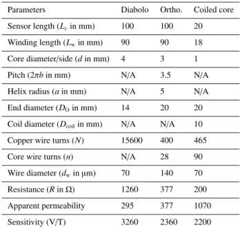
Table 2.Design parameters for diabolo, orthogonal and coiled-core induction sensors for an equal NEMI goal: 2 pT/√(Hz) at 10 Hz, assumingePA=4 nV/
√
(Hz) andiPA=20 fA/
√ (Hz).
Parameters Diabolo Ortho. Coiled core
Sensor length (Lcin mm) 100 100 20
Winding length (Lwin mm) 90 90 18
Core diameter/side (din mm) 4 3 1
Pitch (2πbin mm) N/A 3.5 N/A
Helix radius (ain mm) N/A 5 N/A
End diameter (DOin mm) 14 20 20
Coil diameter (Dcoilin mm) N/A N/A 10
Copper wire turns (N) 15600 400 465
Core wire turns (n) N/A 28 90
Wire diameter (dwinµm) 70 140 70
Resistance (RinΩ) 1260 377 200
Apparent permeability 295 377 1070
Sensitivity (V/T) 3260 2360 2200
This solution, which remains theoretical, could permit for strong reduction in the size of the sensor for a given sen-sor sensitivity. For the considered design, it suggests that a coiled-core induction sensor could be five times smaller than a classical induction sensor. The availability of windable fer-romagnetic wire is the weakness of this conceptual sensor.
6 Conclusions
The three induction sensors reported in this work offer new possibilities for improvements. We believe that the coiled-core induction sensor is the most promising one even if it remains theoretical as the prototype has not been built. Its manufacturing is strongly dependent on the availability of coilable and insulated ferromagnetic wire. Nevertheless, the orthogonal induction sensor and the coiled-core one are sim-ilar. The orthogonal induction sensor prototype has allowed for confirming the predicted performance, which provides good confidence concerning the real wound-core sensor per-formance. These three induction sensors could be adapted to enhance other magnetic sensors, especially fluxgates and gi-ant magneto-impedance (GMI). For instance, in the case of the GMI, the excitation current could flow through the ferro-magnetic wire, while the conductive winding could be used as a pick-up coil. The closeness of the ferromagnetic wire could enhance the skin effect by means of the proximity ef-fect, which could permit having high GMI ratio even at low frequency.
Acknowledgements. The authors would like to thank CNES (Centre National d’Etudes Spatiales), which has funded the proto-type manufacturing within the context of a spacecraft mission study.
Edited by: B. Jakoby
Reviewed by: two anonymous referees
References
Bozorth. R. M. and Chapin, D.: Demagnetizing factors of rods, J. Appl. Phys., 13, 320–327, 1942.
Coillot, C. and Leroy, P.: Induction Magnetometers: Principle, Mod-eling and Ways of Improvement, Magnetic Sensors – Princi-ples and Applications, edited by: Kuang, K., ISBN: 978-953-51-0232-8, InTech, 2012.
Coillot, C., Moutoussamy, J., Leroy, P., Chanteur, G., and Roux, A.: Improvements on the design of search coil magnetometer for space experiments, Sens. Lett., 5, 167–170 2007.
Coillot, C., Moutoussamy, J., Lebourgeois, R., Ruocco, S., and Chanteur, G.: Principle and performance of a dual-band search coil magnetometer: A new instrument to investigate fluctuating magnetic fields in space, IEEE Sens. J., 10, 255–260, 2010. Dupuis, J. C.: Optimization of a 3-AXIS Induction Magnetometer
for Airbone Geophysical Exploration, Master of Science in Egi-neering, University of New Brunswick, 2003.
Grosz, A. and Paperno, E.: Analytical Optimization of Low-Frequency Search Coil Magnetometers, IEEE Sens. J., 12, 2719– 2723, 2012.
Grosz, A., Paperno, E., Amrusi, S., and Liverts, E.: Integration of the electronics and batteries inside the hollow core of a search coil, J. App. Phys., 107, 09E703–E709E703-3, 2010.
Korepanov, V. and Pronenko, V.: Induction Magnetometers – De-sign Peculiarities, Sensors and Transducers Journal, 120, 92– 106, 2010.
Lichtenberger, J., Ferencz, C., Bodnar, L., Hamar, D., and Stein-bach, P.: Automatic whistler detector and analyzer system, J. Geophys. Res., 113, 2156–2202, 2008.
Lukoschus, D.: Optimization theory for induction-coil magnetome-ters at higher frequencies, IEEE T. Geosci. Elect., GE-17, 56–63, 1979.
Osborn, J. A.: Demagnetizing factors of the general ellipsoids, 67, 351–357, 1945.
Ozaki, M., Yagitani, S., Takahashi, K., and Nagano, I.: Develop-ment of a new portable Lightning Location System, IEICE Trans. Commun., E95-B, No. 1, January 2012.
Ozaki, M., Yagitani, S., Takahashi, K., and Nagano, I.: Dual-Resonant Search Coil for Natural Electromagnetic Waves in the Near-Earth Environment, IEEE Sens. J., 13, 644–650, 2013. Prance, R. J., Clarck, T. D., and Prance, H.: Ultra low noise
in-duction magnetometer for variable temperature operation, Sen-sor. Actuator., 85, 361–364, 2000.
Rhouni, A., Sou, G., Leroy, P., and Coillot, C.: A Very Low 1/f Noise and Radiation-Hardened CMOS Preamplifier for High Sensitivity Search Coil Magnetometers, IEEE Sens. J., 13, 159– 166, 2012.
Ripka, P.: Magnetic sensors and magnetometers, Ed. Artech House, 2000.
magnetometer for THEMIS, Space Sci. Rev., 141, 265–275, 2008.
Seran, H. C. and Fergeau, P.: An optimized low frequency three axis search coil for space research, Rev. Sci. Instrum., 76, 044502– 0044502-9, 2005.
Shimin, F., Suihua, Z., and Zhiyi, C.: A very low noise preamplifier for extremely low frequency magnetic antenna, Journal of Semi-conductors, 34, 075003–075003-5, 2013.
Sudduth, K. A., Drummond, S. T., and Kitchen, N. R.: Accuracy is-sues in electromagnetic induction sensing of soil electrical con-ductivity for precision agriculture, Comput. Electron. Agr., 31, 239–264, 2001.
Tumanski, S.: Induction coil sensors – A review, Meas Sci. Tech-nol., 18, R31–R46, 2007.