Paradoxical Effect
Ye Ye, Lu Wang*, Nenggang Xie*
Department of Mechanical Engineering, Anhui University of Technology, Anhui, People’s Republic of China
Abstract
Parrondo’s games were first constructed using a simple tossing scenario, which demonstrates the following paradoxical situation: in sequences of games, a winning expectation may be obtained by playing the games in a random order, although each game (game A or game B) in the sequence may result in losing when played individually. The available Parrondo’s games based on the spatial niche (the neighboring environment) are applied in the regular networks. The neighbors of each node are the same in the regular graphs, whereas they are different in the complex networks. Here, Parrondo’s model based on complex networks is proposed, and a structure of game B applied in arbitrary topologies is constructed. The results confirm that Parrondo’s paradox occurs. Moreover, the size of the region of the parameter space that elicits Parrondo’s paradox depends on the heterogeneity of the degree distributions of the networks. The higher heterogeneity yields a larger region of the parameter space where the strong paradox occurs. In addition, we use scale-free networks to show that the network size has no significant influence on the region of the parameter space where the strong or weak Parrondo’s paradox occurs. The region of the parameter space where the strong Parrondo’s paradox occurs reduces slightly when the average degree of the network increases.
Citation:Ye Y, Wang L, Xie N (2013) Parrondo’s Games Based on Complex Networks and the Paradoxical Effect. PLoS ONE 8(7): e67924. doi:10.1371/ journal.pone.0067924
Editor:Rodrigo Huerta-Quintanilla, Cinvestav-Merida, Mexico
ReceivedNovember 9, 2012;AcceptedMay 23, 2013;PublishedJuly 2, 2013
Copyright:ß2013 Ye et al. This is an open-access article distributed under the terms of the Creative Commons Attribution License, which permits unrestricted use, distribution, and reproduction in any medium, provided the original author and source are credited.
Funding:This project was supported by Ministry of Education, Humanities and Social Sciences research projects (11YJC630208 and 13YJAZH106), and the Natural Science Foundation of Anhui Province of China (Grant No.11040606M119). The funders had no role in study design, data collection and analysis, decision to publish, or preparation of the manuscript.
Competing Interests:The authors have declared that no competing interests exist.
* E-mail: xienenggang@aliyun.com (NX); wanglu@ahut.edu.cn (LW)
Introduction
Parrondo’s games can produce a paradoxical effect that alternating plays of two losing games can produce a winning game. Parrondo’s original games [1] involve two games, A and B. The player has some capital, which is increased by one with a probability of winning p1and decreased by one with a probability 1-p1 in game A. Game B is slightly more complicated, and the rules are that if the capital is a multiple of an integer M, the probability of winning is p2.If it is not, the probability of winning is p3.
Game A is a losing strategy if p1,0.5. Harmer et al. [2] showed that game B is a losing strategy when the inequality
(1{p2)(1{p3)M{1
p2p3M{1
w1holds, and the combined game A+B is a
winning strategy when the inequality (1{q2)(1{q3) M{1
q2q3M{1
v1
holds, whereq2~pp1z(1{p)p2,q3~pp1z(1{p)p3, and p is the
probability of playing game A. An example of the parameters that satisfy the previous inequalities was given by [1] as follows: p1= 0.5-e, p2= 0.1-e, p3= 0.75-e, M = 3, p = 0.5 and e= 0.005. Notice that wheneis zero, game A is a fair game (i.e., it is neither losing nor winning on average).
Parrondo’s paradox has been confirmed by computer simula-tions, the Brownian ratchet and the discrete-time Markov chain [2–4]. In addition, the Parrondo effect has inspired the studies of the negative-mobility phenomena [5], the reliability theory [6], the
noise-induced synchronization [7] and the controlling chaos [8]. In biological systems, Parrondo’s paradox may be related to the dynamics of gene transcription in GCN4 protein and the dynamics of transcription errors in DNA [2]. Moreover, Parrondo’s paradox has been studied in various interesting scenarios involving population genetics [9–12]. In the stock market, Boman et al. [13–14] used a Parrondian game framework as a toy model to study the dynamics of insider information. Parrondo’s paradox not only can be used to explain a large number of nonlinear phenomena [4] but also presents its own rich non-linear characteristics. Recent work [15] has shown that Parrondo’s games exhibit fractal patterns in their state space.
the engineering literature it is known that individually unstable systems can become stable if coupled together [16]. In the theory of granular flow, drift can occur in a counterintuitive direction. For instance, the ‘‘Brazil nut effect’’ [17–18] has shown that the large Brazil nuts rise to the top when you shake a bag of mixed nuts. In the area of mathematics, Pinsky and Scheutzow [19] have shown that switching between two transient diffusion processes in random media can form a positive recurrent process, which can be viewed as a continuous-time version of Parrondo’s games. Masuda and Konno [11], who studied the Domany-Kinzel probabilistic cellular automata, concluded that alternating two supercritical dynamics resulted in the subcritical dynamics in which the population died out. Almeida et al. [20] have proposed a case that ‘‘chaos+chaos = order’’, where the periodic mixing of two chaotic dynamics resulted in an ordered dynamics under certain circumstances. Therefore, the dynamic mechanisms similar to Parrondo’s games exist behind the counterintuitive phenomenon produced by the two mixed systems (processes, states). One system plays the ‘‘ratcheting’’ role, and the other plays the ‘‘agitating’’ role. The key to study these counterintuitive phenomena is to analyze the ‘‘ratcheting’’ role. By analyzing the phenomena such as the Brownian ratchet, the Brazil nut effect, the longshore drift on a beach, the buy-low sell-high process in stock-market trading and the two-girlfriend paradox, Abbott [21] demonstrated that various ‘‘ratcheting’’ mechanisms were caused by the asymmetries of space, friction, information, money and time.
The structure of game B in Parrondo’s original games has two branches, which depend on the modulus of the capital. Such dependence limited the application of the games in practice. Therefore, Parrondo et al. [3] modified game B and devised a new structure that depended on the recent history (t-2,t-1) of wins and losses. The modified game B had four branches: (lose, lose), (lose, win), (win, lose) and (win, win). This new structure increased the region of the parameter space where the Parrondo’s paradox occurred. The theoretical analysis demonstrated that the para-doxical space based on the history-dependent model was 50 times larger than the original version [15].
The above variations of game B, which is capital-dependent or history-dependent, have been introduced into Parrondo’s games. Toral [22] and Mihailovic [23–24] proposed a structure of game B that depended on the neighboring players, who surrounded the player whose turn it was to play the game. A remarkable difference was that an ensemble ofNplayers was considered instead of only one player. Each one occupied a certain space. For any playeri, all of its surrounding neighbors composed its spatial niche. At present, there are networks of a one-dimensional line and a two-dimensional lattice, which connect N players. For the one-dimensional line, the neighbors of playeri are i-1 and i+1. I–1 andi+1 have four different winning and losing states, which are (0 0), (0 1), (1 0) and (1 1), where 0 denotes a losing state, and 1 denotes a winning state. Therefore, the structure of game B consists of four branches. The probability of winning in each branch for playeriisp0, p1, p2and p3respectively. For the two-dimensional lattice, the four neighbors of player i have the following five different winning and losing states (here, the positions of the winning and losing states of the neighbors are not distinguished): (1) all the four neighbors are in the losing states, that is, (0000); (2) one neighbor is in the winning state, and the other three neighbors are in the losing states, that is, (1000); (3) two neighbors are in the winning states, and the other two neighbors are in the losing states, that is, (1100); (4) three neighbors are in the winning states, and one neighbor is in the losing state, that is, (1110); (5) all the four neighbors are in the winning states, that is, (1111). Therefore, the structure of game B consists of five branches. The probability of winning in each branch for the playeriisp0,p1,p2,p3andp4respectively.
Because the actual networks are complex, there are many types of topologies, such as random graphs, small-world networks and scale-free networks. However, the above two structures of game B cannot be extended directly to arbitrary topologies, where the number of the neighbors of the nodes cannot be maintained consistently. Therefore, we want to design a structure of game B that can be applied to arbitrary topologies, which means a structure of game B that can be applied to the nodes with different degrees. Toyota [25] proposed a construction method for game B Figure 1. The structure of game B based on arbitrary topologies.
in scale- free networks, where each player on a network played a game L when there was R or more winners in the neighborhood connected to the player and played a game W otherwise in game B. The simulation results and the theoretical studies showed that
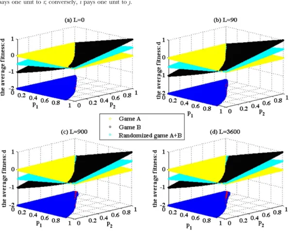
Parrondo’s paradox might not occur. Here, based on the spatial neighboring environment, the paper proposes a structure of game B to be applied in arbitrary topologies. The results show that Parrondo’s paradox can occur. Moreover, the size of the region of Figure 2. The degree distributions progressively changing from a two-dimensional network to a random graph.The size of the network is 900. The number of rewiring timesLis 0, 90, 900 and 3600 respectively.L= 0 corresponds to a two-dimensional lattice. The degree distribution of the network is addistribution and the degree of all nodes is four. The node degree of the network progressively changes to a Poisson distribution with the increment ofL.The average degree of the nodes remains at four during this process.
doi:10.1371/journal.pone.0067924.g002
Figure 3. The degree distributions progressively changing from a random graph to a scale-free network.The network size is 900. The parameterais 1.0, 0.7, 0.3 and 0.0 respectively.a= 1 corresponds to a random graph. The node degree of the network satisfies a Poisson distribution. With the decrease ofa, the node degree of the network gradually changes to a power-law distribution.a= 0 corresponds to a scale-free network. The
the parameter space that elicits Parrondo’s paradox depends on the heterogeneity of the degree distributions of the networks. A higher heterogeneity of the degree distributions of the networks produces a larger region of the parameter space where the strong paradox occurs.
Model
In this article, Parrondo’s model based on arbitrary topologies is shown in Figure 1. The model is composed of two games, A and B. Consider complex networks composed of N nodes. The game modes include playing game A and game B individually and playing a randomized game A+B. The randomized game A+B means a probabilistic sequence of games A and B. The dynamic processes of the randomized game A+B are as follows: for each round of the game, one node ‘i’ is chosen at random fromNnodes to play game A (with a probabilityp) or game B (with a probability 1-p).
A Zero-sum Game between Individuals–Game A
Game A is used to represent the competition behavior between the individuals in the networks, which is designed to be a zero-sum game. It has no impact on the total capital of the population, but it changes the capital distributions among the population. When game A is played, we need to randomly choose a nodejfrom the neighboring nodes that are connected with i. The winning probabilities of nodesiandjare 0.5, respectively. Wheniwins,j
pays one unit toi; conversely,ipays one unit toj.
The Construction of Game B
We consider the following two conditions when constructing game B: (1) The structure of game B needs several branches to form the ‘‘ratcheting’’ mechanism. (2) The structure of game B needs to be applied to the individuals with an arbitrary number of neighbors. We must avoid the influence of the number of neighbors while constructing the branches. Based on these two considerations, game B has two branches, which are generated according to the capital of nodeiand its neighbors. In branch one, when the capital of node i is less than or equal to the average capital of all of its neighbors, the winning probability isp1; in branch two, when the capital of nodeiis greater than the average capital of all of its neighbors, the winning probability isp2. Game B can also be constructed in other forms that are applicable to any networks. Therefore, the results and the related conclusions of this paper are obtained based on the Parrondo’s model shown in Figure 1.
Computer Simulations
We perform the following computer simulations based on Parrondo’s model in complex networks.
Based on the needs of computer simulations, we define the average fitness of the populationdas follows:
d(t)~W(t)
T:N
ð1Þ
Figure 4. Simulations based on the networks, which progressively change from a two-dimensional lattice to a random network.The population sizeNis 900. The average degree of the network is four, and the average number of playing timesTof each individual is 100. The probability of playing game A isp= 0.5. Play the games 30 times with different random numbers, and draw the corresponding figures according to the average results of the games. The blue area in the picture demonstrates the weak Parrondo’s paradox area, whereas the red denotes the strong area. Figures 4 (a), (b), (c) and (d) correspond to the networks with the rewiring times L = 0, 90, 900 and 3,600, respectively.
where:Nis the population size, andTis the average number of playing times for each individual. In this study, T= 100.
W(t)~P N i~1
Ci(t), which denotes the total capital of the population,
andCi(t) is the capital at time t (t[½0,TN) of individual i. The initial capital of all individuals is equal.
The condition under which the weak paradox occurs is as follows:
dðAzBÞ
wdð ÞB ð2Þ
The conditions under which the strong paradox occurs are as follows:
dðAzBÞ§0 ð3Þ
dð ÞB
v0 ð4Þ
wheredð ÞBanddðAzBÞrepresent the capital of games B and A +B in the steady state, respectively.
In the following section, we analyze three types of factors, including the heterogeneity of the degree distributions of the networks, the network size and the average degree of the network, and observe the influence of these factors on the paradoxical effect.
The Influence of the Heterogeneity of the Degree Distributions of the Networks on the Paradoxical Effect
To cleanly control the heterogeneity manipulation, we use the following two methods.
(1) In order to reflect the progressive changes from a dimensional lattice to a random graph, we start from a two-dimensional lattice and use the following rewiring mechanism to generate a random graph. The basic steps are as follows Figure 5. Simulations based on the networks, which progressively change from a random network to a scale-free network.The population sizeNis 900. The average degree of the network is four and the average number of playing timesTof each individual is 100. The probability of playing game A isp= 0.5. Play the games 30 times with different random numbers, and draw the corresponding figures according to the average results of the games. The blue area in the picture demonstrates the weak Parrondo’s paradox area, whereas the red denotes the strong area. Figures. 5 (a), (b), (c) and (d) correspond to the networks with the parametera= 1.0, 0.7, 0.3 and 0.0, respectively.
doi:10.1371/journal.pone.0067924.g005
Table 1.The average fitness and the proportion of playing branch two (from the two-dimensional lattice to the random network).
Game Modes L= 0 L= 90 L= 900 L= 3600
d proportion d proportion d proportion d proportion
Game B 0.0339 49.20% 0.0328 49.12% 0.0240 48.48% 0.0179 48.05%
Randomized game A+B 0.0187 49.47% 0.0186 49.44% 0.0172 49.25% 0.0166 49.15%
[26]: (a) generate an initial two-dimensional lattice; (b) randomly choose a node E and then randomly choose a node F from E’s neighbors. Break the connection between nodesEandF; (c) randomly choose two nodesGandHfrom the network and build a connection betweenEandGand a connection between F and H; (d) repeat steps (b) and (c)L
times. As the number of rewiring times (L) increases, the stochastic degree of the network increases. The node degree of the network progressively changes from addistribution to a Poisson distribution. Moreover, the average degree of the network remains at four. The number of rewiring timesLis the controlling index of the heterogeneity of the degree distributions. The corresponding degree distributions of the networks are shown in Figure 2 (wherekis the degree, andp(k) is the probability).
(2) To reflect the progressive changes from a random graph to a scale-free network, we use a model based on the degree distribution with adjustable parameters of the network and use the corresponding construction algorithm. The steps of the algorithm [27] are as follows: (a) growth. The initial network
consists ofNnodes, wherem0nodes are fully connected, and a setJ2is constituted; an unconnected setJ1is composed of (N -m0) isolated nodes. At each time step, choose a new node from J1. The new node has m edges connected with the other nodes. (b) Preferential attachment. The above new node’sm
edges are randomly linked to any other node from (N-1) nodes with a probability a (here, we have to avoid the multiple edges); then connect the nodes of the setJ2 by following a linear preferential-attachment strategy with the probability 1-a. After the connection is completed, we remove the new node
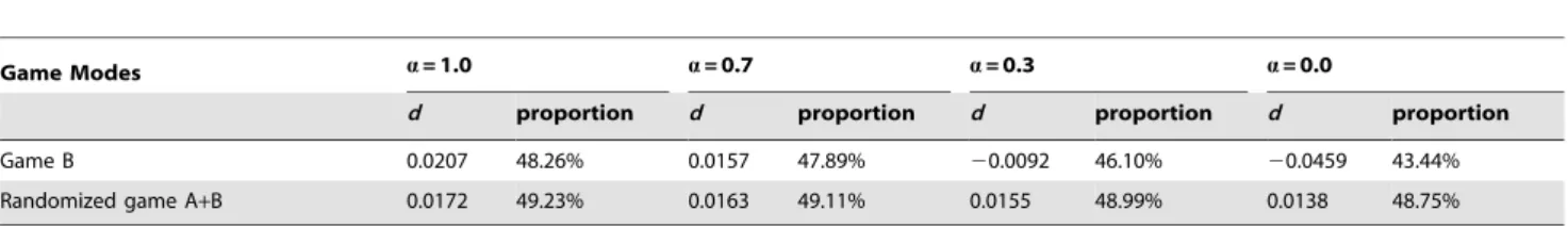
fromJ1and add it intoJ2. (c) AfterN-m0time steps, a series of networks are generated by controlling the parametera[½0,1, wherea= 0.0 corresponds to a scale-free network, anda= 1.0 corresponds to a random graph. With a decrease ina, the node degree changes progressively from a Poisson distribution to a power-law distribution, and the average degree of the network remains at four. The parameterais the controlling index of the heterogeneity of the degree distributions. Figure 3 shows the corresponding degree distributions of the networks. Table 2.The average fitness and the proportion of playing branch two (from the random network to the scale-free network).
Game Modes a= 1.0 a= 0.7 a= 0.3 a= 0.0
d proportion d proportion d proportion d proportion
Game B 0.0207 48.26% 0.0157 47.89% 20.0092 46.10% 20.0459 43.44%
Randomized game A+B 0.0172 49.23% 0.0163 49.11% 0.0155 48.99% 0.0138 48.75%
doi:10.1371/journal.pone.0067924.t002
Figure 6. The relationship between the degree and the capital (based on the BA scale-free network).The population sizeNis 10, 000. The average degree of the network is four and the average number of playing timesTof each individual is 100. The probability of playing gameAis
p= 0.5. The probabilities of winning in branch one and branch two of game B arep1= 0.175 andp2= 0.870, respectively. Play the games 1000 times
with different random numbers, and draw the corresponding figures according to the average results of the games. For the nodes with the same degree, the capital is averaged from all of these nodes.
The simulation results based on Parrondo’s model (shown in Figure 1) are given in Figures 4 and 5. These results demonstrate that the structure of game B proposed in the paper can produce Parrondo’s paradox based on the complex networks. Figure 4 shows that the results of Parrondo’s paradox change progressively from a two-dimensional lattice to a random network. As the number of rewiring times, L, increases, the node degree of the network gradually changes from a ddistribution to a Poisson
distribution. Moreover, the region of the parameter space where the strong paradox occurs (the red region in Figure 4) grows progressively. The region of the parameter space where the weak paradox occurs (the blue part in Figure 4) is divided into two regions by the red part. The characteristic of the large blue area on the left of the red region is0wdðAzBÞwdð ÞB. The characteristic of the small blue area on the right of the red region is
dðAzBÞwdð ÞBw0. With the increment of the rewiring times L, the blue area corresponding to dðAzBÞwdð ÞBw0 progressively grows. Figure 5 shows the results of Parrondo’s paradox progressively changing from a random network to a scale-free network. As the parametera decreases, the node degree of the network progressively changes from a Poisson distribution to a power-law distribution. In addition, the region of the parameter space in which the strong paradox occurs (the red region in Figure 5) grows progressively. Moreover, the region of the parameter space in which the weak paradox occurs (the blue part that corresponds todðAzBÞwdð ÞBw0, as shown in Figure 5) also grows. Therefore, the region of the parameter space where Parrondo’s paradox occurs is related to the heterogeneity of the degree distributions of the networks. A higher heterogeneity leads to a larger region of the parameter space where the strong or weak paradox occurs.
To analyze the mechanisms that elicit the paradox and the reason for the effect of the heterogeneity of the degree distributions of the networks, a set of specific parameters (p1= 0.175 and p2= 0.870) is chosen based on the results of Figures 4 and 5. We count the proportion of playing the favorable branch of game B, which is the number of times that the favorable branch of game B is played in comparison to the number of times that game B is played (for parametersp1= 0.175 andp2= 0.870, branch two is the favorable one). The results are shown in Tables 1 and 2.
Tables 1 and 2 show that (1) the proportion of playing the favorable branch of the randomized game A+B is larger than that of game B played individually, which shows that the ‘‘agitating’’ role of game A increases the chance to play the favorable branch; (2) when the heterogeneity of the degree distributions of the networks increases, for the given set of parameters (p1= 0.175 and p2= 0.870), first, the paradoxical effect is not produced (when L= 0, 90, 900 and 3,600 anda= 1.0,dð ÞBwdðAzBÞw0), then, the
weak paradox occurs (when a= 0.7, dðAzBÞwdð ÞBw0), and finally, the strong paradox occurs (when a= 0.3 and a= 0.0, dðAzBÞw0 and dð ÞBv0). The same changing trend is shown in Figures 4 and 5. The main reason for this finding is that when the heterogeneity of the degree distributions of the networks increases, the proportions of playing the favorable branch in both the randomized game A+B and game B decrease. However, the proportion of playing the favorable branch in game B decreases more significantly, from 48.26% (whena= 1.0) to 43.44% (when a= 0.0), whereas the proportion of playing the favorable branch in the randomized game A+B decreases less from 49.23% (when a= 1.0) to 48.75% (when a= 0.0). This asynchronous decline
shows that the ‘‘agitating’’ role of game A contributes to the increase of the opportunity to play the favorable branch. In
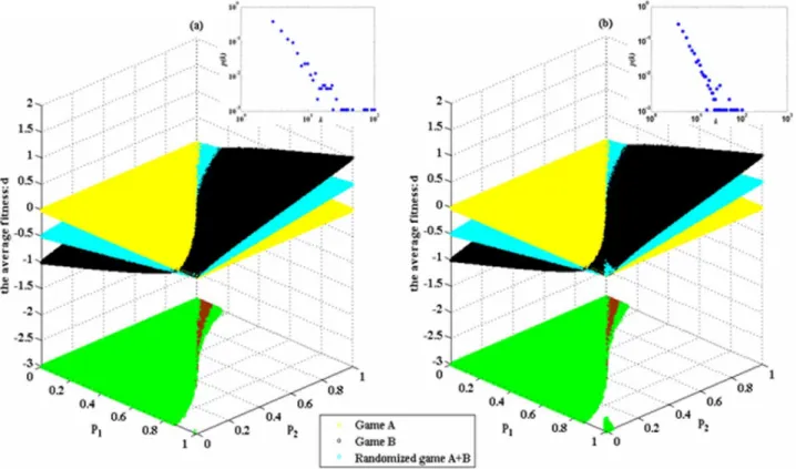
Figure 7. The influence of the network size on the Parrondo effect (based on the BA scale-free network).The average degree of the network is four and the average number of playing timesTof each individual is 100. The probability of playing game A isp= 0.5. Play the games 30 times with different random numbers, and draw the corresponding figures according to the average results of the games. The small window in the figure shows the degree distribution of the nodes. The green area in the figure represents the area of the weak Parrondo’s paradox, whereas the brown region denotes the strong area. The population sizeNof Figure 7 (a) is 400 and Figure 7 (b) is 10, 000, respectively.
addition, this contribution has a positive correlation with the heterogeneity of the degree distributions of the networks. Therefore, the asynchronous decline between the two results makes dð ÞBgradual changes from positive to negative, whereas
dðAzBÞ simultaneously remains positive. The given set of
parameters with which the paradox originally does not occur gradually evolves into the set of parameters with which the weak paradox or the strong paradox occurs. (3) whenL= 0, 90, 900 and 3,600 and a= 1.0, we find that each proportion of playing the favorable branch in game B is slightly smaller than that in the randomized game A+B, but dð ÞBwdðAzBÞ. The reason for this
result is that when we play the randomized game A+B, half of the total time is used to play the zero-sum game (i.e., game A). Although the proportion of playing the favorable branch in game B is smaller, the total time to play the favorable branch is more than that in the randomized game A+B (The total time of playing the unfavorable branch in game B is also more than that in the randomized game A+B). When the proportion of playing the favorable branch in game B is large enough, the corresponding gain is enough to offset the loss of playing the unfavorable branch. Therefore,dð ÞBwdðAzBÞ.
In the following section, we use a BA network as an example and attempt to explain the following questions from a micro level: (1) why does a higher heterogeneity of the degree distributions of the networks lead to a smaller opportunity to play the favorable branch in game B? (2) Why does the ‘‘agitating’’ role of game A increase the chance to play the favorable branch? (3) The ‘‘agitating’’ role of game A contributes to increasing the
opportunity to play the favorable branch. Then, why does this contribution have a positive correlation with the heterogeneity of the degree distributions of networks?
We choose p1= 0.175 and p2= 0.870 and perform the simulations on a BA network with 10,000 nodes. The results show that the average fitness values of the populationdof game B and the randomized game A+B are 20.0456 and 0.0141, respectively. Thus, the strong paradox occurs. The proportions of playing the favorable branch in game B and the randomized game A+B are 43.48% and 48.79%, respectively. Figure 6 shows the relationship between the node degree and the capital. From the figure, we observe that when game B is played individually, the positive relations exist between the node degree and the capital. A larger node degree corresponds to a larger capital. The capital of node degrees two and three is negative and the capital of the other node degrees is positive (because the number of nodes with degrees two and three accounts for 70% of the total amount of nodes, the average fitness of the population is negative). This result occurs because for parametersp1= 0.175 andp2= 0.870, when the capital of a node is less than the average capital of all of its neighbors, the niche of this node is not favorable (branch one of game B is played, and the probability of winning isp1= 0.175). Otherwise, if the average capital of all of the neighbors is less than or equal to the capital of a node, the niche of this node is favorable (branch two of game B is played and the probability of winning isp2= 0.870). Because the niche of the nodes with large degrees is mainly composed of nodes with small degrees, we assume that the capital of the nodes with small degrees is small. At the beginning of the game, because the number of the node degrees two and three
accounts for 70% of all nodes, the nodes with small degrees have a large chance of being chosen for the game. In addition, because the initial capital of all nodes is the same, according to the rules of game B, the node with a small degree chosen for the game will play branch one. Then, the probability of losing is large, which results in the capital decreasing. Therefore, in the initial stage of the game, this hypothetical situation is a large-probability event. Thus, the nodes with large degrees play the favorable branch two with a larger probability, which increases the capital of the nodes with large degrees. Therefore, the niche of the small-degree nodes that are connected to these large-degree nodes is further worsened (because the number of neighbors of the small-degree nodes is only two or three, the increment of the capital of the large-degree nodes causes the average capital of the niche to produce a comparatively obvious rise). Moreover, this result makes the small-degree nodes play the unfavorable branch one with a larger probability, which reduces the capital of the nodes with small degrees. The favorable niche of the nodes with large degrees and the unfavorable niche of the nodes with small degrees are constantly strengthened in the playing courses. Finally, a phenomenon is produced that the larger node degree corresponds to more capital, and the smaller node degree corresponds to less capital. Meanwhile, because the number of nodes with small degrees is far greater than the number of nodes with large degrees, the favorable niche of the nodes with large degrees and the unfavorable niche of the nodes with small degrees make the proportion of playing the favorable branch small. This situation, which is favorable for the nodes with large degrees and unfavorable for the nodes with small degrees, is quite obvious in the BA network. When the heterogeneity of the degree distributions of the networks decreases, this situation will be
weakened. The proportion of playing the favorable branch of the population will increase.
When the randomized game A+B is played, from Figure 6, we can observe that the node degree has no obvious relation with the capital, where the capital of the node degrees two and three, which account for 70% of the population, is positive (this result makes the average fitness of the population is positive). The reason for this result is the ‘‘agitating’’ role of game A. Because the nodes with large degrees and the nodes with small degrees will play a zero-sum game among them, the winning and the losing probabilities are the same. This process makes the nodes with small degrees have the chance of capital growth. Moreover, this process disrupts the strengthening process of the favorable niche of the nodes with large degrees and the unfavorable niche of nodes with small degrees. Even in a local area of the network, an inverse strengthening process may appear, where the unfavorable niche of the nodes with large or medium degrees (the average capital of the neighbors of the nodes with small degrees is large) and the favorable niche of the nodes with small degrees are formed (in this example, there is a phenomenon that the capital of nodes with degrees 49, 81, 83 and 97 is negative). Therefore, the ‘‘agitating’’ role of game A makes the nodes with small degrees increase the chance of playing the favorable branch in game B.
A higher heterogeneity of the degree distributions corresponds to a larger proportion of pairs of neighbors that are composed of large-degree nodes and small-degree nodes. Moreover, a higher heterogeneity of the degree distributions correspons to a larger probability that the nodes with large degrees and the nodes with small degrees play game A. Thus, this process disrupts the strengthening process that the favorable niche is formed by the
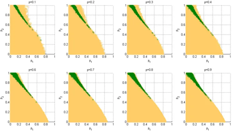
Figure 9. The influence of the probabilitypof playing game A on the Parrondo effect (based on the BA scale-free network).The population sizeNis 900. The average degree of the network is four and the average number of playing timesTof each individual is 100. Play the games 30 times with different random numbers, and draw the corresponding figures according to the average results of the games. The orange area in the figure represents the weak-paradox area, whereas the green region denotes the strong-paradox area.
nodes with large degrees and the unfavorable niche by the nodes with small degrees. Therefore, the ‘‘agitating’’ role of game A contributes to the increas of the opportunity to play the favorable branch, and this contribution positively correlates with the heterogeneity of the degree distributions of the networks.
The Influence of the Network Size on the Paradoxical Effect
In order to investigate the impact of the size of the scale-free network on the Parrondo effect, we maintain the same average degree of the network (i.e., four) and the same heterogeneity of the degree distributions of networks. The size of the scale-free network is reduced to N= 400 and expanded toN= 10,000, respectively. The results are shown in Figure 7. Comparing Figure 5 (d) with Figure 7 (a) and Figure 7 (b), we notice that the region of the parameter space where the strong or weak paradox occurs has no significant change with the expansion of the network size (in the region of the parameter space where the strong paradox occurs, the percentages of Figure 5(d), Figure 7(a) and Figure 7(b) are 1.71%, 1.74% and 1.72, respectively; in the region of the parameter space where the weak paradox occurs, the percentages of Figure 5(d), Figure 7(a) and Figure 7(b) are 50.38%, 50.46% and 50.53%, respectively). The reason for this result is that when the average degree of nodes remains unchanged, the expansion of the size of the scale-free network has not effectively changed the heterogeneity of the degree distributions of networks.
The Influence of the Average Degree of Networks on the Paradoxical Effect
In addition, in order to investigate the impact of the average degree of the scale-free network on the Parrondo effect, we maintain the same network size (i.e., N= 900) and the same heterogeneity of the degree distributions of networks. We increase the average degree of the scale-free network. The results are shown in Figure 8. We compare Figure 5 (d) (the average degree of the network is four) with Figure 8 (a) (the average degree of the network is 5.9867) and Figure 8 (b) (the average degree of the network is 7.9756). Then we notice that the region of the parameter space where the strong Parrondo’s paradox occurs slightly reduces (the percentages of Figure 5 (d), Figure 8(a) and Figure 8(b) are 1.71%, 1.37% and 1.17%, respectively) when the average degree of the network increases. When the size of the scale-free network remains unchanged, the increment of the average degree of the node has slightly reduced the heterogeneity of the degree distributions of networks. The region of the parameter space where the weak paradox occurs has no significant change (the percentages of Figure 5 (d), Figures 8 (a) and 8(b) are 50.38%, 50.37% and 50.40%, respectively). In addition, compar-ing Figure 5(d) with Figure 8(a) and Figure 8 (b) between the regions of p1R1 and p2R0, we notice that the region of the parameter space where the weak Parrondo’s paradox occurs increases with a small growth (the percentages of Figure 5 (d), Figure 8 (a) and Figure 8 (b) are 0%, 0.005% and 0.25%,
respectively) along with the increment of the average degree of the network. The capital corresponding to these areas is
dðAzBÞwdð ÞBw0.
The Influence of the Probabilitypof Playing Game A on the Paradoxical Effect
Finally, in order to reflect the effect of the probability p of playing game A, based on a scale-free network, we calculate the capital of the strong and weak regions that corresponds to different
pvalues, as shown in Figure 9. From Figures 9 and 5(d), we notice that when p#0.5, the strong paradoxical region gradually increases with the increment ofp. The weak paradoxical region of the upper part of the trapezoidal shape (which corresponds to
dðAzBÞwdð ÞBw0) gradually reduces with the increment of p, whereas the weak paradox region of the bottom part of the trapezoidal shape (which corresponds to0wdðAzBÞwdð ÞB) grad-ually increases with the increment ofp. Whenp.0.5, the strong paradoxical region has no obvious change with the increment ofp. With the increment of p, the weak paradoxical region that corresponds to dðAzBÞwdð ÞBw0reduces gradually, whereas the weak paradoxical region that corresponds to0wdðAzBÞwdð ÞB has no obvious change. Therefore, playing game A with a larger probability (p$0.5) is conducive to generating a strong paradox.
Conclusions
In this article, Parrondo’s model based on complex networks (shown in Figure 1) is proposed. Based on the spatial niche, a structure of game B is constructed, which can be applied to arbitrary topologies. The results show that Parrondo’s paradox occurs. Moreover, the region of the parameter space where Parrondo’s paradox occurs is related to the heterogeneity of the degree distributions of networks. A higher heterogeneity corre-sponds to a larger region of the parameter space where the strong paradox occurs. Therefore, the heterogeneity of the degree distributions of networks is conducive to the ‘‘agitating’’ mecha-nism. This mechanism may also cause most of the networks in reality to exhibit the high heterogeneity. In addition, the region of the parameter space where the strong or weak paradox occurs does not change significantly when the scale-free network expands. The region of the parameter space where the strong Parrondo’s paradox occurs slightly reduces when the average degree of the network increases. Moreover, playing game A with a larger probability is conducive to generating a strong paradox.
Acknowledgments
We thank the two reviewers and the editor for their valuable comments.
Author Contributions
Conceived and designed the experiments: NX. Performed the experiments: YY. Analyzed the data: LW. Wrote the paper: YY.
References
1. Harmer GP, Abbott D (1999) Losing strategies can win by Parrondo’s paradox. Nature 402(6764): 864–870.
2. Harmer GP, Abbott D, Taylor PG, Parrondo JMR (2001) Brownian ratchets and Parrondo’s games. Chaos 11(3): 705–714.
3. Parrondo JMR, Harmer GP, Abbott D (2000) New paradoxical games based on Brownian ratchets. Physical Review Letters 85(24): 5226–5229.
4. Arena P, Fazzino S, Fortuna L, Maniscalco P (2003) Game theory and non-linear dynamics: the Parrondo paradox case study. Chaos, Solitons & Fractals 17(2): 545–555.
5. Cleuren B, Van den Broeck C (2002) Random walks with absolute negative mobility. Physical Review E 65(3): 030101.
6. Crescenzo AD (2007) A Parrondo paradox in reliability theory. The Mathematical Scientist 32(1): 17–22.
7. Kocarev L, Tasev Z (2002) Lyapunov exponents, noise-induced synchronization, and Parrondo’s paradox. Physical Review E 65(4): 046215.
9. Wolf DM, Vazirani VV, Arkin AP (2005) Diversity in times of adversity: Probabilistic strategies in microbial survival games. Journal of Theoretical Biology 2(234): 227–253.
10. Reed FA (2007) Two-locus epistasis with sexually antagonistic selection: A genetic Parrondo’s paradox. Genetics 176(3): 1923–1929.
11. Masuda N, Konno N (2004) Subcritical behavior in the alternating supercritical Domany–Kinzel dynamics. The European Physical Journal B 40: 313–319. 12. Atkinson D, Peijnenburg J (2007) Acting rationally with irrational strategies:
Applications of the Parrondo effect, Reasoning, Rationality, Probability, Eds: Maria Carla Galavotti, Roberto Scazzieri, and Patrick Suppes, CSLI Publications, Stanford.
13. Boman M, Johansson SJ, Lyback D (2001) Parrondo strategies for artificial traders, in Intelligent Agent Technology: Research and Development. (eds: N.Zhong, J.Liu, S.Ohsuga and J.Bradshaw)World Scientific, publishing, Singapore: 150–159.
14. Almberg WS, Boman M (2005) An active agent portfolio management algorithm. Artif. Intell. Comput. Sci.(eds: Shannon) Nova Science Publishers, Inc : 123–134.
15. Allison A, Abbott D, Pearce CEM (2005) State-space visualisation and fractal properties of Parrondo’s games. Advances in dynamic games: applications to economics, finance, optimization, and stochastic control. (eds: A.S.Nowak, K.Szajowski) Birkhauser, Boston, 7: 613–633.
16. Allison A, Abbott D (2001) Control systems with stochastic feedback. Chaos 11(3): 715–724.
17. Rosato A, Strandburg KJ, Prinz F, Swendsen RH (1987) Why the Brazil nuts are on top: Size segregation of particulate matter by shaking. Physical Review Letters 58: 1038–1040.
18. Kestenbaum D (1997) Sand castles and cocktail nuts. New Scientist 154: 25–28. 19. Pinsky R, Scheutzow M (1992) Some remarks and examples concerning the transient and recurrence of random diffusions. Annales de l’Institut Henri Poincare Probability et Statistiques 28: 519–536.
20. Almeida J, Peralta-Salas D, Romera M (2005) Can two chaotic systems rise to order. Physica D 200(1–2): 124–132.
21. Abbott D (2010) Asymmetry and disorder: a decade of Parrondo’s paradox. Fluctuation and Noise Letters 9(1): 129–156.
22. Toral R (2001) Cooperative Parrondo’s games. Fluctuation and Noise Letters 1(1): 7–12.
23. Mihailovic Z, Rajkovi M (2003) One Dimensional Asynchronous Cooperative Parrondo’s Games. Fluctuation and Noise Letters 3(3): 389–398.
24. Mihailovic Z, Rajkovi M (2006) Cooperative Parrondo’s games on a two-dimensional lattice. Physica A 365(1): 244–251.
25. Toyota N (2012) Does Parrondo Paradox occur in Scale Free Networks?–A simple Consideration. arXiv:1204.5249v1 Physics and Society.
26. Szabo G, Szolnoki A, Izsak R (2004) Rock-scissors-paper game on regular small-world networks. Journal of physics A: Mathematical and General (37): 2599– 2609.