Annales
Geophysicae
Turbulent characteristics of a semiarid atmospheric surface layer
from cup anemometers – effects of soil tillage treatment (Northern
Spain)
S. Yahaya, J. P. Frangi, and D. C. Richard
Laboratoire Environnement and D´eveloppement, CP 7071 Universit´e Denis Diderot (Paris 7), 2 Place Jussieu, 75251 Paris Cedex 05, France
Received: 13 May 2002 – Revised: 9 February 2003 – Accepted: 19 March 2003
Abstract. This paper deals with the characteristics of tur-bulent flow over two agricultural plots with various tillage treatments in a fallow, semiarid area (Central Aragon, Spain). The main dynamic characteristics of the Atmospheric Sur-face Layer (ASL) measured over the experimental site (fric-tion velocity, roughness length, etc.), and energy budget, have been presented previously (Frangi and Richard, 2000). The current study is based on experimental measurements performed with cup anemometers located in the vicinity of the ground at 5 different levels (from 0.25 to 4 m) and sam-pled at 1 Hz. It reveals that the horizontal wind variance, the Eulerian integral scales, the frequency range of turbulence and the turbulent kinetic energy dissipation rate are affected by the surface roughness. In the vicinity of the ground sur-face, the horizontal wind variance logarithmically increases with height, directly in relation to the friction velocity and the roughness length scale. It was found that the time integral scale (and subsequently the length integral scale) increased with the surface roughness and decreased with the anemome-ter height. These variations imply some shifts in the meteoro-logical spectral gap and some variations of the spectral peak length scale. The turbulent energy dissipation rate, affected by the soil roughness, shows a z-less stratification behaviour under stable conditions. In addition to the characterization of the studied ASL, this paper intends to show which turbu-lence characteristics, and under what conditions, are accessi-ble through the cup anemometer.
Key words. Meteorology and atmospheric dynamics (cli-matology, turbulence, instruments and techniques)
1 Introduction
WELSONS (Wind Erosion and Losses of Soil Nutrients in semiarid Spain) is a European research project devoted to the study of desertification and land degradation by wind erosion in the European Mediterranean area. The main objective of
Correspondence to:J. P. Frangi (frangi@ccr.jussieu.fr)
this project is to provide a better understanding of the impacts of climate and land-use changes on soil degradation by wind erosion for agricultural soils in the semiarid region of North-ern Spain (Central Aragon, Spain, 1996–1998). Owing to theoretical considerations, micrometeorological parameters, such as the friction velocity, the roughness length and the evaporation, are very useful parameters to quantify wind ero-sion (e.g. Fryrear and Saleh, 1993; Gillette et al., 1974; Mar-ticorena and Bergametti, 1995; Quiroga et al., 1998; Zobeck, 1991). The first two considerations allow for a description of the wind profile, and ultimately the prediction of wind erosion. Fallowing, in the traditional cereal-fallow rotation in this region, may enhance wind erosion hazard because of insufficient residues on the soil surface and the highly pul-verised soils behind multiple tillage operations (during the fallow period, the soil is bare).
In order to study land-use effect on wind erosion, two adja-cent plots were delimited in the experimental field for appli-cation of two kinds of tillage (conventional CT and Reduced RT, cf. Sect. 2). In a former paper, Frangi and Richard (2000) have already presented some results regarding the dynam-ics of the atmospheric surface layer (ASL) and the energy budget. After determining the main ASL parameters (fric-tion velocity, roughness length, temperature scale, Monin-Obukhov length scale, etc.), it was pointed out that the two tillage methods induced differences in both dynamics char-acteristics and energy budget breakthrough between the two plots. All these results were obtained through the use of a mean wind profile.
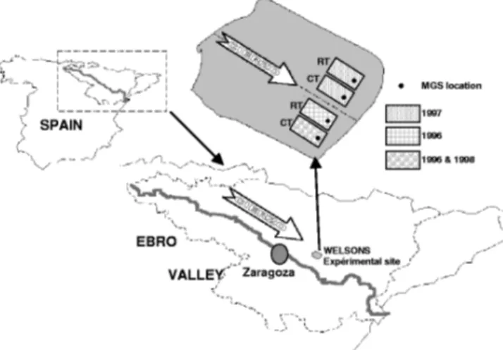
Fig. 1. General fetch of the WELSONS experimental site. One can notice the location of the conventional tillage (CT) and reduced tillage (RT) plots, changing according to years and the main wind direction following the Ebro Valley.
first present an investigation on the variance profile of the horizontal wind in the vicinity of the ground. The study has led to link this profile with some terrain characteristics, par-ticularly the friction velocity and the roughness length. Then, some studies regarding the influence of the terrain roughness on the horizontal wind integral scales are presented. Spatial correlation between the two stations is also examined. Fi-nally, the last part based on spectral analysis, reports some results related to the meteorological spectral gap, the spec-tral energy containing-scale, and the TKE dissipation rate.
2 Experiment
For a complete description of the WELSONS experiment, with a detailed description of the site, one should refer to Frangi and Richard (2000). The climate of this Spanish re-gion is strongly influenced by two winds, namely Cierzo and Borchono, which are bound to a specific orography. In fact, the channel formed by the Cantabrico Cordillera to the north-west, the Pyr´en´eees Mountains to the north and the Iberian Cordillera to the south of the Ebro River, funnels each air flow, resulting in the main wind directions of WNW and ESE. The Cierzo is the wind from the WNW direction, a very cold air stream in winter and cool in summer. Two main meteorological situations can explain its appearance. The first is an anticyclone over the Cantabrico Sea and a low-pressure system above the Mediterranean Sea; the second is a strong low-pressure system to the north of Europe, coupled with a high-pressure area over the Azores. The first situation generates dry (from the foehn effect, see Schneider, 1996), strong and continuous winds. Cierzo events with gusts over 30 m.s−1 are common in this region, especially during the summer (Biel and Garcia de Pedraza, 1962), and according to Skidmore (1965), erosive winds are those exceeding 5.3 m.s−1at 2 m height. In the second case, the air flow which
blows over the whole of Europe has strong oceanic charac-teristics and causes wet weather with heavy swell conditions on the Atlantic coastline. In the opposite direction the Bo-chorno blows, with an ESE main direction, which appears when a pressure gradient exists between the Mediterranean Sea and the Cantabrico Sea, with a low pressure field over the latter. The Bochorno is generally a light wind (except in stormy conditions), and its direction is less well defined; it is temperate and moist in winter, and dry in summer, with a Saharan influence.
The traditional farming system of cereal-follow rotation extends over 250 000 ha in Central Aragon (Lopez et al., 1996), and the soil during the fallow period is smooth and bare. The experimental field, located in an area called El Saso (41◦36′N, 0◦32′W, 285 m above mean sea level), 35 km away from Zaragoza in the Ebro Valley (Fig. 1), is ori-ented in the direction of the Cierzo prevailing wind (WNW). It remained untilled after a barley-fallow rotation. Fields sur-rounding it, in the upwind edge, had very sparse vegetation. On both sides, at a distance of about 200 m, there were wheat fields, with a vegetation canopy lower than 30 cm and fallow fields of stubble separated the wheat fields from the experi-mental plots. The soil was a silt with 19.3% of sand, 67.6% of silt and 13.1% of clay (Gerakis and Baer, 1999) in the first 20 cm. The experimental field was divided into two adjacent plots (130×160 m2) for the application of two tillage treat-ments with a 20 m separation distance: conventional tillage (CT) and reduced tillage (RT). The CT treatment consisted of mould-board ploughing, at a depth of 30–35 cm, followed by the pass of a compacting roller to obtain a very flat ground: it constitutes the traditional practice in this area. The RT treat-ment, an alternative practice of conservation tillage (Lopez et al., 1996), consists of a unique pass of a chisel plough at a depth of about 15–20 cm, yielding a ground with furrows. In both cases, the tillages were done in the WNW direction. So the soil was bare with very different surface conditions during the whole experiment.
Two micrometeorological ground station (MGS) systems (Frangi and Richard, 2000) have been developed and set up on the experimental field to study the dynamical characteris-tics of the soil surface and the energy budget partitioning on both plots. They were installed in the downwind edge of the field to avoid a fetch effect. The devices measure the energy budget parameters: wind speed and direction, air temperature and vapour pressure at two levels, net radiation and ground heat flux, soil and surface temperature, and atmospheric pres-sure. In addition, they record the wind profile every one sec-ond, through a set of 5 cup anemometers installed along a 4 m height vertical mast, in order to determine the roughness length and the friction velocity during wind erosion events (Frangi and Poullain, 1997). The five anemometer heights are 28, 53, 118, 203 and 402 cm. The two MGS are syn-chronized. The 1997 WELSONS experiment was conducted from 29 June to 25 September.
3 5 7 9 11 13
0:00 6:00 12:00 18:00 0:00
Daytime hours
M
e
an
w
in
d
velocit
y
(
m
/s
)
Level 1
Level 2
Level 3
Level 4
Level 5
Fig. 2. Variation of the mean wind ve-locity during the day of 25 July 1997 at different levels.
1.3 m), the variance reduction due to the inertial effects was estimated to range from 0.6 to 1.5%, respectively, for the top and bottom levels. In order to assess the magnitude of vari-ance losses deriving from an insufficient sampling frequency, a complementary study was carried out, in an urban area, at University D. Diderot (Paris 7), with a three-dimensional sonic anemometer (Campbell CSAT3). Thus, a variance drop of about 10% was found between samplings of 1 and 32 Hz, for wind velocity around 4 m.s−1, with turbulence intensity
of about 40%. In addition, the accordance found between the experimental and the von Karman spectra, notably in the up-per frequency part (see Sect. 3.3.2), reinforces credit to the quality of the data.
Data concerning the wind velocity fluctuations are system-atically detrended, except for the study of the spectral gap. In this case, the data corresponding to time intervals longer than 8 h are averaged over 2 or 3 s. The mean wind velocity at the highest level of plot CT is around 11 m.s−1during the day-time of 25 July 1997 and the turbulence intensity confined between 12% and 16% throughout the same day at the same level.
3 Results
3.1 Profile of the variance of the horizontal wind compo-nents in the ASL
The wind velocity variance, which represents the turbulent kinetic energy, is an important parameter of the ASL, since it conditions many phenomena taking place in this layer, such as the diffusion of chemical and physical aerosols, energy transfer between the mean and the turbulent flows, heat and mass transfer, extreme wind force exercised on structures, etc.
The wind data logged during the WELSONS experi-ment concern the bottom part of the ASL, since the lowest anemometer is located at 0.25 m from the ground, while the highest one is at 4 m (thus covering a height scale ratio of 16). This particularity of the experiment, due to its specific
objectives, is expected to produce somewhat different results from common micrometeorological experiments.
3.1.1 Variance of the horizontal wind components in the ASL
Despite the existence of long established relationships (Panofsky et al., 1977), the behaviour of the variance of the horizontal wind components in the ASL is still discussed, es-pecially the definition of their pertinent scaling parameters.
Thus, for Kaimal and Finnigan (1994), the horizontal wind components, contrary to the vertical one, are not governed by the Monin-Obukhov ASL similarity theory, which states that various atmospheric parameters and statistics, such as gra-dients, variances and co-variances, when normalized by ap-propriate powers of the scaling velocityU∗and the scaling temperatureθ∗, become universal functions of the stability parameter. This is because the wind horizontal components do not depend on the height throughout the surface layer and most of the ABL, even in highly unstable conditions (Gar-rat, 1992). This property could be explained by the influence of low-frequency eddies, either through boundary-layer in-stabilities or convection, which makes the ABL depth,Zh, the scaling height. Thus, in unstable conditions, Panofsky et al. (1977), proposed the following relationship:
σu U∗ ≈
σν U∗=
12−0.5Zi
L
1/3
, (1)
whereZi is the daytime ABL depth. The establishment of
this relationship relied on data obtained, on the one hand, from a mast up to 32 m and, on the other hand, from a teth-ered balloon for upper heights. Most of the data were ob-tained over water. No clear indications were available on the lowest measurement height, but a set of data from a 4-m height level is included.
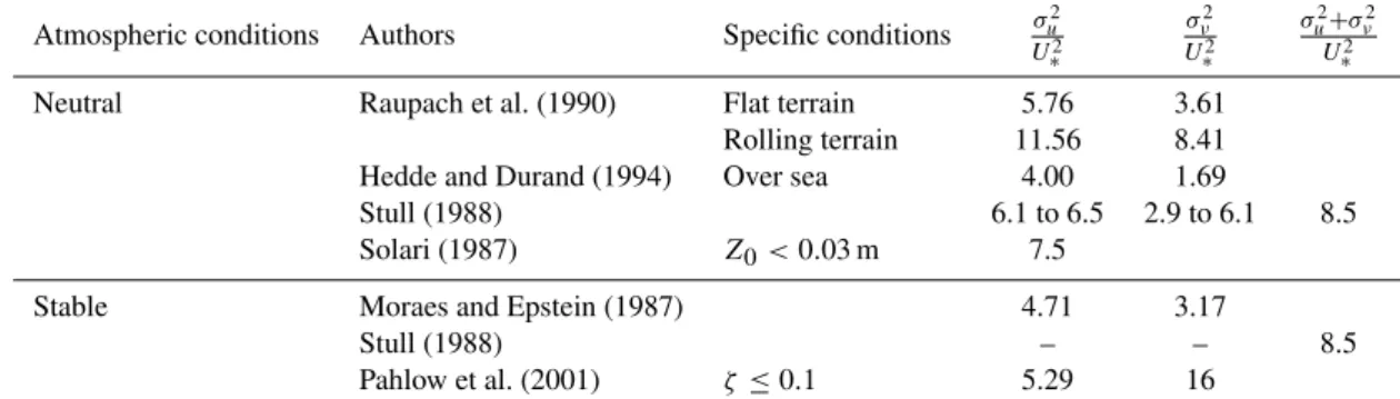
Table 1.Variances of the horizontal wind components in neutral and stable conditions in the ASL, according to authors
Atmospheric conditions Authors Specific conditions σ
2
u U2
∗
σν2 U2
∗
σu2+σν2 U2
∗
Neutral Raupach et al. (1990) Flat terrain 5.76 3.61
Rolling terrain 11.56 8.41
Hedde and Durand (1994) Over sea 4.00 1.69
Stull (1988) 6.1 to 6.5 2.9 to 6.1 8.5
Solari (1987) Z0<0.03 m 7.5
Stable Moraes and Epstein (1987) 4.71 3.17
Stull (1988) – – 8.5
Pahlow et al. (2001) ζ ≤0.1 5.29 16
-400 -320 -240 -160 -80 0 80 160 240 320 400
0:00 6:00 12:00 18:00 0:00
Daytime hours
M
o
ni
n-O
bukhov l
ength (m)
Fig. 3. Variation of the Monin-Obukhov length during the day of 25 July 1997 (Plot CT).
that the horizontal wind components followed the similarity theory yielding, for free convection:
σu U∗ =
σν U∗ =2.8
−z L
1/3
. (2)
Sa¨id (1988) and Id´e (1991) reported the same “1/3 law” with a constant of 2.0 and 5.4, respectively, instead of 2.8. Con-trary to the other studies, the latter was carried out over land, in the semiarid Sahel region of Africa.
In stable conditions, Pahlow et al. (2001), analysing data from a set of five experiments, distinguished between two cases according to the stability parameter. The five experi-ments were carried out in the ASL at heights ranging from 0.96 to 4.32 m. In weak stability conditions, i.e. when the stability parameterζ ≤ 0.1, they observed that the normal-ized horizontal wind components adopted a local z-less strat-ification behaviour, becoming thus constant (Table 1). When the stability parameter exceeds this value, they proposed the following equation:
σα
U∗ =a+b
z
L
c
, (3)
whereαrepresentsuandv;a,bandcequal 2.3, 4.3, and 0.5, respectively, for the longitudinal component, and 2.0, 4.0 and 0.6 for the transversal wind.
However, many authors indicate that, under stable condi-tions and in the ASL, the variances of horizontal wind com-ponents are constant. Table 1 summarises the typical val-ues encountered. The data of Moraes and Epstein (1987) are valid for heights up to 22.6 m, while no specific conditions were given by Stull (1988).
According to the Monin-Obukhov similarity theory, when conditions approach neutrality, the variances of the horizon-tal wind components become constant (Garrat, 1992). Typi-cal values of the constants are presented in Table 1. Thus, for the experimental data, the values are around 6 for common terrain. For rolling terrain, the variance increases up to 20 and decreases down to 6 over sea.
Solari (1987) proposed a relationship for turbulence in the near-neutral ASL in whichβu, the constant ratio between the
variance of the longitudinal wind velocityσu2and the square of the friction velocityU∗2, depends on the terrain roughness,
Z0, i.e.:
βu = σ
2
u U2
∗ =
7.5 for Z0≤0.03
4.5−0.856 ln(Z0)for 0.03≤Z0≤1
4.5 for Z0≥1,
(4)
whereZ0is expressed in meters.
Table 2.Linear regression parameters of the functionσ2/U∗2=f (ln(z))=aln(z)+b
R2>0.90 Slope,a Intercept,b −ln(Z0)
(total of cases = 475) average Variation Average Variation coefficient coefficient
Plot CT 95% 1.160 32% 8.074 15% 8.11
Plot RT 97% 1.156 26% 5.311 17% 5.81
2 4 6 8 10 12
1.0E-01 1.0E+00 1.0E+01
Height, z (m)
No
rmal
ised
vari
a
n
ce,
σσσσ
²/
U*
²
V= 7 m/s, 01:00 V= 8 m/s, 01:30 V= 9 m/s, 05:00 V=10 m/s, 15:00 V=11 m/s, 12:00
Fig. 4. Normalized variance (σu2/U∗2) as a function of the height logarithm, ln(z), for various wind velocity (7 to 11 m/s) and at different daytime (01:00 to 12:00 LT) (Plot RT, level 5, 25 July 1997).
vicinity of the ground. At these heights, the ground effects become important and thus, the roughness length becomes a relevant parameter, as it was in the case reported by Solari (1987). In addition, Hedde and Durand (1994) and Pahlow et al. (2001) reported that, in some circumstances, the variances of the horizontal wind components depend on the height. Be-sides any thermal stability considerations, the layer studied in the WELSONS experiment is rather a dynamic one, be-cause the considered heights are negligible compared to the Monin-Obukhov length (Fig. 3) and the friction velocity is high (respectively, 0.4 and 0.5 in the two plots). These con-ditions of the dynamic layer occurrence were specified by De Moor (1983).
3.1.2 Profile of the variance of the horizontal wind compo-nents in the WELSONS experiment
The wind velocity data stemming from cup anemometers are the sums of the horizontal wind components. Since the study does not include the vertical wind component, we decided to linearly detrend the turbulent wind fluctuations in order to re-move the mean flow influences. The variances are calculated over 14-min time intervals, to match with the data related to the friction velocity and the roughness length.
Figure 4 and Table 2 show that, in the specific experimen-tal conditions, the horizonexperimen-tal wind variance normalized by the square of the friction velocity is a linear function of the
logarithm of the height. In this analysis, the values of the friction velocity stem from previous published works (Frangi and Richard, 2000). In Table 2, we see that the linear correla-tion coefficientR2is higher than 0.9 in 95% of the 475 cases at plot CT and in 97% of the cases at plot RT. In light of this observation, it seems possible to model the normalized variance through the following relationship:
σ2 U2
∗
=aln(z)+b. (5)
Table 2 gives the values ofa andb. We notice that the values of the constant b (5.3 and 8.1, respectively, for the plots CT and RT), which represents the normalized variance at 1 m, are of the same magnitude as those reported in Ta-ble 1. We also observe that the mean values of the constanta
are roughly the same in the two plots, while the opposite of the logarithms of the roughness lengthsZ0are very close to
the corresponding values of the constantb(Table 2). This re-mark leads us to setb = −ln(Z0)and thus, the relationship
(5) becomes:
σ2 U2
∗
=aln(z)−ln(Z0). (6)
0.0 0.5 1.0 1.5 2.0 2.5 3.0 3.5
0.0 0.5 1.0 1.5 2.0 2.5 3.0 3.5
Modelling variance (m²/s²)
Exp
e
ri
men
tal
vari
a
n
ce (m²/
s²)
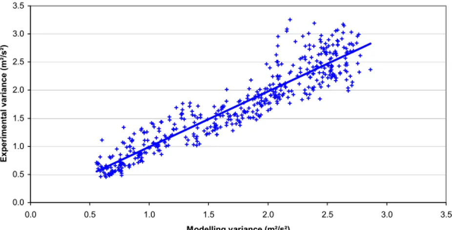
Fig. 5. Comparison between the ex-perimental and the modelled data of the variance (plot CT, level 5, 25 July 1997),y = 0.9871.x+0.0014, R2 = 0.8693.
Table 3. Parameters of the linear regression between the mod-elling and the experimental data of the variance according to the anemometer levels
Linear correlation Slope,a Intercept,b coefficient (R2)
Plot CT Level 1 0.90 0.97 0.06
Level 2 0.89 0.94 0.06
Level 3 0.87 0.95 0.04
Level 4 0.86 0.94 0.07
Level 5 0.87 0.99 0.00
Plot RT Level 1 0.88 1.15 0.03
Level 2 0.87 1.06 0.06
Level 3 0.86 1.06 0.10
Level 4 0.85 0.99 0.17
Level 5 0.84 0.88 0.08
coming from Eq. (6) to the experimental data. The fric-tion velocity and the roughness length values are provided by Richard (2000). Table 3 gives the regression parameters between the modelled and the experimental data. Thus, we notice that the determination coefficient, the slope and the vertical intercept indicate good agreement between the two data sets.
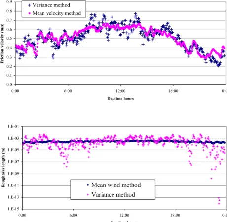
In addition, Eq. (6) offer a prospective opportunity for the determination of the friction velocity and the roughness length from the variance profile. Figures 6 and 7 compare the values of the friction velocity and roughness length stem-ming from the variance and the mean wind velocity methods. The correlation between the values of the friction velocity is 0.86 and 0.87, respectively, in plots CT and RT (for the 475 data of 25 July 1997, over 24 h). As far as the roughness length is concerned, which slightly varies, the correlation co-efficient is nearly meaningless.
3.2 Temporal and spatial autocorrelation of the horizontal wind
Correlation parameters, notably the correlation function, the time and length integral scales, and the decay factors, are important for the understanding of the structure of the wind flow in the ASL and consequently, for the modelling of other parameters such as the wind spectrum. Such parameters are also required in the assessment of forces deriving from wind gust for the stability of structures (Schettini and Solari, 1998; Toriumi et al., 2000). Through the five anemometer levels and the two plots, we investigate the temporal and spatial (horizontally) correlation functions and their relating param-eters, such as the time and length integral scales. As for the variance calculation, the wind velocity data are first linearly detrended within 15-min time interval samples.
The chart of the correlation function shows that, after a given time lag, the function begins oscillating within the value interval of[−0.2; +0.2]. This oscillation, which oc-curs after about ten seconds, can be explained as the influ-ence of less rapid varying eddies. This kind of influinflu-ence has been specified by Lumley and Panofsky (1964) in the calcu-lation of the velocity variance.
The time integral scale, which is given by the integral of the correlation function,ρ(t ), between 0 and∞, represents the time scale within which the considered turbulent parame-ter remains autocorrelated. For the experimental calculation of this scale, the correlation functionρ is approximated by the elementary function:
g(t )=b−aln(1+t ), (7)
wheretis the time (in second), andaandbare two constants. Althoughbis very close to 1, we did not fix it, in order to take into account the measurements’ uncertainty. For the experi-mental calculation of the time integral scale,g(t )offers two advantages compared to the well-known exponential equa-tion:
f (t )=exp
− t Tu
0.0 0.1 0.2 0.3 0.4 0.5 0.6 0.7 0.8 0.9
0:00 6:00 12:00 18:00 0:00
Daytime hours
F
ri
cti
on vel
o
ci
ty (m/
s)
Variance method
Mean velocity method
Fig. 6. Values of the friction veloci-ties. Comparison between the variance (cross) and the mean wind methods (dot), plot RT, 25 July 1997. The mean wind method data are from Richard (2000).
1.E-15 1.E-13 1.E-11 1.E-09 1.E-07 1.E-05 1.E-03 1.E-01
0:00 6:00 12:00 18:00 0:00
Daytime hours
Roughness l
ength (m)
Mean wind method Variance method
Fig. 7. Values of the roughness length. Comparison between the vari-ance (cross) and the mean wind meth-ods (dot), plot CT, 25 July 1997. The mean wind method data are from Richard (2000).
wheretis the time andTuis the time integral scale. On the
one hand,g(t )is expected to match with the first zero cross-ing value of the experimental correlation function and, on the other hand, it better correlates with the experimental data of the horizontal wind components. As suggested by Kaimal and Finningan (1994), the experimental computation of the time integral scale must take into account the first zero cross-ing value. This discussion does not mean that the theoretical exponential model of the correlation function is called into doubt.
Table 4 shows that the time integral scale is sensitive to the ground roughness and to the anemometer heights. In fact, it increases with the height and decreases with the roughness length. The ground vicinity, as well the terrain roughness, have, as particular effects, the disintegration of the eddies coherence.
The integral length scale,Lu, is obtained by multiplying the integral time scale by the mean wind velocity. This pa-rameter, also called the Eulerian length integral scale, is a measure of the average spatial extent or coherence of the fluctuations. Table 4 gathers the mean values of the length integral scale at the different heights and plots. The data are averaged between 07:00 LT and 17:00 LT, when the mean wind velocity varies slightly.
As the integral length scale values range from 28 to 90 m, no meaningful intercorrelation coefficient can be expected between the two stations distanced of 150 m. Thus, it was found that the correlation coefficient between the two plots,
ranges from−0.2 to 0.2, even for the upper anemometer lev-els (4 and 5).
3.3 Some spectral characteristics of the turbulent flow This section, which focuses on the spectral study of the tur-bulent flow, intends to show that the structure of the turtur-bulent flow is modified by the terrain roughness. In addition, it re-veals the spectral quality of the data measured by the cup anemometers.
3.3.1 The meteorological spectral gap and terrain rough-ness
The meteorological spectral gap is an important conceptual tool for the study of the turbulence. Application of the er-godic hypothesis principle leads to the estimation of the ad-equate averaging timeT, assuming an acceptable errorε, as follows (Lumley and Panofsky, 1964):
T = 2If ε2
f′2
f2 withε=
σf(T )
f , (9)
where f′2 is the ensemble variance of a stationary random
function f (t ) about its ensemble mean f, If is the time
integral scale andσf(T )is the ensemble standard over the
finite timeT.
Table 4.Ratio of the spectral energy-containing scale to the length integral scale and the Von Karman spectrum’s constantc, according to the plots and the anemometer levels. Average within the daytime interval 07:00–17:00 LT, 25 July 1997
Anemometer levels 1 2 3 4 5
Plot CT Mean time integral scale,Tu(s) 5.48 5.85 6.72 7.21 8.17 Time scale of the spectral peak,Tx(s) 24 29 40 43 48 Length scale of the spectral peak,Lx(m) 187 254 390 443 522 Length integral scale,Lu(m) 43.7 51.6 66.1 75.3 90.0
RatioLx/Lu 4.2 4.8 5.7 6.0 5.9
Constantc 2.59 2.92 3.50 3.65 3.61
Plot RT Mean time integral scale,Tu(s) 4.26 4.52 5.08 5.74 7.19 Time scale of the spectral peak,Tx(s) 14 17 28 35 42 Length scale of the spectral peak,Lx(m) 95 131 244 327 450 Length integral scale,Lu(m) 29.2 35.6 44.8 54.1 76.9
RatioLx/Lu 3.2 3.5 5.3 5.9 6.0
Constantc 1.97 2.17 3.27 3.60 3.65
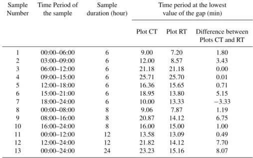
Table 5.Time period of the lowest value of the spectral gap according to the daytime period, the sample size and the experimental plot
Sample Time Period of Sample Time period at the lowest Number the sample duration (hour) value of the gap (min)
Plot CT Plot RT Difference between Plots CT and RT
1 00:00–06:00 6 9.00 7.20 1.80
2 03:00–09:00 6 12.00 8.57 3.43
3 06:00–12:00 6 21.18 21.18 0.00
4 09:00–15:00 6 25.71 25.70 0.01
5 12:00–18:00 6 16.36 15.65 0.71
6 15:00–21:00 6 18.95 13.80 5.15
7 18:00–24:00 6 10.00 13.33 −3.33
8 00:00–08:00 8 9.06 7.87 1.19
9 08:00–16:00 8 20.87 14.12 6.75
10 16:00–24:00 8 16.00 15.00 1.00
11 00:00–12:00 12 13.58 13.09 0.49
12 12:00–24:00 12 21.82 14.12 7.70
13 00:00–24:00 24 23.23 15.16 8.07
slowly varying one (mean flow), the average value over a finite time approaches the value of the slowly varying com-ponent, and the variance of the average goes through a mini-mum given by (Lumley and Panofsky, 1964):
σ2∼= 2I1 T f
2
1 +
T4
242f
′′2
2 , (10)
where the subscript 1 refers to the rapidly varying compo-nent and subscript 2 to the slowly varying one. The function
f2′′ is a second derivative of f2 andI1 is the time integral
scale. This relationship assumes thatT ≫I1and yet is small
enough to permit a local approximation off2by parabolic
arcs.
The optimum time that produces the minimum value ofσ2
can be obtained by differentiating Eq. (10), thus yielding:
T0= "
288I1
f12
f2′′2
#1/5
(11a)
and
σ02= 5I1 2T0
f12. (11a)
By combining these two equations, we obtain the follow-ing expression:
σ02= 5 2(288)1/5
10-1 100 101 102 103 0
0.02 0.04 0.06 0.08 0.1 0.12 0.14
F requency (h-1)
f.
S
(f)
/
σ
2
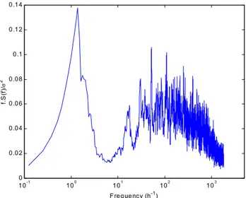
Fig. 8.Wind spectrum for the period 00:00–08:00 LT (Plot CT, 25 July 1997). One can see the spectral gap separating the mean and the turbulent flows.
Iff2 has a relatively sharp cutoff at the high-frequency
end, then f2′′2 will be roughly proportional to the fourth power of the cutoff frequency. Thus, the above variance be-comes proportional to the 4/5 power of the ratio of the inte-gral scale of the rapidly varying component to the smallest period of the slowly varying component.
The following investigation on the spectral gap uses the data obtained at 1-Hz frequency on the top anemometer lev-els (4 m) of the two experimental plots. Samples, ranging from 6 to 24 h time intervals, are constituted of the data of 25 July 1997 (see Table 5). The Fourier transform is applied on the wind fluctuations after removing the mean velocity. Data are not detrended, in order to conserve a meaningful part of the mean flow. For the samples of 12 and 24 h, the data have been, respectively, averaged over 2 and 3 s.
The charts of the above-mentioned data reveal a middle frequency zone where the spectral energy is much lower than the two separated parts of the curves (Fig. 8). This spectral gap, pointed out by Van der Hoven (1957), is one of the char-acteristics of the wind flow in the ASL. Its constitutes one of the theoretical basis of the turbulent study techniques, since it provides a way to separate the turbulent flow from the in-fluences of the mean flows (De Moor, 1983; Stull, 1988). In fact, the best method to separate the two scale flows consists of choosing the samples’ time intervalT, so that it falls into the gap zone. Thus, the spectral function of the “averaging operation” eliminates all the frequencies above 1/T, i.e. the turbulent frequencies.
In Table 5, we notice that the lowest amplitude of the spectral gap is located within the time period interval of 7 to 26 min, depending on the daytime period and the sample size. This is in accordance with the values indicated by Van der Hoven, who locates the centres of the spectral gap within the time period interval of 6 to 60 min.
10-3 10-2 10-1 100
10-1 100 101 102
frequency (Hz)
S
p
e
c
tra
l I
n
te
ns
it
y
, S
(f
) - (m
2.s -2)
Experim ental Spectrum Von Karm an Spectrum
Fig. 9.Comparison between the experimental and the Von Karman wind spectra (Plot CT, level 5, 25 July 1997, 02:45–03:00 LT).
By comparing the gap range frequencies over the two plots, we observe a shift of the gap zone towards the higher frequencies, from the plot CT to the plot RT, in 85% of the 13 studied samples. This shift is conserved in length scales, since the mean wind velocity is higher in plot CT than in plot RT. The roughness lengths of the two WELSONS exper-imental plots are about 0.3 and 3 mm (respectively, for plot CT and RT). Moreover, Eq. (12) shows that the time integral scale can have some influences on the characteristics of the spectral gap and that the time integral scale depends on the terrain roughness (See Sect. 3.2). So, we can conclude that the terrain roughness pushes the turbulent frequency range towards higher frequencies.
3.3.2 Some properties of the horizontal wind spectrum In this section we will validate the quality of the spectra stemming from the cup anemometer data and study the vari-ation of scales corresponding to the turbulent spectral peaks (energy-containing scales), in relation to the ground surface roughness and the anemometer levels. The spectra of the wind velocity fluctuations are computed from samples with a 15-min interval duration sampled at 1 Hz. Before apply-ing the Fourier transform, the data are first detrended. The study focuses on the time period 07:00–17:00 LT, which has stationary and high values of the mean wind velocity.
The obtained results are then compared with the Von Kar-man (1948) spectrum formula written as:
Su(f )=
4.σu2.Lu
U ·
"
1+
2.c.Lu U
2
·f2
#−5/6
, (13)
whereσuis the standard deviation of the horizontal wind,Lu
0 50 100 150 200 250
-70 -50 -30 -10 10 30 50 70
Stability parameter, z/L X 1,000
Nor
m
alis
ed T
K
E
dis
si
pation r
ate,
φ
ε
X 1,000
Daytime Night
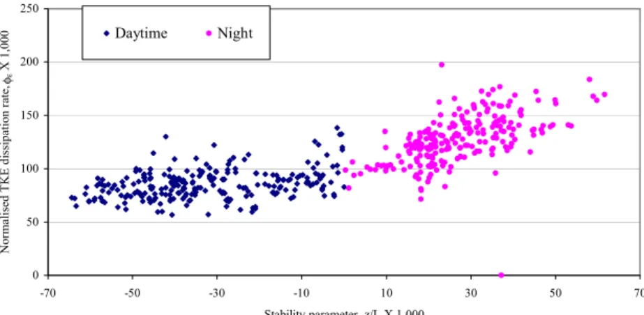
Fig. 10. Chart of the normalized TKE dissipation rate during daytime (diamond-shaped) and night (dot). Plot CT, level 5, 25 July 1997, through 24 h.
Figure 9 presents a comparison between the experimental and the modelled nightly spectrum of the horizontal wind. The results are similar, indeed even better during than the daytime when the mean wind is higher. Thus, we con-clude that the wind velocity fluctuation data furnished by the anemometers are good from a spectral point of view.
The chart in Fig. 9 uses log-log system axes. However, the spectra can also be charted in semilog axes, withf.Su(f )in
they-axis and ln(f )in thex-axis, which has the advantage of representing the energy of the corresponding frequency range by the area under the curve. In these axes, some characteris-tics regarding the spectral peak have been noticed. The time periodTx of the spectral peak (and subsequently the
corre-sponding length scale) increases with the anemometer height and decreases with the soil roughness (Table 4). The ratio of the time period between levels 1 and 5 is about 2 in plot CT and 4 in plot RT. This means that the rate also varies the roughness. This phenomenon of increasing length inte-gral scale with heights can be explained by the large eddies damping in the vicinity of the ground.
In addition, a relationship between the spectral peak length scale and the length integral scale is reported in literature. Thus, Kaimal and Finnigan (1994) pointed out that the spec-tral peak length scale,Lx, was roughly 6 times the integral length scale,Lu, i.e.:
Lx≈6.3Lu. (14)
This relationship can also be retrieved, for example, from the Von Karman spectrum model (see Eq. 14), by solving the equation:
d(f.Su(f ))
d (ln(f )) =0, (15)
leading to:
Lx Lu =c·
r
8
3 ≈1,63c, (16)
wherecis the above-mentioned constant of Eq. (13). In Table 4, we notice that the ratio of the spectral peak length scale to the length integral scale is roughly the same
as that reported by Kaimal and Finnigan (1994), for the two top levels (4 and 5). The constantcis of the same magnitude as that used in literature (3.60 versus 4.2). However, these parameters have to be adjusted for the lower levels (1 to 3). Thus, the length scales’ ratio range from 3.2 to 5, meanwhile the constantcvaries from 2 to 3. This suggests that the ratio, as well as the constantc, might depend on the height. 3.3.3 The behaviour of the kinetic energy dissipation rate The dissipation rate of the turbulent kinetic energy is one of the components of the turbulent kinetic energy budget and one of the important non-dimensional forms to emerge in the ASL (Kaimal and Finnigan, 1994). Its behaviour in the ASL is still discussed in despite of many long established mod-els. Its non-dimensional form,8ε, is assumed to follow the Monin-Obukhov similarity and thus, can be expressed as a function of the stability parameter,z/L, i.e.:
φε= k.z.ε
U3
∗
=fz L
, (17)
wherekandU∗are the Von Karman constant and the friction velocity, respectively.
Thus, Kaimal and Finnigan, relying essentially on the Kansas results (Businger et al., 1971; Wyngaard and Cot´e, 1971), re-examined and refined through comparison with other observations (Dyer, 1974; H¨ogstr¨om, 1988), proposed the following relationships:
φε=
(
1+0.5|Lz|2/33/2−2≤ Lz ≤0 1+5Lz 0≤ Lz ≤1.
(18)
We notice that, although it is not explicitly stated, these relationships are not valid beneath a certain height, otherwise the energy dissipation rateεwill tend to∞whenztends to 0. They also suggest that, in the nearly neutral conditions (i.e.
z/L≈0),8εis equal to 1, which means that the mechanical production term equals the dissipation one.
For stable conditions, the lower part of Eq. (18) can be rewritten as:
φε=A+γ z
1.E-03 1.E-02 1.E-01 1.E+00
1.E-05 1.E-04 1.E-03 1.E-02 1.E-01 1.E+00
Stability parameter, z/L
N
o
rmalis
ed TKE dis
si
pation rate,
φφφφεεεε
Level 1 Level 2 Level 3 Level 4 Level 5 Line 1 Line 2
Fig. 11. Chart of the normalized TKE dissipation rate by night for the five lev-els on plot CT (25 July 1997), i.e. level 1 (cross), level 2 (circle), level 3 (tri-angle), level 4 (X), level 5 (star), solid and dash lines verifying equationsy=
γ (z/L).
0 1 2 3 4 5 6 7 8
0:00 1:00 2:00 3:00 4:00 5:00 6:00
Daytime hours
Dissipation rate (X 1,
000,
m²/s
3)
Spectral method
Similarity method
Fig. 12. TKE dissipation rate. Com-parison between the similarity (cross) and the spectral (dot) methods. Plot CT, level 5, 25 July 1997.
In a recent paper, Pahlow et al. (2001) found that, in strong stability conditions, the function of the TKE dissipation rate was better described when the constantAequals 0.61, con-firming another result reported by Abertson et al. (1997). A summary of the experimental conditions of Pahlow et al. is already reported in Sect. 3.1.1. Furthering this result, Pahlow et al., relying on the behaviour of the heat flux in very strong stability, show that, for this limit,Abecomes very small com-pared toγ (z/L)and thus yielding:
φε =k.z.ε U3
∗ =γ z
L (20a)
and
k L ε U3
∗
=γ . (20b)
They reported a constantγ equal to 5. The same relation-ship was proposed by Stull (1988), for the stable ASL but withγ =3.7. In these conditions, the TKE dissipation rate obeys the concept of z-less stratification.
As underlined above, in the vicinity of the ground, Eq. (18) cannot describe the behaviour of the TKE dissipation rate. In these conditions, the z-less stratification law can be investi-gated. According to the similarity theory, the spectral density
of the wind velocity, in the inertial sub-rangeSu(k)is related to the kinetic energy dissipationεby the equation:
Su(κ)=αK ε2/3κ−5/3, (21)
whereκ is the wave number andαK the double of the
one-dimensional Kolmogorov constant taken to be 0.55, in accor-dance with Kaimal and Finningan (1994), who suggest the interval[0.5−0.6]. It appears thatεis a function of the ver-tical intercept of the regression line: ln(Su(κ))= f (ln(κ)).
Thus, we can calculate the dissipation rate by locating the in-ertial sub-range through the−5/3 slope of the log-log spec-trum chart.
Figure 10 shows the variation of the normalised TKE dis-sipation rate during 25 July 1997, at level 5 of Plot CT. One can see that the rate increases faster during the night than during the daytime with the stability parameter. By charting the values of the TKE dissipation rate, during night, for the five anemometer levels, we notice that all the data are con-centrated between two lines,D1andD2, verifying Eq. (20a),
(see Fig. 11). This observation leads us to express the TKE dissipation rate in the form of this equation.
stemming from Eq. (20b), by using the Monin-Obukhov length scale and the friction velocity determined by Richard (2000). Concerning the constantγ, the value 6 fits well in both plots CT and RT. This value is higher than that of 3.7 suggested by Stull (1988), but very to close the one reported by Pahlow et al. (2001), which is 5. The correlation coeffi-cient between the two data sets of the TKE dissipation rate is 0.79 in plot CT and 0.55 in plot RT.
This observation suggests that, in the vicinity of the ground, when the ground is colder than the air (a difference of about 2◦C in this case), the TKE dissipation rate can adopt the z-less stratification behaviour. Regarding the TKE dissi-pation rate under unstable conditions (during daytime), no clear specific behaviour has been noticed.
4 Conclusion
The behaviour of some ASL parameters in the close vicinity of the ground and according to the terrain roughness varia-tion was studied. Thus, this paper showed that the variance of the horizontal wind varies logarithmically with height. The parameters of the logarithmic function are closely related to the ASL parameters, particularly the friction velocity and the roughness length scale. These results could be used for accu-rate calculation of the wind velocity standard deviation and variance in models involving the two parameters, see Eq. (6). We also showed that the Eulerian integral scales were sensitive to the surface roughness and to the anemometer heights. In fact, the scale increases with the first parame-ter and decreases with the second one. Given the relation-ship between the time integral scale and the meteorological spectral gap (see Eq. 12), it was found that an increase in the roughness implied a shift towards higher frequencies in the location of the gap. In addition, the spectral peak length scale, which is linked to the Eulerian length integral scale (see Eq. 14), increases with height and decreases with the roughness.
The study of the TKE dissipation rate led to the conclusion that the parameter presents a z-less stratification behaviour under stable conditions. The results could be used, for ex-ample, to determine the magnitude of the heat flux from the friction velocity and the TKE dissipation rate, the latter being accessible from a single anemometer data.
We showed that cup anemometers could be used to study some turbulence characteristics in the ASL, in particular, in severe conditions of sand storms, where other sensors are less effective. Furthermore, specific characteristics could be revealed through data stemming from a cup anemometer. However, further studies are necessary to border the experi-mental limits of the apparatus.
Finally, the soil tillage treatment seemed to affect the tur-bulent flow characteristics of the ASL. Thus, the tillage mod-ifies the interface parameters between soil and atmosphere. This property could serve in many applications relating to soil erosion, agriculture, etc.
Abbreviations and acronyms
ABL Atmospheric Boundary Layer ASL Atmospheric Surface Layer CT Conventional Tillage ESE East-South-East
MGS Micrometeorological Ground Station
RT Reduced Tillage
TKE Turbulent kinetic energy
WELSONS Wind Erosion and Losses of Soil Nutrients in semiarid Spain
WNW West-North-West
List of Symbols
a Constant, generally slopes of linear regressions
A Constant
b Constant, generally the vertical intercept of linear regressions
c Constant
f frequency, random function, function
g function
If Time integral scale of the random functionf k Von Karman constant
L Monin-Obukhov length
Lu Length integral scale
Lx Spectral energy-containing scale Su Spectral density function ofu t time
T averaging time interval
Tu time integral scale u wind velocity
U mean wind velocity
U∗ Friction velocity z Height
Z0 roughness length
Zi daytime ABL depth αK Kolmogorov constant
βu Ratio between the variance ofuand the
square of the friction velocity
γ Constant
ε TKE dissipation rate, error
κ Wave number
σ standard deviation of the horizontal wind velocity
ζ Stability parameter
σα Standard deviation relating toα 8ε Normalized TKE dissipation rate
Acknowledgements. The European Commission-Environment and
Climate Programme DG XII, which sponsored this work under con-tract n◦ENV4-CT95-0182; Reviewers for their detailed inspection of the paper.
References
Albertson, J. D., Parlange, M. B., Kiely, G., and Eichinger, W. E.: The average dissipation rate of turbulent kinetic energy in the neutral and unstable atmospheric surface layer, J. Geophys. Res., 102, 13 423–13 432, 1997.
Biel, A. and Garcia de Pedraza, L.: El clima en Zaragoza y ensayo climatologico para el valle del Ebro, Ministerio del Aire, Servicio Meteorologico National, Publicaciones Ser. A (Memorias), 36, Madrid, 57 pp., 1962.
Businger, J. A., Wyngaard, J. C., Izumi, Y., and Bradley, E. F.: Flux profile relationships in the atmospheric surface layer, J. Atmos. Sci., 28, 181–189, 1971.
De Moor, G.: Les th´eories de la turbulence dans la couche limite atmosph´erique, Direction de la M´et´eorologie, 312 pp., 1983. Dyer, A. J.: A review of flux-profile relations, Bound. Layer
Mete-orol., 1, 363–372, 1974.
Frangi, J. P. and Poullain, P.: Un syst`eme d’acquisition haute vitesse de donn´ees dynamiques, associ´e `a une station de mesure du bilan d’´energie de surface, S´echeresse, 8, 70 p., 1997.
Frangi, J. P. and Richard, D. C.: The WELSONS experiment: overview and presentation of first results on the surface atmo-spheric boundary-layer in semiarid Spain, Ann. Geophysicae, 18, 365–384, 2000.
Fryrear, D. W. and Saleh, A.: Field wind erosion: vertical distribu-tion, Soil Sci., 155, 294–300, 1993.
Garrat, J. R.: The atmospheric Boundary Layer, Cambridge Atmo-spheric and Space Science Series, 316 pp., 1992.
Gerakis, A. and Baer, B.: A computer program for soil textural classification, Soil Sci. Soc. Am. J., 63, 807–808, 1999. Gillette, D. A., Blifford, I. H., and Fryrear, D. W.: The influence
of wind velocity on size distribution of aerosols generated by the wind erosion of soils, J. Geophys. Res., 79, 4068–4075, 1974. Hedde, T. and Durand, P.: Turbulence intensities and bulk
coeffi-cients in the surface layer above the sea, Bound.-Layer Meteo-rol., 71, 415–432, 1994.
H¨ogstr¨om, U.: Non-dimensional wind and temperature profiles. Bound.-Layer Meteor., 42, 55–78, 1988.
Id´e, H.: Dynamics and turbulence in the Sahelian surface atmo-spheric boundary layer (STARS experiment), in French, The-sis Nr 982, University Paul Sabatier, Toulouse, France, 228 pp., 1991.
Kaimal, J. C. and Finnigan, J. J.: Atmospheric Boundary Layer Flows, Their Structure and Measurement, Oxford University Press, 289 pp., Edition 1994.
Lopez, M. V., Arrue, J.-L., and Sanchez-Giron, V.: A comparison between seasonal changes in soil water storage and penetration resistance under conventional and conservation tillage systems in Aragon, Soil Tillage Res., 37, 251–271, 1996.
Lumley, J. L. and Panofsky, H. A.: The structure of atmospheric turbulence, Wiley-Interscience, New York, 239 pp., 1964. Lungu, D., Van Gelder, P. H. A. J. M., and Trandafir, R.:
Compara-tive study of Eurocode 1, ISO and ASCE procedures for calculat-ing wind loads, International Association for Bridge and Struc-tural Engineering (IABSE) Report. Vol. 74, pp. 345–354, Delft, March 1996.
Marticorena, B. and Bergametti, G.: Modeling the atmospheric dust cycle: 1. Design of a soil-derived dust emission scheme, J. Geo-phys. Res., 100, 16 415–16 430, 1995.
Monin, A. S. and Obukhov, A. M.: Basic laws of turbulent mixing in the ground layer of the atmosphere, Trans. Geophys. Inst. Akad. Nauk USSR, 151, 163–187, 1954.
Moraes, O. L. L. and Epstein, M.: The velocity spectra in the stable surface layer, Bound.-Layer Meteorol., 40, 407–414, 1987. Pahlow, M., Parlange, M. B., and Port´e-Agel, F.: On the
Monin-Obukhov similarity in the stable atmospheric boundary layer, Bound.-Layer Meteorol., 99, 225–248, 2001.
Panofsky, H. A., Tennnekes, H., Lenschow, D. H., and Wyngaard, J. C.: The characteristics of turbulent velocity components in the surface layer under convective conditions, Bound.-Layer Meteo-rol., 11, 355–361, 1977.
Quiroga, A. R., Buschiazzo, D. E., and Peinemann, N.: Manage-ment discriminant properties in semiarid soils, Soil Sci., 163, 591–597, 1998.
Raupach, M. R., Antonia, R. A., and Rajagopalan, S.: Rough-wall turbulent boundary layers, Appl. Mech. Rev., 44, 1–25, 1990. Richard, D. C.: Contribution to the study of the Spanish semi-arid
ASL, within the framework of WELSONS Project, in French, Thesis n◦2000PA077201, University Denis Diderot, Paris 7, France, 303 pp., 2000.
Sa¨ıd, F.: “Experimental study of the marine boundary layer: Turbu-lence structure and surface fluxes (TOSCANE-T Experiment)”, in French, Thesis Nr 248, University Paul Sabatier, Toulouse, France, 335 pp., 1988.
Schettini, E. and Solari, G.: Probabilistic modeling of maximum wind pressure on structures, J. Wind Eng. Ind. Aerodyn., 74–76, 1111–1121, 1998.
Schneider S. H.: Encyclopdia of climate and weather, Oxford Uni-versity Press (Pub), 929 pp., 1996.
Shiau, B.-S.: Velocity spectra and turbulence statistics at the north-eastern coast of Taiwan under high-wind conditions, J. Wind Eng. Ind. Aerodyn., 88, 139–151, 2000.
Skidmore E. L.: Assessing wind erosion forces: directions and rela-tive magnitudes, Soil Sci. Soc. Am. J. Proc., 29, 587–590, 1965. Solari, G.: Turbulence modelling for gust loading, J. Struct. Engin,
ASCE, 113, 7, 1150–1569, 1987.
Stull, R. B.: An Introduction to Boundary Layer Meteorology, At-mospheric Sciences Library, Kluwer Academic Publishers, 670 pp., 1988, Edition of 1999.
Toriumi, R., Katsuchi, H., and Furuya, N.: A study on spatial corre-lation of natural wind, J. Wind Eng. Ind. Aerodyn., 87, 203–216, 2000.
Van der Hoven, I.; Power Spectrum of Horizontal Wind Speed in the Frequency Range from 0.0007 to 900 Cycles per Hour, J. Meteor., 14, 160–164, 1957.
Von Karman, T.: Progress in the statistical theory of turbulence, Proc. Nat. Acad. Sci. 34, 530–539, 1948.
Wyngaard, J. C. and Cot´e, O. R.: The budgets of turbulent ki-netic energy and temperature variance in the atmospheric surface layer, J. Atmos. Sci., 28, 190–201, 1971.