Artificial Bee Colony with Different Mutation
Schemes: A comparative study
Iyad Abu Doush, Basima Hani F. Hasan, Mohammed Azmi Al-Betar, Eslam Al Maghayreh,
Faisal Alkhateeb, Mohammad Hamdan
Abstract
Artificial Bee Colony (ABC) is a swarm-based metaheuristic for continuous optimization. Recent work hybridized this algo-rithm with other metaheuristics in order to improve performance. The work in this paper, experimentally evaluates the use of differ-ent mutation operators with the ABC algorithm. The introduced operator is activated according to a determined probability called mutation rate (MR). The results on standard benchmark func-tion suggest that the use of this operator improves performance in terms of convergence speed and quality of final obtained solu-tion. It shows that Power and Polynomial mutations give best results. The fastest convergence was for the mutation rate value (MR=0.2).
Keywords: Artificial Bee Colony, Evolutionary Algorithms, Mutation, Meta-heuristic algorithm, Polynomial mutation.
1
Introduction
Meta-heuristic and evolutionary algorithms are computational meth-ods that solve a problem by iteratively trying to improve a candidate solution with regard to a given fitness function. While meta-heuristics do not guarantee reaching an optimal solution if one is available, they are useful for solving combinatorial optimization problems in both sci-ence and engineering. Many algorithms that mimic natural phenomena
c
such as genetic algorithms [21], simulated annealing [5], ant colony opti-mization [8], and particle swarm optiopti-mization [8] have shown significant efficiency in solving many real-world problems.
The Artificial Bee Colony (ABC) is an optimization algorithm based on the intelligent behavior of honey bees [1, 16]. In ABC, the position of a food source represents a possible solution to the optimization problem and the nectar amount of a food source corresponds to the quality (fitness) of the associated solution. In the ABC algorithm, the goal of the bees (employed bees, onlookers and scouts) is to discover the places of food sources with high nectar amount and finally the one with the highest nectar. The algorithm basically works as follows: employed bees go to their food source and return to hive. The employed bee whose food source has been abandoned becomes a scout and starts searching a new food source. Onlookers choose food sources depending on dances. Later on, the abandoned food sources are replaced with the new food sources discovered by scouts and the best food source found so far is registered. These steps are repeated until reaching the stop condition.
The ABC has been used to solve several optimization problems (e.g., forecasting stock markets [3, 18, 12], capacitated vehicle routing problem [29, 3, 9], multiproduct manufacturing system [2], and combat air vehicle path planning [13, 22, 30] ). Other researchers work on modifiying the original ABC (e.g., [4, 17]).
The remainder of this paper is organized as follows: Section 2 intro-duces the Artificial Bee Colony (ABC) Algorithm. Section 3 presents the different mutation methods. The experimental environment is pre-sented in Section 4. Finally, we conclude in Section 5.
2
The Artificial Bee Colony Algorithm
The Artificial Bee Colony (ABC) algorithm was first proposed by Karaboga in [14, 16]. In a real bees colony, there are different types of specialized bees performing different tasks. The main goal of the bees is to maximize the amount of nectar stored in the hive.
According to the ABC algorithm, the bees’ colony involves three different types of bees. Employed bees, onlooker bees and scouts. Half of the colony are employed bees and the reset are onlookers. Employed bees exploit food sources visited previously and provide the onlooker bees with information regarding the quality of the food sources they are exploiting. The onlooker bees use the information shared with em-ployed bees to decide where to go. Scout bees explore the environment randomly looking for new sources of food. When a food source ex-hausted, the corresponding employed bee becomes a scout. The main steps of the ABC algorithm are described below.
Step1: Initialize the food source positions.
In the ABC algorithm the position of a food source represents a pos-sible solution of the optimization problem and the amount of nectar at each food source represents the fitness of the corresponding solution. In this step of the algorithm, solutions xi (where i = 1. . . n) are ran-domly generated within the ranges of the problem’s parameters, where
n is the number of food sources (one source for each employed bee). Each solution is a vector ofddimensions, wheredis the number of the problem’s parameters.
The new food source (solution) is generated according to the fol-lowing formula:
yij =xij+ϕij(xij−xkj),
whereϕij is a random number in the range [-1,1],kis the index of the solution chosen randomly andj = 1, . . . , d.
After generating the new solution yi, the employed bee compares between it and the original solution xi and exploits the better one.
Step 3: Each onlooker bee chooses a food source based on its quality, generates a new food source and then exploits the best one.
An onlooker bee selects a food source based on the probability value associated with it. The probability value is calculated as follows:
pi =
F itnessi Pn
k=1F itnessk
,
whereF itnessi is the fitness of solution i, andnis the number of food sources which is equal to the number of employed bees.
Step 4: Stop the exploitation of the food sources exhausted and con-vert its employed bees into scouts.
A solution (represented by a food source) is said to be exhausted if it has not been improved after a predetermined number of execution cycles. The employed bee of each exhausted food source is converted into a scout that performs a random search for another solution (food source) based on the following formula:
xij =xminj + (xmaxj −xminj )∗rand,
wherexmaxj andxminj are the upper and the lower bounds of parameter (decision variable)j.
Step 5: Keep the best solution (food source) found so far.
3
Mutation Methods
The mutation method is an essential operator in EAs [7]. It normally provides a mechanism to explore unvisited regions in the search space. It operates with less consideration to the natural principle of the ‘sur-vival of the fittest’. Any successful EA should have a mutation mech-anism to ensure the diversification of the search space while makes use of the accumulative search.
Genetic Algorithm can be seen as the most popular EA algorithm that is widely used for optimization problems [25, 26]. It begins with population of individuals generated randomly. Evolutionary, it selects, recombines and mutates the current population to come up with a new population hopefully better. It exploits the current population using selection and recombination operators. It also explores the search space using mutation. This is necessary to prevent getting stuck in the local optima and increasing the chance of finding the global optima.
The way of diversifying the individuals in the population have been widely studied [11, 10, 7]. The mutation operator in GA randomly and structurally changes some genes in the individual without considering the characteristics of their parents. In order to implement a mutation operator, two issues should be watched: i) the probability of using mutation over population and ii) the power of mutation represented by the perturbation obtained in an individual.
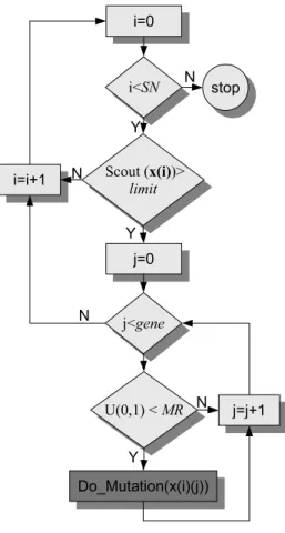
Similarly to GA, other population-based method have a mutation operator to diversify the search, e.g., the Random consideration in Harmony Search Algorithm, the scout bee in Artificial Bee Colony (ABC). Particularly in ABC, the scout bee provides a mechanism to diversify the individuals and therefore to prevent the search to fault down in a local optima trap.
Figure 1 flowcharts the scout bee process. At each iteration, all individuals,xi,∀i∈1. . . SN, in the population will be examined using
initialized by 0, otherwise it will be incremented by 1 until a certain limit exceeded, then aDo mutation() operator will be applied.
In general, the continuous optimization problem is formulated as follows
min{f(x)|x∈X},
where f(x) is the objective function; x={xi|i= 1, . . . , N} is the set
of decision variables (or genes). X={Xi|i= 1, . . . , N}is the possible
value range for each gene, whereXi ∈[Lx
i, Uxi], whereLxi andUxi are
the lower and upper bounds for the gene xi respectively and N is the number of genes.
In this paper, five mutation operators have been investigated in the scout bee operator. These mutation operators are controlled by a Mutation Rate (MR). The purpose of mutation is to diversify the search direction and to prevent the convergence into local optimum. Algorithm 1 shows that each gene in the selected individual will be examined for whether or not it will be changed randomly. In each mutation type, the change process is different as we will discuss below.
Algorithm 1 Scout Bee Procedure
1: fori= 1,· · · , SN do
2: if Scout[i]< limitthen
3: forj= 1,· · ·, N do
4: if U(0,1)< M R then
5: DO Mutation()
6: end if
7: end for
8: end if
9: end for
3.1 Original mutation
x′
i,j =Lxj+U(−1,1)(Uxj−Lxi).
In this type of mutation, the value of the gene is replaced randomly with a value within the range of decision variable [21] in the abandoned solutioni. Note thatU(−1,1) generates a random number between−1 and 1.
3.2 Non-uniform random mutation
The non-uniform random mutation is one of popular mutation types that is widely used in GA [21, 20]. In non-uniform mutation, as the generations increase, the step size decreases, therefore making a uni-form search in the initial stage of search and very little at later stages. In this type of mutation, the gene (xi,j) that met the probability of MR is changed as follows:
x′
i,j =xi,j×(1−U(0,1)( 1−t M SN)
b
),
where b is a system parameter determining the degree of dependency of iteration number (in this study, the value of b is fixed to 5 as rec-ommended by a previous study [21]), tis the generation (or iteration) number. And M SN refers to the maximum number of iterations in ABC. Note that the genex′
i,j is assigned with a value in a range [0, xi,j].
3.3 Makinen, Periaux and Toivanen (MPT) Mutation
Makinen, Periaux and Toivanen mutation, proposed by [19], is a rel-atively new mutation and has been applied to solve multidisciplinary shape optimization problem in addition to a large set of optimization problems with constrained nature. In this type of mutation, the gene (xi,j) that met the probability of MR is changed as follows:
x′
where
ˆ
tj ←
tj−(tj)×(tj−trj j )
b r
j< tj
tj rj= tj,
tj+ (1−tj)×( rj−tj
1−tj )
b r
j> tj
and
tj =
xi,j−Lxj Uxj−xi,j .
Normally, the value of b= 1.
3.4 Power Mutation
This type of mutation operator is based on power distribution, and proposed by [7]. It is an extended version of MPT mutation. In this type of mutation, the gene (xi,j) that met the probability of MR is changed as follows:
x′ i,j ←
½
xi,j−s×(xi,j−Lxj) t < r
xi,j−s×(Uxj−xi,j) otherwise,
where
t= xi,j−Lxj Uxj −xi,j ,
andsis a random number generated according to the final distribution, and r is a uniform random number generated in the range 0 and 1,
r∈[0,1].
3.5 Polynomial mutation
Polynomial mutation was first introduced by Deb and Agrawal in [6] which has been successfully applied for single and multi-objective op-timization problems. In this type of mutation, the gene (xi,j) that met the probability of MR is changed as follows:
x′
where
δq ← (
[(2r) + (1−2r) + (1−δ1)ηm+1]
1
ηm+1−1 r <0.5
1−[(2(1−r)) + (2(r−0.5)) + (1−δ2)ηm+1]
1
ηm+1 otherwise,
δ1 =
xi,j−Lxj Uxj−Lxj ,
δ2 =
Uxj−xi,j Uxj−Lxj .
Note that r is a uniform random number generated in the range 0 and 1,r∈[0,1].
3.6 Best-based Mutation
This type of mutation is initially proposed by [27]. It is effective and powerful mutation type for unconstrained large scaled optimization problems. In this type of mutation, four individuals are randomly selected (i.e., (xr1,xr2,xr3,xr4) from the entire population. After that,
the gene (xi,j) that met the probability of MR is changed as follows:
x′
i,j =xbest,j+F×(xr1,j−xr2,j) +F×(xr3,j−xr4,j),
wherexbest,j is the gene in the best individual from the entire popula-tion. F is an important parameter that ensures the balance between exploration and exploitation which normally is experimentally deter-mined, and takes a value range between 0 and 1.
4
Experimental results
were implemented with a multi-dimension (N=100), with the exception to Six-Hump Camel-Back function which is two-dimensional.
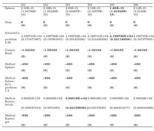
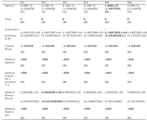
We conducted four different experiements, each one with different mutation rate (MR = 0, 0.2, 0.5, and 0.8). In each experiment we tested six different mutation methods: ABC original, Non-uniform, MPT, Power, Polynomial, and Best mutation. Each experiment was repeated 30 times with different random seeds. The average of the best values obtained by the algorithms is calculated. The obtained results of the mean best values and standard deviation are shown in tables 3, 4, 5, and 6.
The experiments were executed on a P4 machines with 1 GB of RAM using C++ under Microsoft Visual Studio environment. In all the experiments the values for common parameters are as follows: the population size (NP) was 100, the food sources was 50, the stopping criteria = 10,000, and the algorithm ran for 30 times. The limit is defined using the formula D* NP*0.5 which uses the dimension of the problem and the colony size to determine the limit value. These values are similar to what has been suggested in the state of the art methods. The results in tables 3, 4, 5, and 6 show that for the sphere function the mutation rate (MR=0.2) gives the best result, and the power mu-tation (M4) gives the best result. The best result for sphere function using other mutation rate values (MR= 0.5 and 0.8) was given by the polynomial mutation (M5).
On the other hand, for the Schwefel problem function the muta-tion rate (MR=0.2) gives the best result with MPT mutamuta-tion (M3). The shifted rosenbrock gives the best result using the mutation rate (MR=0.5) with MPT mutation (M3). The best result for shifted rosen-brock function using other mutation rate values (MR= 0.2 and 0.8) was given by the Non-uniform mutation (M2).
For the rest of the functions (i.e., step, camel-back, shifted sphere, shifted schwefel, and shifted rastrigin) all the mutation methods (M1-M6) with all mutation rates reached the global optimal solution.
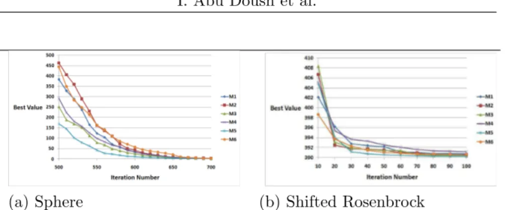
For the two functions polynomial mutation (M5) has the fastest con-vergence speed. The slowest concon-vergence speed for the sphere function was for Power mutation (M4). On the other hand, for the shifted rosenbrock, Best mutation (M6) has the slowest convergence speed.
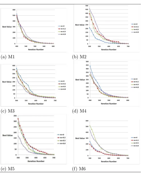
Figure 2 compares the effect of using different mutation rate val-ues on the convergence speed of the mutation method used (i.e., M1 to M6 in Table 1). Generally speaking the mutation rate (MR=0.2) has the fastest convergence speed for the mutation methods M1, M4, and M6 (Original ABC, Power, and Best). For the mutation meth-ods M3 and M5 (MPT and Polynomial), the mutation rate (MR=0.8) has the fastest convergence speed. These observations confirm the mean best results obtained, which are usually using mutation rate value (MR=0.2). This value allows diversifying the population without changing the population to be far from optimal solution.
Table 1. The different mutation schemes used in the experiments. Original ABC Non-uniform Makinen, Periaux and
Toivanen (MPT)
Power Polynomial Best
M1 M2 M3 M4 M5 M6
5
Conclusion and Further Work
cial Bee Colon y with Differen t Mutation Sc hemes Function Name Expression Search Range Optimum Value Category [24] Sphere func-tion [23]
f1(x) =
N
X
i=1
x2i xi ∈
[−100,100]
min(f1) =
f(0, . . . ,0) = 0
unimodal
Step function [23]
f2(x) =
N
X
i=1
(⌊xi+ 0.5⌋)2 xi ∈
[−100,100]
min(f2) =
f(0, . . . ,0) = 0
discontinuo-us unimodal
Schwefel’s problem 2.26 [31]
f3(x) =−
N
X
i=1
³
xisin (
q
|xi|)
´
xi ∈
[−500,500]
min(f3) =
f(420.9687, . . . ,
420.9687) =
−12569.5
difficult mul-timodal
Six-Hump Camel-Back function [23]
f4(x) = 4x21−2.1x41+ 1 3x
6
1+x1x2− 4x22+ 4x42
xi ∈
[−5,5]
min(f4) =
f(−0.08983,
0.7126)
low dimen-sional
I. Ab u Dou sh et al.
Name Range Value [24]
Shifted
Sphere func-tion [28]
f5(x) =
N
X
i=1
z2i + f bias1, where
z =x−o
xi ∈
[−100,100]
min(f5) =
f(o1, . . . , oN) = f bias1 =
−450 unimodal, shifted, sep-arable, and scalable Shifted Schwefel’s problem 1.2 [28]
f6(x) =
N X i=1 µ i X j=1 zj ¶2
+f bias2,
where z =x−o
xi ∈
[−100,100]
min(f6) =
f(o1, . . . , oN) = f bias6 =
−450 unimodal, shifted, non-separable, and scalable Shifted Rosenbrock [28]
f7(x) =
N−1
X
i=1
(100(zi+1−zi2)2+(zi −
1)2) +f bias
6, wherez =x−o
xi ∈
[−100,100]
min(f7) =
f(o1, . . . , oN) = f bias6 =
−390 multi-modal, shifted, non-separable, and scalable Shifted Rast-rigin [28]
f8(x) =
N
X
(z2i −10 cos (2πzi) + 10) +
xi ∈
[−5,5]
min(f8) =
f(o1, . . . , oN) = f bias9 =
multi-modal, shifted, sep-arable, and
Generally speaking the results show that Power and Polynomial mutations give best results. The mutation rate value (MR=0 and 0.8) gives the slowest convergence. On the other hand, the fastest conver-gence was for the mutation rate value (MR=0.2).
The future work can be experimenting different mutation schemes after modifying the original ABC algorithm to apply mutation on early stages of the algorithm. Currently, the algorithm uses mutation after exceeding the limit of reaching constant optimal solution. We could benefit more from the different mutation methods presented in this paper by applying them early in the ABC algorithm.
It might be interesting to adaptively select the mutation operator based on algorithm performance. But the algorithm needs to use a sin-gle best mutation rate, and mutation operator should be recommended, as it is not allowed to change this operator for each benchmark. For example, if the ABC algorithm is stuck in local optima, then use an-other operator in the hope to improve search capabilities and reach the global optima.
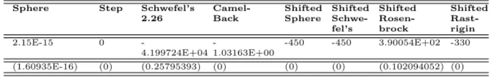
Table 3. Average and standard deviation (±SD) of the benchmark function results (N = 100), mr=0
Sphere Step Schwefel’s 2.26
Camel-Back
Shifted Sphere
Shifted Schwe-fel’s
Shifted Rosen-brock
Shifted Rast-rigin
2.15E-15 0
-4.199724E+04
-1.03163E+00
-450 -450 3.90054E+02 -330
(1.60935E-16) (0) (0.25795393) (0) (0) (0) (0.102094052) (0)
References
(a) M1 (b) M2
(c) M3 (d) M4
(e) M5 (f) M6
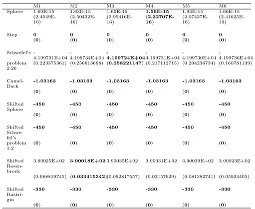
Table 4. Average and standard deviation (±SD) of the benchmark function results (N = 100), mr=0.2
M1 M2 M3 M4 M5 M6
Sphere 1.60E-15 1.63E-15 1.60E-15 1.56E-15 1.93E-15 1.66E-15 (2.4049E-16) (2.50432E-16) (2.95416E-16) (2.32707E-16) (2.07427E-16) (2.41625E-16)
Step 0 0 0 0 0 0
(0) (0) (0) (0) (0) (0)
Schwefel’s -4.199731E+04 -4.199734E+04 -4.199724E+04 -4.199731E+04 -4.199730E+04 -4.199736E+04 problem 2.26
(0.223375361) (0.256613668) (0.258221147) (0.217112715) (0.204236734) (0.160781139)
Camel-Back
-1.03163 -1.03163 -1.03163 -1.03163 -1.03163 -1.03163
(0) (0) (0) (0) (0) (0)
Shifted Sphere
-450 -450 -450 -450 -450 -450
(0) (0) (0) (0) (0) (0)
Shifted Schwe-fel’s
-450 -450 -450 -450 -450 -450
problem 1.2
(0) (0) (0) (0) (0) (0)
Shifted Rosen-brock
3.90025E+02 3.90018E+023.90035E+02 3.90031E+02 3.90039E+02 3.90023E+02
(0.088819745) (0.033415342)(0.092817557) (0.03157629) (0.081382741) (0.05924405)
Shifted Rastri-gin
-330 -330 -330 -330 -330 -330
(0) (0) (0) (0) (0) (0)
[2] S. Ajorlou, I. Shams, and M.G. Aryanezhad. Optimization of a multiproduct conwip-based manufacturing system using artificial bee colony approach. Proceedings of the International MultiCon-ference of Engineers and Computer Scientists, 2, 2011.
[3] B. Akay and D. Karaboga. Artificial bee colony algorithm for large-scale problems and engineering design optimization.Journal of Intelligent Manufacturing, pages 1–14, 2010.
oper-Table 5. Average and standard deviation (±SD) of the benchmark function results (N = 100), mr=0.5
M1 M2 M3 M4 M5 M6
Sphere 2.10E-15 2.16E-15 2.09E-15 2.13E-15 1.85E-15 2.14E-15 (1.84796E-16) (1.95236E-16) (2.65087E-16) (2.10979E-16) (1.61943E-16) (2.2148E-16)
Step 0 0 0 0 0 0
(0) (0) (0) (0) (0) (0)
Schwefel’s -4.199731E+04 -4.199736E+04 -4.199733E+04 -4.199731E+04 -4.199728E+04 -4.199735E+04 problem 2.26
(0.171671967) (0.195965045) (0.291429296) (0.214449308) (0.241189581) (0.247377045)
Camel-Back
-1.03163 -1.03163 -1.03163 -1.03163 -1.03163 -1.03163
(0) (0) (0) (0) (0) (0)
Shifted Sphere
-450 -450 -450 -450 -450 -450
(0) (0) (0) (0) (0) (0)
Shifted Schwe-fel’s
-450 -450 -450 -450 -450 -450
problem 1.2
(0) (0) (0) (0) (0) (0)
Shifted Rosen-brock
3.90025E+02 3.90036E+02 3.90016E+023.90019E+02 3.90039E+02 3.90032E+02
(0.056847244) (0.0972493) (0.031588391)(0.03157629) (0.066354577) (0.083040386)
Shifted Rastri-gin
-330 -330 -330 -330 -330 -330
(0) (0) (0) (0) (0) (0)
ators. Studies in Informatics and Control, 21(2):137–146, 2012. [5] Thomas Back. Evolutionary Algorithms in Theory and Practice.
OXFORD UNIVERSITY PRESS, New York, Oxford, 1996. [6] K. Deb and R. Agrawal. Simulated binary crossover for continuous
search space. Complex Systems, 9:115–148, 1995.
Table 6. Average and standard deviation (±SD) of the benchmark function results (N = 100), mr=0.8
M1 M2 M3 M4 M5 M6
Sphere 2.08E-15 2.10E-15 2.18E-15 2.16E-15 1.86E-15 2.09E-15 (2.32587E-16) (1.97095E-16) (1.55962E-16) (1.62883E-16) (1.65775E-16) (2.15497E-16)
Step 0 0 0 0 0 0
(0) (0) (0) (0) (0) (0)
Schwefel’s -4.199741E+04 -4.199729E+04 -4.199728E+04 -4.199734E+04 -4.199726E+04 -4.199728E+04 problem 2.26
(0.228840154) (0.165952493) (0.277530158) (0.158621939) (0.252550211) (0.175545128)
Camel-Back
-1.03163 -1.03163 -1.03163 -1.03163 -1.03163 -1.03163
(0) (0) (0) (0) (0) (0)
Shifted Sphere
-450 -450 -450 -450 -450 -450
(0) (0) (0) (0) (0) (0)
Shifted Schwe-fel’s
-450 -450 -450 -450 -450 -450
problem 1.2
(0) (0) (0) (0) (0) (0)
Shifted Rosen-brock
3.90034E+02 3.90020E+023.90031E+02 3.90042E+02 3.90027E+02 3.90061E+02
(0.074387028) (0.041508398)(0.05580612) (0.143667564) (0.06110496) (0.18150363)
Shifted Rastri-gin
-330 -330 -330 -330 -330 -330
(0) (0) (0) (0) (0) (0)
[8] Agoston E. Eiben and J. E. Smith. Introduction to Evolutionary Computing. SpringerVerlag, 2003.
[9] M. El-Abd. Black-box optimization benchmarking for noiseless function testbed using artificial bee colony algorithm. In Pro-ceedings of the 12th annual conference companion on Genetic and evolutionary computation, pages 1719–1724. ACM, 2010.
(a) Sphere (b) Shifted Rosenbrock
Figure 3. The convergence speed using different mutation methods (10,000 iterations and MR=0.8).
[11] F. Herrera and M. Lozano. Two-loop real coded genetic algorithms with adaptive control of mutation step sizes. Applied Intelligence, 13:187–204, 2002.
[12] T.J. Hsieh, H.F. Hsiao, and W.C. Yeh. Forecasting stock markets using wavelet transforms and recurrent neural networks: An in-tegrated system based on artificial bee colony algorithm. Applied Soft Computing, 11(2), 2010.
[13] F. Kang, J. Li, and Z. Ma. Rosenbrock artificial bee colony al-gorithm for accurate global optimization of numerical functions. Information Sciences, 2011.
[14] D. Karaboga and B. Akay. A comparative study of artificial bee colony algorithm. Applied Mathematics and Computation, 214(1):108–132, 2009.
[15] D. Karaboga and B. Basturk. Artificial bee colony (abc) opti-mization algorithm for solving constrained optiopti-mization problems. Foundations of Fuzzy Logic and Soft Computing, pages 789–798, 2007.
[17] Dervis Karaboga and Bahriye Akay. A modified artificial bee colony (abc) algorithm for constrained optimization problems. Ap-plied Soft Computing, 11(3):3021 – 3031, 2011.
[18] S. Kockanat, T. Koza, and N. Karaboga. Cancellation of noise on mitral valve doppler signal using iir filters designed with artificial bee colony algorithm. Current Opinion in Biotechnology, 22:S57– S57, 2011.
[19] Raino A.E. Makinen, Jacques Periaux, and Jari Toivanen. Multi-disciplinary shape optimization in aerodynamics and electromag-netics using genetic algorithms. International Journal for Numer-ical Methods in Fluids, 30(2):149–159, 1999.
[20] Z Michalewicz, T Logan, and S Swaminathan. Evolutionary op-erators for continuous convex parameter space. In Proceedings of Third Annual Conference on Evolutionary Programming. 1994. [21] Zbigniew Michalewicz. Genetic algorithms + data structures =
evolution programs (2nd, extended ed.). Springer-Verlag New York, Inc., New York, NY, USA, 1994.
[22] SN Omkar, J. Senthilnath, R. Khandelwal, G. Narayana Naik, and S. Gopalakrishnan. Artificial bee colony (abc) for multi-objective design optimization of composite structures. Applied Soft Com-puting, 2009.
[23] M. G. H. Omran and M. Mahdavi. Global-best harmony search. Applied Mathematics and Computation, 198(2):643–656, 2008. [24] Quan-Ke Pan, P.N. Suganthan, M. Fatih Tasgetiren, and J.J.
Liang. A self-adaptive global best harmony search algorithm for continuous optimization problems. Applied Mathematics and Computation, 216(3):830 – 848, 2010.
[26] W.M. Spears. Foundations of Genetic Algorithms. Morgan Kauf-mann, San Mateo, CA, 1993.
[27] Nadezda Stanarevic. Comparison of different mutation strategies applied to artificial bee colony algorithm. InProceedings of the 5th European conference on European computing conference, ECC’11, pages 257–262, Stevens Point, Wisconsin, USA, 2011. World Sci-entific and Engineering Academy and Society (WSEAS).
[28] P. N. Suganthan, N. Hansen, J. J. Liang, K. Deb, Y.-P. Chen, A. Auger, and S. Tiwari. Problem definitions and evaluation crite-ria for the cec 2005 special session on real-parameter optimization. Technical Report KanGAL Report#2005005, IIT Kanpur, India, Nanyang Technological University, Singapore, 2005.
[29] WY Szeto, Y. Wu, and S.C. Ho. An artificial bee colony algorithm for the capacitated vehicle routing problem. European Journal of Operational Research, 2011.
[30] C. Xu, H. Duan, and F. Liu. Chaotic artificial bee colony approach to uninhabited combat air vehicle (ucav) path planning.Aerospace Science and Technology, 2010.
[31] Xin Yao, Yong Liu, and Guangming Lin. Evolutionary program-ming made faster. IEEE Transactions on Evolutionary Computa-tion, 3(2):82 –102, 1999.
Iyad Abu Doush1, Basima Hani F. Hasan1, Received December 17, 2012 Mohammed Azmi Al-Betar2, Eslam Al Maghayreh1,
Faisal Alkhateeb1
1 Yarmouk University
Computer Science Department, Irbid, Jordan
Iyad Abu Doush
E–mail: iyad.doush@yu.edu.jo
2Jadara University