ISSN 0101-8205 / ISSN 1807-0302 (Online) www.scielo.br/cam
A filled function method for nonlinear systems
of equalities and inequalities
∗ZHONGPING WAN∗∗, LIUYANG YUAN and JIAWEI CHEN School of Mathematics and Statistics, Wuhan University
Wuhan, Hubei, 430072, P.R. China
E-mails: [email protected] / [email protected]
Abstract. In this paper a filled function method is suggested for solving nonlinear systems
of equalities and inequalities. Firstly, the original problem is reformulated into an equivalent
constrained global optimization problem. Subsequently, a new filled function with one parameter
is constructed based on the special characteristics of the reformulated optimization problem.
Some properties of the filled function are studied and discussed. Finally, an algorithm based
on the proposed filled function for solving nonlinear systems of equalities and inequalities is
presented. The objective function value can be reduced by half in each iteration of our filled
function algorithm. The implementation of the algorithm on several test problems is reported
with numerical results.
Mathematical subject classification: 65K05, 90C30.
Key words:nonlinear systems of equalities and inequalities, constrained global optimization,
filled function method.
1 Introduction
In this paper, we consider the following systems of nonlinear equalities and inequalities (for short, (SNEI)) defined by
(SNEI) ci(x)=0, i ∈ E, ci(x)≤0, i ∈ I, #CAM-410/11. Received: 10/IX/11. Accepted: 03/X/11.
where the functionsci : Rn → R are continuously differentiable, I ∪ E = {1, . . . ,m}andI ∩E = ∅. The systems of nonlinear equalities and inequalities have found myriad applications in various industrial and economic areas.
Ifn = m and I = ∅, the system (SNEI) reduces into a system of nonlinear equations, one classical problem in mathematics, for which there are many well-known methods, such as Newton-type methods, secant methods, and trust-region methods (see [3, 4, 5, 11] etc.). Similarly, in recent years these methods are also proposed to solve the system (SNEI) (see [6, 7, 15, 16, 17, 18, 19, 22, 26] etc.). A typical way of solving the system (SNEI) is to reformulate it into the fol-lowing constrained optimization problem (for short, (COP))
(COP)
f(x)=min
x∈Rn
1 2
P
i∈E
ci(x)2
,
s.t. ci(x)≤0,i ∈ I.
Some well-developed optimization methods are used to solve problem (COP). It is clear that global optimal solutions of problem (COP) with the zero objective function value correspond to the solutions of the system (SNEI). Therefore, efficient global optimization methods are crucial for successfully solving the system (SNEI).
[2, 12] and stochastic methods [20, 21]. Bai [1] proposed a filled function with three parameters for solving constrained nonlinear equations. However, in [1],
∇pr,c,q,x∗(x) = − 2c(x−x ∗
)
(kx−x∗k2+1)2 depends onx−x
∗, which is not desirable. Mo-tivated by these considerations, a novel filled function only with one parameter is constructed by employing the idea of penalty function in constrained opti-mization problem which is reformulated from the system (SNEI). Moreover, the gradient of the new filled function is not affected bykx −x∗k. The obtained nu-merical experiments show that the novel filled function method is of superiority over that in [1].
Outline. The rest of the paper is organized as follows. In section 2, a filled function is constructed for the reformulated constrained global optimization problem (COP). The corresponding filled function algorithm is presented in Section 3. Several numerical examples are reported in Section 4. and finally, some concluding remarks are made in section 5.
2 Filled function for problem (COP)
In this section, The following problem (COP) is considered
(COP) min
x∈Rn f(x)=
1 2
P
i∈E
ci(x)2
,
s.t.ci(x)≤0, i ∈ I.
Let
S = {x ∈ Rn|ci(x)≤0, i ∈ I},
S◦= {x ∈ Rn|ci(x) <0, i∈ I}.
Note thatS◦is not necessarily identical to the interior ofS.
Throughout the rest of the paper, we always assume that the following assump-tions for problem (COP) hold.
Assumption 2.1. I 6= ∅.
Assumption 2.3. S◦ 6= ∅ and cl S◦ = S, where cl A denotes the closure of set A.
By Assumption 2.3, we can see that for any x0 ∈ S, there exists a sequence
{xk} ⊂ S◦, such that limk→∞xk =x0.
It is easy to see that x∗ is a solution of the system (SNEI) if and only if it is a global minimizer of problem (COP) and satisfies that f(x∗)=0.
For a givenx∗∈ Swith f(x∗) >0, the definition of the filled function is given as follows.
Definition 2.4.A continuously differentiable function p(x,x∗)is called a filled function of problem (COP) at x∗ with f(x∗) > 0, if it satisfies the following conditions
(1) x∗is a strict local maximizer of p(x,x∗)on Rn;
(2) anyxˉ ∈ S\{x∗}with∇p(xˉ,x∗)=0implies f(xˉ) < f(2x∗); (3) any local minimizerx of pˉ (x,x∗)on Rnsatisfies f(xˉ) < f(x∗)
2 andxˉ ∈ S ◦;
(4) any local minimizerx of problem (COP) with fˉ (xˉ)≤ f(4x∗) andxˉ ∈S◦is a local minimizer of p(x,x∗)on Rn.
Remark 2.5. With the definition above, we know that if p(x,x∗) is a filled function of problem (COP) atx∗with f(x∗) >0, i.e. x∗is not a solution to the system (SNEI), any local minimizerxˉ of p(x,x∗)onRnsatisfies the inequality
f(xˉ) < f(2x∗) andxˉ ∈S◦.
In the following, a one-parameter filled function satisfying Definition 2.4 is introduced. To begin with, we design a continuously differentiable function Hr,a(t) with the following properties: it equals to a positive constanta when
t≥0, and it equals to 0 whent ≤ −r.
More specifically, for any given r > 0 anda > 0, we construct Hr,a(t) as
follows
Hr,a(t)=
a, t ≥0,
alog(1+r3)(−2(t+r)3+3r(t+r)2+1), −r <t<0,
0, t ≤ −r.
Note that the requirement for continuous differentiability ofHr,a(t)justifies the
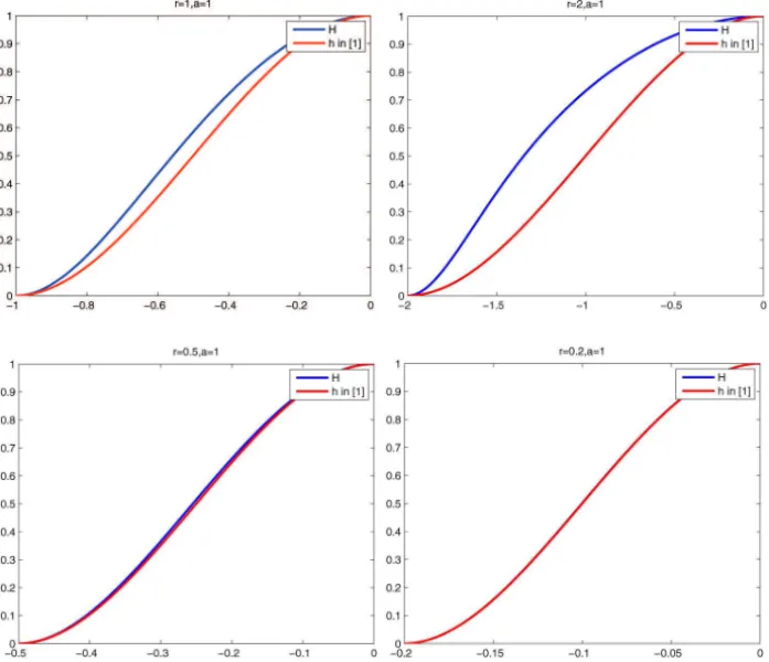
use of log function and cubic polynomial. The function Hr,a(t) differs from
hr,a(t)in [1], which we can get information from the figures below.
Figure 1 – The graphs of the functionsH andh.
From the figures above, it can be seen that when r ≥ 1, Hr,a(t) increases
faster thanhr,a(t)from−r to 0, while when 0<r <1, the function Hr,a(t)is
increasingly close tohr,a(t)asr is getting smaller and smaller.
It is not difficult to check that Hr,a(t) is continuously differentiable and
increasing onR. Obviously, we have
Hr′,a(t)=
0, t≥0,
−6a(t+r)2+6r a(t+r)
(−2(t+r)3+3r(t+r)2+1)ln(1+r3), −r <t<0,
0, t ≤ −r.
Given an x∗ ∈ S with f(x∗) > 0, the following filled function with one parameter is constructed
F(x,x∗,q)= −x−x∗
+q Hf(x∗)
4 ,1 ×Hf(x∗)
4 ,f(x∗)
f(x)− f(x
∗) 2
+X
i∈I
Hf(x∗) q ,f(x∗)
(ci(x))−
f(x∗)
2
(3)
where the only parameterq >0 andx∗is the current local minimizer of problem (COP). Clearly,F(x,x∗,q)is continuously differentiable on Rn.
Remark 2.6.Note thatF(x,x∗,q)includesP
i∈I Hf(x∗)
q ,f(x∗)
(ci(x))as a penalty
term to penalize unfeasible points.
The following theorems show that F(x,x∗,q)satisfies Definition 2.4 when the positive parameterq is sufficiently large.
Theorem 2.7. Let f(x∗) > 0, q > 0. Then x∗ is a strict local maximizer of F(x,x∗,q)on Rn.
Proof. Since x∗ is a local minimizer of f(x), there exists a neighborhood N(x∗, σ ) ofx∗ withσ > 0 such that f(x) ≥ f(x∗)for all x ∈ N(x∗, σ ) = {x| kx−x∗k < σ}. Then for any x ∈ N(x∗, σ ), x 6= x∗, q > 0, and 0 ≤
Hr,a(t)≤a, we have
F(x,x∗,q) <q =F(x∗,x∗,q).
Thus,x∗is a strict local maximizer of F(x,x∗,q)on Rn.
Theorem 2.7 reveals that the proposed new filled function satisfies condition (1) of Definition 2.4.
Theorem 2.8. Let f(x∗) > 0, q > 0. Then any point xˉ ∈ S\{x∗} with
∇F(xˉ,x∗,q)=0implies f(xˉ) < f(2x∗).
Proof. Assume that f(xˉ)≥ f(2x∗). Then for any pointxˉ ∈ S\{x∗}, we have
∇F(xˉ,x∗,q)= −(xˉ−x
∗)
k ˉx −x∗k 6=0.
which is a contradiction. Thus, any pointxˉ ∈ S\{x∗}with∇F(xˉ,x∗,q) = 0
Theorem 2.8 reveals that the proposed new filled function satisfies condition (2) of Definition 2.4.
Theorem 2.9.Let f(x∗) >0, q >0. Then any local minimizerx of Fˉ (x,x∗,q)
on Rnsatisfies f(xˉ) < f(2x∗) andxˉ ∈ S◦.
Proof. Letxˉ be a local minimizer ofF(x,x∗,q)on Rn, then∇F(xˉ,x∗,q)=
0 and xˉ 6= x∗ (since x∗ is a strict local maximizer of F(x,x∗,q) on Rn).
By contradiction, suppose that xˉ is neither a point satisfying f(xˉ) < f(2x∗)
norxˉ ∈ S◦. Then
∇F(xˉ,x∗,q)= −(xˉ−x
∗)
k ˉx −x∗k 6=0.
This is a contradiction. Therefore, ifxˉ is a local minimizer of F(x,x∗,q)on Rn, we have f(xˉ) < f(x∗)
2 and xˉ ∈S
◦.
Theorem 2.9 reveals that the proposed new filled function satisfies condition (3) of Definition 2.4.
Theorem 2.10.Let f(x∗) >0, q >0. Suppose that (SNEI) satisfies Assumption 2.2. Then there exists q0 >0such that when q ≥q0, any local minimizerx ofˉ
problem (COP) with f(xˉ)≤ f(4x∗)andxˉ ∈ S◦is a local minimizer of F(x,x∗,q)
on Rn. Furthermore, the number of pointxˆ ∈S◦with f(xˆ)≤ f(4x∗) is infinite. Proof. Let xˉ be a local minimizer of problem (COP) on S◦ with f(xˉ) ≤
f(x∗)
4 . Thenci(xˉ) < 0,i ∈ I and there exists a small enough number σ > 0 such that f(x) ≤ f(4x∗) and f(x) ≥ f(xˉ) for all x ∈ S ∩ N(xˉ, σ ), where N(xˉ, σ ) = {x ∈ Rn| kx− ˉxk < σ}. Thus, there exists q0 > 0 such that ci(xˉ) <−f(x
∗)
q0 ,i ∈ I. It follows that F(xˉ,x
∗,q)= − k ˉx−x∗kwhenq ≥ q0. Since F(x,x∗,q) ≥ − k ˉx −x∗k for any x ∈ Rn, xˉ is a global minimizer of F(x,x∗,q)on Rn. Therefore,xˉ is a local minimizer of F(x,x∗,q)on Rn. Let ˆ
x be a solution of (SNEI). Then we have thatxˆ 6= x∗. Bycl S◦=S, there exists a sequence{xk} ⊂ S such that xi 6= xj fori 6= j and lim
Theorems 2.10 show that, for allq ≥ q0, F(x,x∗,q)satisfies condition (4) of Definition 2.4. The following theorem shows that function F(x,x∗,q) has an interesting property.
Theorem 2.11. Let x1,x2∈S and the following conditions hold:
(i) min{f(x1),f(x2)} ≥ 12f(x∗); (ii) kx2−x∗k>kx1−x∗k.
Then, the inequality F(x1,x∗,q) > F(x2,x∗,q)holds for all q >0.
Proof. Since min{f(x1), f(x2)} ≥ 1 2f(x
∗), F(x
i,x∗,q)= − kxi−x∗k +q,
i=1,2. Therefore, for allq >0,F(x1,x∗,q) > F(x2,x∗,q)holds.
3 Filled function algorithm
In this section, a global optimization method for solving problem (COP) is presented based on the constructed filled function (3), which leads to a solu-tion or an approximate solusolu-tion to (SNEI).
Suppose that (SNEI) has at least one solution. The general idea of the global optimization method is as follows.
Let x0 ∈ S be a given initial point. Starting from this initial point, a local minimizerx0∗of problem (COP) is obtained with a local minimization method. The main task is to find deeper local minimizers of problem (COP) ifx0∗is not a global minimizer.
Consider the following filled function problem (for short, (FFP))
(FFP) min
x∈Rn F(x,x
∗
k,q).
whereF(x,xk∗,q)is given by (3).
Letxˉ0∗be a obtained local minimizer of problem (FFP) on Rn, then by
Theo-rem 2.9, we have f(xˉ0∗) < f(x
∗ 0)
2 andxˉ ∗
f(xˉ1∗) < f(x
∗ 0)
22 andxˉ1∗ ∈ S◦. Repeating this process, we can finally obtain a solution of the system (SNEI) or a sequence{ ˉxk∗} ⊂ S◦ with f(xˉk∗) < f(x
∗ 0)
2k ,
k = 1,2, . . .. For such a sequence { ˉxk∗}, k = 1,2, . . ., whenk is sufficiently large,xˉk∗can be regarded as an approximate solution of the system (SNEI).
Let x∗ ∈ S andǫ > 0, x∗ is called aǫ-approximate solution of the system (SNEI) ifx∗∈ Sand f(x∗)≤ǫ.
The corresponding filled function algorithm for the global optimization prob-lem (COP) is described as follows. The algorithm is referred as FFCOP (the filled function method for problem (COP)).
Algorithm FFCOP
Step 0: Choose small positive numbersǫ,λ, a large positive numberqU, and an
initial valueq0for the parametersq. (e.g. ǫ=10−8,λ=10−5,qU =105 andq0 = 100). Choose a positive integer numberK (e.g. K =2n) and directions ei, i = 1, . . . ,K, are the coordinate directions. Choose an
initial pointx0∈S. Setk :=0.
If f(x0)≤ ǫ, then let xk∗ := x0and go to Step 6; otherwise, let q := q0 and go to Step 1.
Step 1: Find a local minimizerxk∗of the problem (COP) by local search methods starting fromxk. If f(xk∗)≤ǫ, go to Step 6.
Step 2: Let
F(x,xk∗,q)= −x −xk∗
+q Hf(x∗k)
4 ,1 ×Hf(x∗
k) 4 ,f(xk∗)
f(x)− f(x
∗
k)
2
+X
i∈I
Hf(x∗ k) q ,f(xk∗)
(ci(x))−
f(xk∗)
2
(4)
whereHr,a(t)is defined by (1). Set l=1 and u=1.
Step 3: (a) Ifl> K, setq :=10q, go to Step 5; otherwise, go to (b).
(b) If u ≥ λ, set ykl := xk∗+uel, go to (c); otherwise, setl := l+1,
u=1, go to (a).
(c) If ylk ∈S, go to (d); otherwise, setu:= u
(d) If f(ykl) < f(x
∗ k)
2 , then set xk+1 := y
l
k, k := k +1, go to Step 1;
otherwise, go to Step 4.
Step 4: Search for a local minimizer of the following filled function problem starting fromyl
k
min
x∈Rn F(x,x
∗
k,q). (5)
Once a point yk∗ ∈ S◦with f(yk∗) < f(x
∗ k)
2 is obtained in the process of searching, setxk+1:= yk∗,k:=k+1 and go to Step 1; otherwise continue
the process. Let xˉk∗ be an obtained local minimizer of problem (5). If
ˉ
xk∗satisfies f(xˉk∗) < f(x
∗ k)
2 andxˉ ∗
k ∈ S◦, then setxk+1 := ˉxk∗,k :=k+1
and go to Step 1; otherwise, setu:= 10u, and go to Step (3b). Step 5: Ifq ≤qU, go to Step 2.
Step 6: Letxs =xk∗and stop.
From Theorems 2.7-2.10, it can be seen that ifλis small enough,qU is large enough, and the direction set{e1, . . . ,eK}is large enough,xs can be obtained
from Algorithm FFCOP within finite steps.
4 Numerical experiment
In this section, several sets of numerical experiments are presented to illustrate the efficiency of Algorithm FFCOP. All the numerical experiments are imple-mented in Matlab2010b. In our programs, the local minimizers of problem (FFP) and problem (COP) are respectively obtained by the Quasi-Newton method and the SQP method. k∇f(x)k ≤10−8is used as the terminate condition.
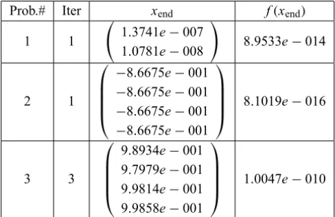
The data of the problems is shown in Table 1. The number of the problem is shown in column 1, the source of the problem in column 2 and the number of the set of equalities(mE), the set of inequalities(mI)and variables (n)in the
last column.
Initial points are the same as in the cited references.
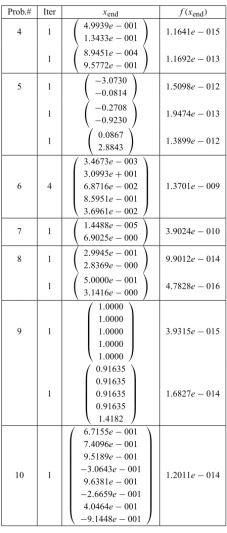
The number of problems (column 1), the number of iterations (Iter, column 2), the approximation solution to (SNEI) (xend, column 4) and the final functional
The first three problems are nonlinear inequalities, Problem 4 is square in-equalities and the last six problems are linear inin-equalities. From Table 2-3, it can be seen that the number of iterations of problem 1, 2, 3 is respectively 1, 1, 3, while the number of iterations of the same problems are 4, 11, 8 in [1]. More-over, from Table 4, it can be see that our filled function method is also effective to solve those problems which have square inequalities and linear inequalities.
Prob.# Test problem, source mE mI n
1 Problem 32 in [23] 2 2 2
2 Problem 93 in [23] 4 2 4
3 Problem 128 in [23] 4 2 4
4 Problem 5.1 in [22] 1 2 2
5 Test 14.1.1 in [8] 2 4 4
6 Test 14.1.2 in [8] 5 10 5
7 Test 14.1.3 in [8] 2 4 2
8 Test 14.1.4 in [8] 2 4 2
9 Test 14.1.5 in [8] 5 10 5
10 Test 14.1.6 in [8] 8 16 8
Table 1 – Data of the problems.
Prob.# Iter xend f(xend)
1 1 1.3741e−007
1.0781e−008
!
8.9533e−014
2 1
−8.6675e−001 −8.6675e−001 −8.6675e−001 −8.6675e−001
8.1019e−016
3 3
9.8934e−001 9.7979e−001 9.9814e−001 9.9858e−001
1.0047e−010
Prob.# Iter xend f(xend)
1 4 5.5533e−007
−3.0155e−006
!
1.0915e−011
2 11
−8.6675e−001 −8.6674e−001 −8.6675e−001 −8.6674e−001
1.0448e−012
3 8
−3.1394e−002 0.1660 −3.1269e−002
0.1843
2.5058e−009
Table 3 – Numerical results of Algorithm 3.1 in [1].
5 Conclusions
In this paper, the filled functionF(x,x∗,q)with one parameter is constructed for solving nonlinear systems of equalities and inequalities and it has been proved that it satisfies the basic characteristics of the filled function definition. Promising computation results have been observed from our numerical experiments. In the future, the filled function method can be used to solve other problems such as nonlinear feasibility problems with expensive functions and so on.
Acknowledgments. We are greatly indebted to the anonymous referees and Professor J.M. Martínez as the Editor of our paper for their very careful and valuable comments that helped improve this manuscript.
REFERENCES
[1] F.S. Bai, M. Mammadov, Z.Y. Wu and Y.J. Yang, A filled function method for constrained nonlinear equations. Pac. J. Optim.,4(2008), 9–18.
[2] J. Barhen, V. Protopopescu and D. Reister, TRUST: A deterministic algorithm for global optimization. Science,276(1997), 1094–1097.
[3] A.R. Conn, N.I.M. Gould and P.L. Toint,Trust region methods. SIAM, Philadel-phia, USA (2000).
[4] J.W. Daniel, Newton’s method for nonlinear inequalities. Numer. Math., 21
Prob.# Iter xend f(xend)
4 1 4.9939e−001 1.3433e−001
!
1.1641e−015
1 8.9451e−004 9.5772e−001
!
1.1692e−013
5 1 −3.0730
−0.0814 !
1.5098e−012
1 −0.2708
−0.9230 !
1.9474e−013
1 0.0867
2.8843 !
1.3899e−012
6 4
3.4673e−003 3.0993e+001 6.8716e−002 8.5951e−001 3.6961e−002
1.3701e−009
7 1 1.4488e−005 6.9025e−000
!
3.9024e−010
8 1 2.9945e−001 2.8369e−000
!
9.9012e−014
1 5.0000e−001 3.1416e−000
!
4.7828e−016
9 1
1.0000 1.0000 1.0000 1.0000 1.0000
3.9315e−015
1
0.91635 0.91635 0.91635 0.91635 1.4182
1.6827e−014
10 1
6.7155e−001 7.4096e−001 9.5189e−001
−3.0643e−001 9.6381e−001
−2.6659e−001 4.0464e−001
−9.1448e−001
1.2011e−014
[5] J.E. Dennis and R.B. Schnabel, Numerical methods for unconstrained optimiza-tion and nonlinear equaoptimiza-tions. SIAM, Philadelphia, USA (1996).
[6] J.E. Dennis Jr., M. EL-Alem and K. Williamson,A trust-region approach to non-linear systems of equalities and inequalities. SIAM J. Optim.,9(1999), 291–315. [7] I.I. Dikin, Solution of systems of equalities and inequalities by the method of
interior points. Cybernetics and Systems Analysis,40(2004), 625–628.
[8] C.A. Floudas et al., Handbook of Test Problems in Local and Global Optimiza-tion, Nonconvex Optimization and its Applications. Kluwer Academic Publishers, Dordrecht,33(1999).
[9] R.P. Ge, A filled function method for finding a global minimizer of a function of several variables. Math. Program.,46(1990), 191–204.
[10] R.P. Ge and Y.F. Qin, A class of filled functions for finding global minimizers of a function of several variables. J. Optim. Theory. Appl.,54(1987), 241–252. [11] C.T. Kelley, Iterative methods for linear and nonlinear equations. SIAM,
Philadelphia, USA (1995).
[12] A.V. Levy and A. Montalvo,The tunneling algorithm for the global minimization of function. SIAM J. Sci. Stat. Comput.,6(1995), 15–27.
[13] Y. Lin, Y.J. Yang and M. Mammadov,A new filled function method for nonlinear equations. Appl. Math. Comput.,210(2009), 411–421.
[14] Y. Lin and Y. Yang, Filled function method for nonlinear equations. J. Comput. Appl. Math.,234(2010), 695–702.
[15] M. Macconi, B. Morini and M. Porcelli,Trust-region quadratic methods for non-linear systems of mixed equalities and inequalities. Appl. Numer. Math.,59(2009), 859–876.
[16] B. Morini and M. Porcelli, TRESNEI, A Matlab trust-region solver for sys-tems of nonlinear equalities and inequalities. Comput. Optim. Appl., (2010), doi: 10.1007/s10589-010-9327-5.pdf.
[17] U.M. Garcia-Palomares, A global quadratic algorithm for solving a system of mixed equalities and inequalities. Math. Program.,21(1981), 290–300.
[18] B.T. Polyak, Gradient methods for solving equations and inequalities. USSR Comput. Math.,4(1964), 17–32.
[20] A.H.G. Rinnoy Kan and G.T. Timmer, Stochastic global optimization methods, part I:clustering methods. Math. Program.,39(1987), 27–56.
[21] A.H.G. Rinnoy Kan and G.T. Timmer, Stochastic global optimization methods, part II: multi-level methods. Math. Program.,39(1987), 57–78.
[22] S.M. Robinson,Extension of Newton’s method to nonlinear functions with values in a cone. Numer. Math.,19(1972), 341–347.
[23] D. Bini and B. Mourrain,Polynomial test suite.The website http://www-sop.inria.fr/saga/POL/.
[24] Z.Y. Wu, M. Mammadov, F.S. Bai and Y.J. Yang, A filled function method for nonlinear equations. Appl. Math. Comput.,189(2007), 1196–1204.
[25] Z.Y. Wu, F.S. Bai, H.W.J. Lee and Y.J. Yang, A filled function method for con-strained global optimization. J. Glob. Optim., (2007), doi: 10.1007/s10898-007-9152-2.
[26] L. Yang, Y.P. Chen and X.J. Tong,Smoothing newton-like method for the solution of nonlinear systems of equalities and inequalities. Numer. Math. Theor. Meth. Appl.,2(2009), 224–236.
![Table 3 – Numerical results of Algorithm 3.1 in [1].](https://thumb-eu.123doks.com/thumbv2/123dok_br/18978285.456092/12.918.216.705.131.448/table-numerical-results-algorithm.webp)