ESTIMATING SEA ICE PARAMETERS FROM MULTI-LOOK SAR IMAGES USING
FIRST- AND SECOND-ORDER VARIOGRAMS
Xiaojian Wang a, Yu Li a, Quanhua Zhao a, *
a
Institute of Remote Sensing Science and Application, School of Geomatics, Liaoning Technical University, Fuxin Liaoning, 123000 - [email protected]
Commission II, WG II/4
KEY WORDS: SAR imagery, Spatial structure of sea ice, Multi-Gamma model, Mosaic model, Variogram
ABSTRACT:
The spatial structures revealed in SAR intensity imagery provide essential information characterizing the natural variation processes of sea ice. This paper proposes a new method to extract the spatial structures of sea ice based on two spatial stochastic models. One is a multi-Gamma model, which characterizes continuous variations corresponding to ice-free area or the background. The other is a Poisson line mosaic model, which characterizes the regional variations of sea ice with different types. The linear combination of the two models builds the mixture model to represent spatial structures of sea ice within SAR intensity imagery. To estimate different sea ice parameters, such as its concentration, scale etc. We define two kinds of geostatistic metrics, theoretical first- and second-order variograms. Their experimental alternatives can be calculated from the SAR intensity imagery directly, then the parameters of the mixture model are estimated through fitting the theoretical variograms to the experimental ones, and by comparing the estimated parameters to the egg code, it is verified that the estimated parameters can indicate sea ice structure information showing in the egg code. The proposed method is applied to simulated images and Radarsat-1 images. The results of the experiments show that the proposed method can estimate the sea ice concentration and floe size accurately and stably within SAR testing images.
* Corresponding author
1. INTRODUCTION
Sea ice plays a very important role on hydrology, atmospheric thermal cycle, ocean currents and ecosystem in high latitudes, especially the Polar Regions (Zhu et al., 2012; Emilio et al., 2010). Sea ice limits shipping in high latitudes and requires special attentions when planning and running offshore activities in the Arctic Ocean and its peripheral seas (Johannessen et al., 2007). Consequently, timely obtaining the information of sea ice in a wide range is becoming more and more urgent for many governments and organizations. With the development of aerospace and aviation technology, remote sensing has proved to be a powerful tool for monitoring sea ice. Compared with the optical remote sensing, synthetic aperture radar (SAR) systems have been shown to be very useful due to its capability of acquiring data under all weather condition, during day and night, and are widely applied to marine , forestry, environment, agriculture fields (Kerman, 1999).
Estimating parameters of sea ice such as its concentration, size, age from SAR imagery is always a difficult task. Currently, many methods have been proposed to extract sea ice information. Nystuen and Garcia (1992) used both texture and standard statistics to classify sea ice types, where both of them are derived from a grey-level co-occurrence metrics (GLCM). In their experiments, they found that in some special ice zone, because of the movement of sea ice, a kind of new ice, called “odden” and multiyear ice, are of a SAR backscatter property and difficult to be distinguished. Soh and Tsatsoulis (1999) used GLCM to quantitatively evaluate textural parameters and determined the optimal parameters and representations for mapping sea ice texture. They investigated the quantization, displacement and orientation factors of GLCM on SAR sea ice imagery. They concluded that matrices with a range of displacement values are more adequately representative of a
texture than a single χ2-optimal matrix. Because of the movement of ocean currents and winds, different types of sea ice may have the same backscatter and vice verse. These phenomena will lead to incorrect classification of sea ice. Some researchers (Clausi & Deng, 2004; Ochilov & Clausi, 2012) investigated operational segmentation and classification methods by comparing three kinds of texture feature extraction methods and four types of segmentation models. After that, different extraction methods are combined with different segmentation models to do experiments. The gamma mixture model followed by a MRF label model is able to demarcate ice from open water region. All above studies used the traditional statistical metrics and considered the autocorrelation of sea ice only. Although the ice age is derived only from texture structure, it is not so accurate, and there is so much unknown information about sea ice. This paper considers both the autocorrelation of sea ice and the correlation between sea ice and the open water. Spatial statistical metrics are used to estimate the basic parameters of sea ice, such as total concentration and floe size of sea ice.
According to the properties of SAR imagery and sea ice spatial structure, we build two stochastic models, one is multi-Gamma model and the other is Poisson mosaic model. Then two kinds of geostatistic metrics are used to measure the spatial structure of sea ice. Theoretical variograms are built based on the two stochastic models, and the experimental variograms are calculated from the images. Then fit the theoretical variograms to the experimental variograms and the parameters are estimated in the theoretical variograms.
a summary of findings and suggestions for future enhancements in Section 4.
2. MODELS AND VARIOGRAMS 2.1 Random function and variogram
From spatial statistics point of view, the spatial structure and variability revealed in SAR data can be modeled by a regionalized variable z(x), which is simply considered as the realization of a random function Z(x) constructed at all points x of a given region D ⊂ R2, while Z={Z(x) : x ∈ D ⊂ R2} defines a random field on D.
The SAR data have been translated into general datum for analyzing. A stationarity condition should be set up first. Let
Z(x) be the second-order stationarity random function, then it is of the following properties,
E Z⎡⎣ (x)⎤⎦=m
Cov Z⎡⎣ (x),Z(x+h)⎤⎦=C(h)
(1)
where m is the expectation value of Z(x) and C(h) is the covariance function for all pairs of pixels x and x+h. When h = 0,
Cov Z⎡⎣
( )
x ,Z(
x+h)
⎤⎦ =Cov Z⎡⎣( )
x ,Z( )
x⎤⎦=Var Z⎡⎣
( )
x⎤⎦=C( )
0(2)
he covariance function divided by the variance is called the correlation function
( )
( )
( )
0
C
C
h
h
=
ρ
(3)Under second-order stationarity assumption, the second-order variogram γ2(h) of Z(x), which describes the variability between the intensity values of two pixels separated with h, is
γ
2(
h
)
=
1
2
Var Z
⎡⎣
(
x
+
h
)
−
Z
(
x
)
⎤⎦
(4)From Eqs. (1) and (2) (Schabenberger & Gotway, 2005),
2
1
( )
[ (
)
( )]
2
1
[ (
)]
2
1
[ ( )]
2
[ (
), ( )]
[ ( )]
( )
(0)
( )
Var Z
Z
Var Z
Var Z
Cov Z
Z
Var Z
C
C
C
γ
=
+
−
=
+
+
−
+
=
−
=
−
h
x h
x
x h
x
x h
x
x
h
h
(5)
In isotropic stochastic processes, the covariance is a function of the Euclidian distance h=||h|| only, that is, C(h) = C(h). σ2
is the variance of Z(x). As a result, Eq. (5) can be simplified as follows,
)
(
)
(
22
h
=
σ
−
C
h
γ
(6) Fig.1 shows the relationship between C(h) and γ2(h). R is the largest distance between two relative positions; Sill is the limitation value of γ2(h), its equal to C(0). When h exceeds the range, C(h) tends to zero and γ2(h) is stabilized. It means that data separated by a distance larger than the R are uncorrelated. The R is an important parameter related to the spatial scale of the data (Feng, 2008). It can be used to reflect the floe size of sea ice, so how to estimate R from data (images) accurately is a significant part of this method.For a given random function Z(x), under second-order stationarity assumption and in isotropic stochastic processes, its
first-order variogram γ1(h) is defined as follow (Chiles & Delfiner, 1999)
γ
1(
h
)
=
1
2
E Z
⎡
⎣
(
x
+
h
)
−
Z
(
x
)
⎤
⎦
(7) where γ1(h) is seen as first-order moment. When h approaches its range R, the value of γ1(h) tends to be constant. The first- and second-order variograms will both be used to characterize the spatial structures and their validities and accuracies will be compared in the following sections.2.2 Stochastic models
In order to characterize the sea ice spatial structures, SAR intensity images are considered as a combination of two stochastic second-order stationary models. According to the SAR data properties (Keith et al. 2006) and the distribution properties of sea ice, we build multi-Gamma model Zg(x) and
Poisson mosaic model Zm(x). The former one is used to
characterize continuous variations corresponding to the background of sea ice, the other is a tessellation model in which the image domain is randomly separated into non-overlapping cells to simulate the real sea ice areas. (Chilès & Delfiner, 1999).
2.2.1 Bivariate Gamma model Zg(x): A random function
Zg(x) is said to be a bivariate Gamma random function if the
vector Z= (Zg(x), Zg(x + h)) for x, x + h ∈ D is distributed
according to a bivariate Gamma distribution. The bivariate Gamma distribution on R2 has been defined in several forms. Most of them exploit various properties of the univariate Gamma distribution to construct bivariate families (Kotz et al., 2000).
In this paper, bivariate Gamma distribution of random vector Z= (Zg(x), Zg(x + h)) in R2 is defined by its moment generating
function or Laplace transform, which is defined with an affine polynomial (Bernardoff, 2006). We use an affine polynomial
2 1 2 2 1
1
)
(
θ
=
+
βθ
+
βθ
+
β
ρθ
θ
p
(8)where the parameters satisfy the conditions: β> 0 and 1 >ρ>
0. Then the moment of the generating function of Z can be defined as
(
)
(
)
1 ( ) 2 ( )
2
1 2 1 2
( )
(
)
1
g g
Z Z
L
E
e
p
θ θ
α α
θ
βθ
βθ
β ρθ θ
+ +
− −
⎡
⎤
=
⎣
⎦
=
−
=
−
−
−
x h x
θ
(9)
From the defined generating function, it is obvious that Zg(x)
is a distribution according to a univariate Gamma distribution Fig.1 Diagram of C(h) and γ2(h). h represents the distance between two positions. C(h) is the covariance
with shape parameter α and scale parameter β, that is, Zg(x) ∼
G(x; α, β) (Zhang et al., 2010). Its probability density function can be expressed as follows
p(Zg(x);α,β)=Zg(x)
α−1
Γ(α)βα exp −
Zg(x) β ⎛ ⎝ ⎜⎜ ⎞ ⎠ ⎟⎟ (10)
where Γ(α) is the Gamma function.
The moment of the bivariate Gamma distribution can be obtained by differentiating Eq. (10). The mean and variance can be obtained as
[
]
[
]
20 2 1 2 0 2 0 1 ) ( ) ( ) ( ) ( ) ( αβ θ θ αβ θ θ = ∂ ∂ = = ∂ ∂ = ∂ ∂ = = = = θ θ θ θ x θ θ x L Z Var L L Z E g
g (11)
In isotropic stochastic processes, the covariance Cov (Zg(x), Zg(x+h)) of the bivariate Gamma function can be expressed as
an exponential form
2
(
),
( )
3
( )
exp
g g
g
g
Cov Z
h Z
h
C h
r
αβ
⎡
+
⎤
⎣
⎦
⎛
⎞
=
=
⎜
⎜
−
⎟
⎟
⎝
⎠
x
x
(12)In this paper, an exponential family of covariance function is chosen for the bivariate Gamma model. The second-order variogram of Zg(x), denoted γ2,g(h), is thus an exponential variogram defined by (Garrigues et al., 2007)
⎟
⎟
⎠
⎞
⎜
⎜
⎝
⎛
⎟
⎟
⎠
⎞
⎜
⎜
⎝
⎛
−
−
=
g gr
h
h
)
1
exp
3
(
2,
2
αβ
γ
(13)where rg is the R of the variogram, it will be used to indicate the global texture structure of water in the real sea ice SAR images.
αβ 2
is the sill of the variogram.
Let X and Y be Gamma random variables with shape parameter α1 and α2,scale parameter β1 and β2, respectively. A random variable Z = X − Y has the following distribution function (Zhang, 1983).
FZ
( )
z = β1α1
eβ1z
zα1−j
α
1−j
(
)
!1
β1j− 1
j−1
(
)
! ⎡⎣ ⎢ ⎢ j=1
α1
∑
β2
i−1
j−2+i
(
)
!β1+β2
(
)
j−2+ii−1
(
)
!i=1
α2
∑
⎤ ⎦ ⎥ ⎥ ⎥, z>0
1− β1 α1 α1−1
(
)
!β2
i−1
α1−2+i
(
)
!β1+β2
(
)
α1−1+ii−1
(
)
! ,z=0i=1 α2
∑
1− β1 α1eβ2z
α1−1
(
)
!−z
( )
α2−iα2−i
(
)
!i=1 α2
∑
β2 α2−1−i+j
α1−2+j
(
)
!β1+β2
(
)
α1−1+jj−1
(
)
!, z<0
j=1 i
∑
⎧ ⎨ ⎪ ⎪ ⎪ ⎪ ⎪ ⎪ ⎪ ⎪ ⎪ ⎪ ⎩ ⎪ ⎪ ⎪ ⎪ ⎪ ⎪ ⎪ ⎪ ⎪ ⎪ (14)For a stationary Gamma function Zg(x), the difference Zg(x) − Zg(x + h) is a random variable with mean and variance equal to
zero and 2γg(h). After the calculation of the distribution function of Zg(x) − Zg(x + h) with Eq. (14), the expectation of |Zg(x) − Zg(x + h)| can be figured out. Furthermore, from Eq. (7) γ1,g(h)
can be obtained (Sheldon, 2004). According to different values of α, γ1,g(h) have different expressions. Taking α = 2
(corresponding to 2-look SAR imagery) as an example, γ1,g(h)
can be expressed as follows
)
(
2
8
3
)
(
2,,
1g
h
γ
gh
γ
=
(15)2.2.2 Mosaic model Zm(x): A mosaic model on a domain D
can be defined by partitioning the domain D into a tessellation and assigning each cell of the tessellation a value independently drawn from a distribution. Poisson mosaic model is built based on the Poisson line tessellation, in which the image domain is
partitioned by Poisson lines (see Fig. 2 (b)). Each line can be characterized by two parameters: its distance to the origin, denoted d with d > 0, and a random orientation θ with [0, 2π] (Kotz et al., 2000) (see Fig. 2 (a)).
The combination of Poisson random lines and independent Gamma random variables within each cell defines our mosaic random function Zm(x). Lantuéjoul (2002) shows that the
covariance function Cm(h) of the mosaic model has an
exponential form
Cov Z
m(x+h),Zm(x) ⎡⎣ ⎤⎦=C
m(h)=
αβ
2exp −3h
r m ⎛ ⎝ ⎜⎜ ⎞ ⎠ ⎟⎟ (16)
The second-order variogram of the mosaic model, denoted
γ2,m(h), is thus an exponential function
⎟
⎟
⎠
⎞
⎜
⎜
⎝
⎛
⎟⎟
⎠
⎞
⎜⎜
⎝
⎛
−
−
=
m mr
h
h
)
1
exp
3
(
2,
2
αβ
γ
(17)where rm is the R ofγ2,m(h), it can be used to estimate the
average size of sea ice floe in the real sea ice SAR images. For
α = 2 the first-order variogram of mosaic model is defined as follows (more details will be discussed in Subsection 2.3.2)
)
(
4
3
)
(
2,,
1m
h
γ
mh
γ
=
(18)2.3 Mixture model
To characterize different spatial scale we make a linear combination of Zm(x) and Zg(x),
)
(
1
)
(
)
(
x
x
2x
g m
c
Z
Z
Z
=
ω
+
−
ω
(19)where σ2
is the variance of Zc(x), ω is the weighting factor, it
will be used to indicate the total concentration of sea ice. Based on Eq. (17), the theoretical first- and second-order variogram of the mixture model will be calculated as follows.
2.3.1 Second-order variogram: Since Zc(x) is a weighted
sum of the independent random functions Zm(x) and Zg(x), its
second-order variogram γ2,c(h) is also the weighted sum of the
second-order variograms γ2,g(h) and γ2,m(h)
(
)
2 2 2, 2, 2 2,( )
( )
(1
)
( )
c m
g
h
h
h
γ
σ
ω γ
ω γ
=
+
−
(20) Fig.2 Plane linear expression (a), Poisson Division (b)
α d
According to Eqs. (13) and (17), we can write Eq. (20) as follow 2 2 2, 2
3
( )
1 exp
3
(1
) 1 exp
c m g
h
h
r
h
r
γ
αβ
ω
ω
⎛
⎛
⎛
⎞
⎞
=
⎜
⎜
⎜
⎜
−
⎜
−
⎟
⎟
⎟
⎝
⎠
⎝
⎠
⎝
⎞
⎛
⎛
⎞
⎞
⎟
+
−
⎜
⎜
−
⎜
⎜
−
⎟
⎟
⎟
⎟ ⎟
⎝
⎠
⎝
⎠ ⎠
(21)2.3.2 First-order variogram: As described above, the tessellation process of Poisson lines partitions the domain into non-overlapping cells within the image. The cell values are realizations of independent Gamma random variables. Two pixels x and x+ h separated by a distance ||h|| belong to the same cell, denoted event A. Its probability is related to the covariance function of Zm(x) and thus to the second-order
variogram of Zm(x) (Garrigues et al., 2007)
( )
( )
( )
2 2, m mP A
C
h
h
σ
γ
=
=
−
(22)
The probability of
A
is equal to( )
( )
( )
2 2,1
1
mP A
P A
h
σ
γ
=
−
=
−
+
(23)
Conditioning on the event A and
A
, the theoretical first-order variogram can be decomposed as follow,γ
1(
h
)
=
0.5
P
(
A
)
E
⎡
|
Z
(
x
+
h
)
−
Z
(
x
) |
A
⎣
⎤
⎦
+
0.5
P
(
A
)
E
⎡
⎣
|
Z
(x
+
h)
−
Z
(
x
) |
A
⎤
⎦
(24)
where the first expectation value can be calculated from Eq. (19)
E
⎡
⎣
|
Z
(
x
+
h
)
−
Z
(
x
) |
A
⎤
⎦
=
E
σ ω
(
Z
m
(
x
+
h
)
−
Z
m(
x
))
⎡
⎣
+
1
−
ω
2(
Z
g(
x
+
h
)
−
Z
g(
x
))
A
⎤
⎦⎥
(25)
In the case of event A, the locations x and x+ h are in the same cell. As a result, Zm(x+ h) - Zm(x) = 0, Eq. (25) reduce as
follows,
E
⎡
⎣
|
Z
(
x
+
h
)
−
Z
(
x
) |
A
⎤
⎦
=
σω
E Z
⎡
⎣
g(
x
+
h
)
−
Z
g(
x
)
⎤
⎦
(26)
from Eq. (14) the expectation value of |Zg(x) - Zg(x + h)| can be
figured out.
By the same token, the second one will be
E
⎡
⎣
|
Z
(
x
+
h
)
−
Z
(
x
) |
A
⎤
⎦
=
E
σ
|
ω
(
Z
m
(
x
+
h
)
−
Z
m(
x
))
⎡⎣
+
1
−
ω
2(
Z
g(
x
+
h
)
−
Z
g(
x
)) |
A
⎤
⎦⎥
(27)
In the case of the event
A
, the pixels x and x+ h do not belong to the same cell. Zm(x+ h), Zm(x), Zg(x) and Zg(x + h)are independent random variables with the same Gamma distribution. Using Eq. (14) the probability density function of the difference Zg(x + h) - Zg(x), as same as Zm(x+ h) - Zm(x),
can be figured out. ω and
(
1
−
ω
2)
are weight values of the two random variables, then the probability density functions ofωZ and
(
1
−
ω
2)
Z
can be derived. Let ωZ +(
2)
Z
1
−
ω
bea new random variable Zc, Eq. (27) becomes σE[Zc]. Using the
probability density function of Z, the expectation of Zc can be
calculated. Through β the E[Zc] can be represented as a function
of γ2, g(h). Here also gives the expression of γ1(h) when α = 2 as an example.
(
)
(
)
(
)
(
)
1 2, 2 2, 2, 2 2, 3 2 2( )
3 2
( ; )
,
2
4
2
( ; )
1
,
1
1
8
1
g g m m g g m mh
h r
h r
h r
h r
γ
γ
σ
ω σ
γ
γ
σ
γ
ω
ω
ω
=
⎡
⎢
−
⎢⎣
⎤
⎥
⎥
+
−
+
⎥
⎛
⎞
⎥
−
⎜
⎟
⎥
−
⎝
⎠
⎦
(28)From Eq. (28), for the multi-Gamma and mosaic models, the first- and second-order variograms are related quadratically and linearly, respectively.
3. EXPERIMENT AND RESULTS 3.1 Parameter estimation by least-squares criterion
In this paper, least-squares criterion is employed to estimate the mixture model parameters, including first- and second-order variograms, by fitting theoretical variograms to experimental ones (Schabenberger & Gotway, 2005). Let H = [h1, ..., hn] and Θ = (α, β, ω, rg, rm). In real SAR images, α is a constant equal
to the number of looks of SAR sensors. These parameters are used to characterize the spatial structure in a SAR intensity image. Theoretical variogram family γ(H,Θ) can be calculated from Eqs. (20) and (24).
Let
γ
ˆ
(
H
)
=
{
γ
ˆ
1(
h
),
γ
ˆ
2(
h
)
:
h
∈
H
}
be the experimental variogram family, where the first- and second-order experimental variograms are computed according to[
]
∑
∑
−
+
=
−
+
=
) ( 2 2 ) ( 1)
(
)
(
|
)
(
|
2
1
)
(
ˆ
)
(
)
(
|
)
(
|
2
1
)
(
ˆ
h N h Nz
h
z
h
N
h
z
h
z
h
N
h
x
x
x
x
γ
γ
(29)where N(h) is the number of the pairs of pixels separated by the distance h. For fitting γ(H,Θ) to
γ
ˆ
(
H
)
, assume)
(
)
,
(
)
(
ˆ
H
=
γ
H
Θ
+
ε
H
γ
(30)where ε(H) is the n × 1 error vector with zero mean and variance-covariance matrix V(Θ) = Var[ε(H)].
By weighted least squares, the parameter vector Θ can be estimated so as to minimize the weighted sum of squares
[
2 2]
[
2 2]
2 1 2
ˆ ( ) ( , ) ( ) ˆ( ) ( , )
( , ) ( ) ( , ) | ( ) |
ˆ ( ) ( , ) 2 ( , )
T T n j j j j j N h h h h
γ γ γ γ
γ γ γ = − − = ⎡ ⎤ =
∑
⎣ − ⎦H HΘ V Θ H HΘ
εHΘ VΘ εHΘ
Θ Θ
(31)
3.2 Comparison of theoretical variograms with different values of parameters
To test the feasibility of the mixture model, we compare the theoretical variograms with different values of parameters.
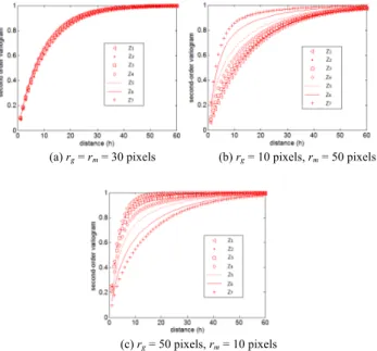
First is for the second-order variogram (Eq. (21)). We set σ2 = 1, ω2
from 0 to 1 with interval 0.125, that is, ω02 = 0, ω12 = 0.125, ..., ω82 = 1. Then we set three examples: (a) rg= rm= 30
10 pixels. When ω02 = 0 and ω82 = 1 the mixture model reduces to single mosaic model and single multi-Gamma model, respectively (not shown). Fig. 3 displays the comparison results.
In (a) it can be seen that the theoretical second-order variograms are close to each other all range of h, it is difficult to distinguish them. In (b) and (c), the theoretical second-order variograms for
Z5 to Z7 can be distinguished when 3 pixels < h < 30 pixels, out of the range they are difficult to be discriminated. Z1 to Z4 are hard to be discriminated in all range of h.
We do the same comparison for the first-order variogram (Eq. (28)). The given parameters’ values are the same as the second-order variogram comparison. Fig. 4 is the comparison results. The first-order variogram of Z7 is very different from the other six ones, so it is not shown in the figure. From the figure we can find that the three results are similar. When 3 < h < 20 (pixel), the first-order variogram for Z1 to Z3 can be distinguished. Z2 and Z6 are mixed with each other and Z3 to Z5 are mixed with each other. After h = 20 pixels, Z2 and Z6 can be discriminated, but Z3 to Z5 are still difficult to discriminated.
Through the comparison above we can know that when rg≠ rmand the weight of Poisson mosaic model is more than 50%,
the mixture model with different values of ω2 can be discriminated by the second-order variogram. When the weight of Poisson mosaic model is less than 50%, the mixture model with different values of ω2 can be discriminated by the first-order variogram.
3.3 Experiment on simulated images
To prove the correctness and accuracy of the first- and second-order variograms, the experiment is performed on simulated images first.
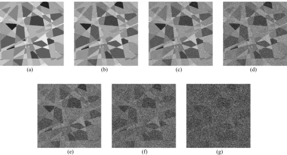
Two basic simulated images are generated from multi-Gamma model and Poisson mosaic model, respectively. Then combine them with different weight parameters ωi2, i = 1, ..., 7,
to generate mixture simulated images.
Fig. 5 shows the two basic simulated images of Poisson mosaic model (Fig. 5 (a)) and multi-Gamma model (Fig. 5 (b)).
Fig. 6 shows simulated images, Fig. 6 (a) - (g) are corresponding to ω72 = 0.875 to ω12 = 0.125, respectively.
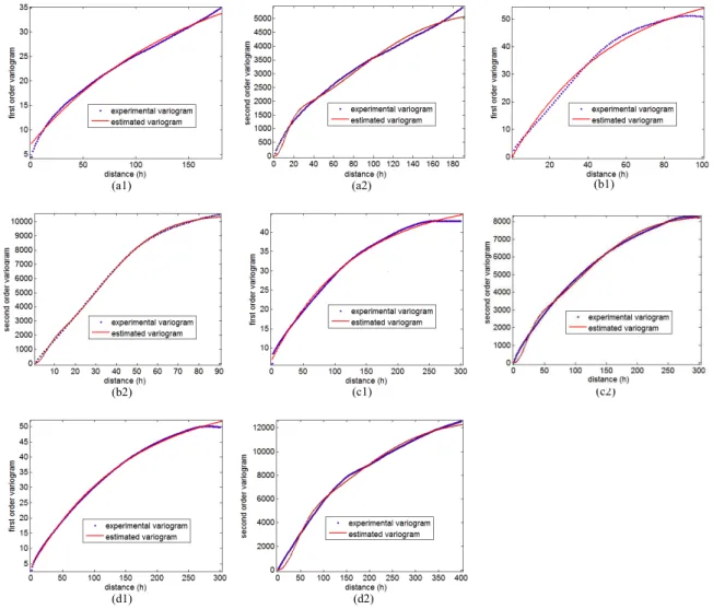
Fig. 7 shows the results of the estimation of the first- and second-order variograms from simulated images. For ω72 = 0.875 to ω12 = 0.125, the theoretical variograms fits well the experimental variograms with accuracy over 90%. Because of the randomness of Gamma model, when h exceeds the R the values of variograms still have some fluctuations. When the weight of Gamma model is over 80%, the fluctuations become obvious.
Table 1 lists the results of estimated parameter ω2
of mixture model Z(x). The values of ω2 are the real weights of the two models, and the values of ωest2 are the estimated weights. From the results, we can find that from Z1(x) to Z3(x) the estimation
results from first-order variogram are more accurate than the second-order variogram’s. But from Z5(x) to Z7(x) the second-order variogram has better estimation results.
Table 1. Parameter (ωest2) of the mixture model Z(x) estimated
from each simulated images.
3.4 Experiment on real sea ice images
The proposed algorithm is tested by using SAR intensity images to identify sea ice structures. Fig. 8 shows the 2-looks Radarsat-1 intensity images, HH polarization and 30 m spatial resolution which is acquired on 12 May 2008 and 26 May 2008 from Hudson Bay, Canada. To validate the rationality of the
random
function Z1 Z2 Z3 Z4 Z5 Z6 Z7
ω2 0.12
5 0.2
5 0.3
6 0.5
0 0.64 0.7
5 0.87
5
first-order-ωest2
0.11 7
0.2 7
0.3 9
0.4 9 0.69
0.7 3
0.80 3
second-order-ωest2
0.16 4
0.2 1
0.2 8
0.5 2 0.67
0.7 8
0.90 4 (b) Multi-Gamma model (a) Poisson mosaic model
Fig.5 Simulated images of two models Fig.3 Experimental second-order variograms computed over images
simulated from the random functions Zi(x), i=1,..., 7. (a) rg = rm = 30 pixels
(c) rg = 50 pixels, rm = 10 pixels
(b) rg = 10 pixels, rm = 50 pixels
Fig.4 Experimental first-order variograms computed over images simulated from the random functions Zi(x), i=1,..., 7.
(c) rg = 50 pixels, rm = 10 pixels
models, we select parts of the two images which are West longitudes from 61° to 65° and North latitudes from 58° to 60°. The egg codes corresponding to the testing images are downloaded from Canadian Ice Service’s website, which provide the information of the sea ice, such as total
concentration, stage of development, form of ice and so on (b)
(a)
(f)
(c) (d)
(e) (g)
Fig.6 Simulated images from different mixture models
Fig.8 RADARSAT-1 SAR image of part of Hudson Bay for (a) May 12 and (b) May 26. Images are superposed with borderlines of ice chart polygons taken from Canadian Ice Service for the same day. Letters in the polygons denote the regions investigated further with the corresponding egg code
given to the right of each image. (a)
(b)
Fig. 9 Polygons cut out from Fig. 8. The white squares of each polygons refer to the samples in Fig. 10 (a) X
.
(b) W
(c) H (d) HH
Fig. 10 Samples of different polygons in Fig. 9
(c) H (d) HH
(Environment Canada 2008). Experiments will be performed for entire polygons, namely X, W, H, HH (Fig. 9), and square-shaped sub-regions of them (Fig. 10).
We choose some polygons which have more representatives for different types of sea ice to do the experiments. Fig. 9 is the
(a1) (a2) (b1)
(b2) (c1) (c2)
(d1) (d2) (e1)
(f1)
(e2) (f2)
(g1) (g2)
Fig.7 Result of the estimations of the first-order and second-order variograms from the simulated images. From (a) to (g) are corresponding to Z1(x) to
polygons of sea ice cut from Fig. 8. Their shapes are irregular and the spatial correlations of them are complicated.
According to the information given in the egg code we can know that even
in one type of sea ice, such as X, there are two or three types of sea ice with different floe size. So in each polygon a square area is selected as a sample used for further experiments. Fig. 10 shows those samples with 100×100 pixels from corresponding polygons in Fig. 9. The samples have regular shape and in their areas the concentrations of sea ice are homogeneous.
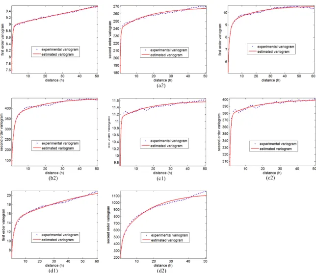
Figs. 11 and 12 display the experimental first- and second-order variograms computed over the polygon images and sample images along with the first- and second-order variograms computed with the estimated parameters of the mixture model.
Tables 2 and 3 list the information (floe size and total concentration) of sea ice derived from egg code and the estimated parameters of the mixture model. The ωest2 of the mixture model is the proportion of the Poisson mosaic structure, which corresponds to the total concentration in the egg code. The R of the mosaic model rm is related to the mean size of the
sea ice, which corresponds to the floe size in the egg code. The R of the multi-Gamma model rg is related to the global texture
structure of the sea. Comparing the estimated results with the information derived from egg code we can find that the parameters in the mixture model can be used to indicate some sea ice parameters.
Table 2. Parameter estimation results of polygons in Fig. 9 types of
sea ice
rg(pixel) rm (pixel)
first-order
second-order
first-order
second-order
H 123.2 134.6 6.8 7.5
HH 113.6 65 1.8 2.6
W 95.3 24 2.8 1.7
X 98.4 111.5 4.2 1.6
floe size(m)
ωest2 total concentr
ation
first-order
second-order
100-500 0.93 0.93 0.9
strips and patches 0.25 0.21 0.2 strips and patches 0.27 0.33 0.3
20-100 0.87 0.91 0.9
Fig. 11 Result of the estimation of the first-order and second-order variograms from polygons (Fig. 9)
(a1) (a2) (b1)
(d1) (d2)
(c1)
Table 3. Parameter estimation results of polygons in Fig. 9
4. DISCUSSION AND CONCLUSION
This paper provides a new method to characterize the spatial structures of sea ice in SAR intensity imagery. The sea ice spatial structures are modeled as a weighted linear combination of two stochastic models: a Poisson line mosaic model and a multi-Gamma model. Then two kinds of geostatistic metrics are defined to describe the image spatial structures. By the experiment, we first compared the theoretical variograms with different values of parameters and found that each of the two different variograms have their own advantages in discriminating different spatial structures. Then the proposed method was applied to the simulated images and RARDARSAT-1 images. Through comparing the parameters estimated from the mixture model with the sea ice information obtaining from egg code, we found that two parameters (concentration and floe size) of sea ice can be retrieved from the mixture model.
Several notes can be remarked from this research. How to estimate other information in the egg code, such as stage of development, is another significant parameter of sea ice. The Voronoi mosaic model is another tessellation model, maybe its way of dividing is more suitable for describing sea ice structures. It will be used to replace Poisson mosaic model in the further study. In the real SAR images, the polygon images are irregular and the sea ice structures are not homogenous, the isotropy assumption is difficult to be satisfied. So the experimental variograms calculated from polygons are not as accurate as the types of
sea ice
rg (pixel) rm (pixel)
first-order
second-order
first-order
second-order
H 75.1 86.5 5.6 6.3
HH 75.6 65.5 3.1 4.3
W 33.2 24.3 3.5 1.7
X 87 95.7 2.6 1.1
floe size(m)
ωest2 total
concentr ation
first-order
second-order
100-500 0.93 0.95 0.9
strips and
patches 0.21 0.23 0.2
strips and
patches 0.33 0.28 0.3
20-100 0.88 0.83 0.9
(c1)
(b2) (c2)
(d1) (d2)
samples’. We should build new models under anisotropy assumption and research them. With the development of the data of remote sensing, the spatial resolution will be higher and higher. The Gamma distribution for modeling the intensity of SAR image is not applicable. Instead of Gamma distribution, some elaborate statistic distributions, for example: K distribution (Keith et al. 2006), are needed for the purpose.
REFERENCES
Bernardoff P. (2006). Which multivariate gamma distributions are infinitely divisible? Bernoulli, 12(1), 169–189.
Chiles J., & Delfiner P. (1999). Geostatistics Modeling Spatial Uncertainty. New York, America: Wiley.
Clausi D. A., & Deng H. (2003). Operational segmentation and classification of SAR sea ice imagery. IEEE Workshop on Advances in Techniques for Analysis of Remotely Sensed Data. 268-275.
Emilio C., Jonathan L., & Yang X. (2010). Advances in Earth Observation Global Change. (1st edition). German: Springer.
Environment Canada (2008). Canadian Ice Service, Latest Ice Condition. http:// www.ec.gc.ca /glaces-ice/default.asp?lang=En&n=D32C361E-1
Feng Y. (2008). Application of Spatial Statistics Theory and its Application in Forestry. Beijing, China: China Forestry Press.
Garrigues S., Allard D., & Baret F. (2007). Using first- and second-order variograms for characterizing landscape spatial structures from remote sensing imagery. IEEE Transactions on Geoscience and Remote Sensing, 45(6), 1823-1834.
Garrigues S., Allard D., Baret F., & Weiss M. (2006). Quantifying spatial heterogeneity at the landscape scale using variogram models. Remote Sensing of Environment, 103(1), 81–96.
Johannessen O. M., Alexandrov V. Y., Frolov I. Y., Sandven S., Pettersson L. H., Bobylev L. P., Kloster K., Smirnov V. G., Mironov Y. U., & Babich N. G. (2007). Remote sensing of sea ice in the northern sea route studies and applications. Springer and Praxis Publishing.
Keith D. W., Robert J. A. T., & Simon W. (2006). Sea Clutter: Scattering, the K Distribution and Radar Performance. London, United Kingdom: The Institution of Engineering and Technology.
Kerman B. R. (1999). Information states in radar imagery of sea ice. IEEE Transactions on Geoscience and Remote Sensing, 37(3), 1435–1446.
Kotz S., Balakrishnan N., & Johnson N. L. (2000). Continuous multivariate distributions: models and applications. (2nd edition). New York, America: Wiley.
Lantuéjoul C. (2002). Geostatistical Simulation Models and Algorithms. German: Springer.
Nystuen J. A., & Garcia Jr. F. W. (1992). Sea ice classification using SAR backscatter statistics. IEEE Transactions on Geoscience and Remote Sensing, 30(3), 502-509
Ochilov S., & Clausi D. A. (2012). Operational SAR sea-ice image classification. IEEE Transactions on Geoscience and Remote Sensing, 50(11), 4397-4408.
Schabenberger O., & Gotway C. A. (2005). Statistical Methods for Spatial Data Analysis. England: Chapman and Hall/CRC.
Sheldon M. R.(2004). Introduction to Probability and Statistics for Engineers and Scientists. (3rd edition). America: Academic Press.
Soh L., & Tsatsoulis C. (1999). Texture analysis of SAR sea ice imagery using gray level co-occurrence matrices. IEEE Transactions on Geoscience and Remote Sensing, 37(2), 780-795.
Wackernagel H. (1998). Multivariate Geostatistics: an Introduction with Applications. (2nd edition). German: Springer.
Zhang Y. (1983). The joint distribution function of the sum and difference of two Gamma distributed random variables independent of each other. Journal of Hefei Polytechnic University, (3), 53-59.
Zhang Y., Hu R., Sun J., & Mao S. (2010). Change detection for SAR images based on bivariate Gamma models. Systems Engineering and Electronics, 32(5), 927-930