EVALUATION OF TWO SEMI-ANALYTICAL TECHNIQUES IN AIR
QUALITY APPLICATIONS
JONAS C. CARVALHO
1& DAVIDSON M. MOREIRA
21
Universidade Federal de Pelotas, Faculdade de Meteorologia, PPGMET, Pelotas-RS, Brasil
E-mail: [email protected]. Phone: 0055 53 32776690, FAX 0055 53 32776722.
2Universidade Federal do Pampa, Centro de Ciência Exatas e Tecnológicas, Bagé-RS, Brasil
Received August 2004 - Accepted July 2005
ABSTRACT
In this article an evaluation of two semi-analytical techniques is carried out, considering the quality and accuracy of these techniques in reproducing the ground-level concentration values of passive pollutant UHOHDVHGIURPORZDQGKLJKVRXUFHV7KH¿UVWWHFKQLTXHLVDQ(XOHULDQPRGHOEDVHGRQWKHVROXWLRQ of the advection-diffusion equation by the Laplace transform technique. The second is a Lagrangian model based on solution of the Langevin equation through the Picard Iterative Method. Turbulence parameters are calculated according to a parameterization capable of generating continuous values in all stability conditions and in all heights of the planetary boundary layer. Numerical simulations and comparisons show a good agreement between predicted and observed concentrations values. Comparisons between the two proposed techniques reveal that Lagrangian model generated more accurate results, but Eulerian model demands a lesser computational time.
Keywords: semi-analytical technique, Eulerian model, Lagrangian model, Laplace transform, Picard Iterative Method, model evaluation.
RESUMO:AVALIAÇÃO DE DUAS TÉCNICAS SEMI-ANALÍTICAS EM APLICAÇÕES NA QUALIDADE DO AR.
Neste artigo é realizada uma avaliação de duas técnicas semi-analíticas, considerando a qualidade e a exatidão destas técnicas em reproduzir valores de concentração ao nível da superfície de poluentes passivos emitidos a partir de fontes baixas e altas. A primeira técnica é um modelo Euleriano baseado na solução da equação advecção-difusão através da técnica de transformada de Laplace. A segunda é um modelo Lagrangiano baseado na solução da equação de Langevin através do Método Iterativo de Picard. Parâmetros da turbulência são calculados de acordo com uma parametrização capaz de gerar valores contínuos em todas as condições de estabilidade e em todas as alturas na camada limite planetária. Simulações numéricas e comparações mostram uma boa concordância entre valores de concentração previstos e observados. Comparações entre as duas técnicas revelam que o modelo Lagrangiano gera resultados mais precisos, mas o modelo Euleriano exige um menor tempo computacional.
Palavras-chave:técnica semi-analítica, modelo Euleriano, modelo Lagrangiano, transformada de Laplace, Método Iterativo de Picard, avaliação de modelos.
1. INTRODUCTION
Currently, the search for analytical solutions for the dispersion problems is one of the main research subjects in the pollutant dispersion modelling. These solutions become important due to the intention to obtain dispersion models that generate reliable results in a small computational time, which are of great iterest for regulatory air quality applicarions. $QDO\WLFDOVROXWLRQVEHLQJWKHLQÀXHQFLQJSDUDPHWHUVH[SOLFLWO\
expressed in a mathematical closed form, allow in general a deep sensitivity analysis over model parameters. Moreover, computer codes based on analytical expressions in general do not have to consider prohibitive computational resources.
solutions of the diffusion-advection equation they are assumed constant along the whole Planetary Boundary Layer (PBL) or following a power law (van Ulden, 1978; Pasquill and Smith, 1983; Seinfeld, 1986; Tirabassi et al., 1986; Sharan et al., 1996). In Lagrangian particle models, the solution of the Langevin equation is normally obtained according to the rulesis normally obtained according to the rules of the Ito calculus (Rodean, 1996). Some special solutions of the Langevin equation are presented by Gardiner (1985) and Rodean (1996). This last author, for instance, describes the solution for stationary homogeneous turbulence as suggested by Lin and Reid (1963) and Legg and Raupach (1982).
In this paper two semi-analytical techniques are used to simulate the pollutant dispersion during two tracer dispersion H[SHULPHQWV7KH¿UVWWHFKQLTXHLVDQ(XOHULDQPRGHOEDVHG on a discretization of the PBL in N layers; in each sub-layers the advection-diffusion equation is solved by the Laplace transform technique, considering an average value for eddy diffusivity and the wind speed. (Vilhena et al.,1998; Moreira et al.,1999). The second technique is based on solution of the Langevin equation through the Method of Successive Approximations or Picard’s Iteration Method (Carvalho et al., 2004, 2005). Lagrangian particle models are obtained considering the Gram-Charlier Probability Density Function (PDF) of turbulent velocity, through which Gaussian and non-Gaussian turbulence conditions can be considered (Anfossi et al., 1997; Ferrero and Anfossi, 1998). The main objective of this paper is to present and discuss the results of a model evaluation between two semi-analytical techniques, focusing the quality and accuracy of these techniques in UHSURGXFLQJWKHJURXQGOHYHOFRQFHQWUDWLRQ¿HOGRIDSDVVLYH pollutant emitted from low and high sources. Furthermore, this work presents the mathematical and computational features of the Eulerian and Lagrangian models to provide a better understanding about these two techniques.
The turbulent parameters used as input in Eulerian model (diffusion coefficients) and Lagrangian model YHORFLW\ÀXFWXDWLRQVPRPHQWVDQG/DJUDQJLDQGHFRUUHODWLRQ time scales) are parameterized according to a scheme able to generate continuous values in all stability and in all heights in the PBL (Degrazia et al., 2000). Ground-level concentrations measured during Prairie Grass (Barad, 1958) and Copenhagen (Gryning and Lyck, 1984) experiments are used to compare observed and calculated concentrations. The results are evaluated through a statistical analysis ordinarily used to evaluate pollutant dispersion models (Hanna, 1989). The paper is outlined as follows: in section two we present the description of the models, in section three we report the turbulence parameterization, in section four we display the modelling results attained by the two semi-analytical methods DQGLQVHFWLRQ¿YHZHSUHVHQWWKHFRQFOXVLRQV
2. DESCRIPTION OF THE MODELS
2.1. Eulerian Model
Following Vilhena et al. (1998) and Moreira et al. (1999), the steady state advection-diffusion equation is written as (Arya, 1995):
U C
x x K
C x i i i i i u u u u u u ¥ § ¦¦ ¦¦ ´ ¶ µµµ
µ, (1)
where i = 1, 2, 3, C denotes the average concentration, xi is
the position, Ui is the mean wind velocity and Ki is the eddy
diffusivity. The cross-wind integration of the Equation (1), in which the longitudinal axis coincides with the direction of the average wind and the longitudinal diffusion is neglected, leads to:
U C
x x K
C x y y 1 1 3 3 3 u u u u u u ¥ § ¦¦ ¦¦ ´ ¶ µµµ
µ, (2)
VXEMHFWWRWKHERXQGDU\FRQGLWLRQVRI]HURÀX[DWWKHJURXQGDQG PBL top, and a source with emission rate Q at height Hs:
K C x y 3 3 0 u
u in x3 = 0,h (3)
U C1 y(0, x3)= Q xE( 3Hs) in x1 = 0, (4)
where now Cy represents the average cross-wind integrated
concentration,Q is the source term and D is the delta Dirac. Bearing in mind the dependence of the K3 and U1 on the
variable z, the height h of PBL is discretized in N sub-intervals in such a manner that inside each interval Kz(z) and U(z) assume
the average value: K
x x K x dx
n n n x x n n
°
1 3 31 3 3 3
31 3
( ) (5)
U
x x U x dx
n n n x x n n
°
1 3 31 1 3 3
31 3
( ) . (6)
Therefore, the solution of problem (2) is reduced to the solution of N problems of the type:
U C x K C x n y n n y n u u u u 1 2 3 2
xn x xn
3 1
3 3
, (7)
for n = 1:N, where Cny denotes the concentration at the nth
subinterval. To determine the 2N integration constants the additional (2N-2) conditions namely continuity of concentration DQGÀX[DWWKHLQWHUIDFHDUHFRQVLGHUHG
Cyn C y n
1 n = 1,2,… (N – 1) (8)
K C x K C x n y n n y n u u u u 3 1 1 3
u u
2
3
2 3 3 0 3
x C s x U s
K C s x
U
K C x
y n n n y n n n y n
( , ) ( , ) ( , ), (10)
where C s xy L C x x x s n
p y n
( , 3)
\
( ,1 3); 1m^
and Lp is the operatorof the Transform Laplace. The well-known solution of the Equation (10) is (Boyce and DiPrima, 1999):
C s x A e B e Q
R e e
y
n n R x n R x a
R x H R x H
n n n
s n s
( , 3) ( ) ( )
3 3 3 3
2
(11) where
R U s
K R U K s
n n
n a
n n
and .
Finally, applying the interface and boundary conditions we come out with a linear system for the integration constants. Henceforth the concentration is obtained inverting numerically the transformed concentration Cy by Gaussian quadrature
scheme (Heydarian and Mullineaux, 1989):
C x x A P
x A e B e
y n
k k n
P U x K x n
P U x
k n
n
k n
( ,1 3)
1 1 3 1 ¥ § ¦¦¦ ¦¦¦ ´ ¶ µµµ
µµµµ KK x
k
Nk n
¥ § ¦¦¦ ¦¦¦ ´ ¶ µµµ µµµµ ¨ ª © © © © · ¹ ¸ ¸ ¸ ¸
¤
3 1 (12)C x x A P
x A e B e
y n
k k n
P U x K x n
P U x
k n
n
k n
( ,1 3)
1 1 3 1 ¥ § ¦¦¦ ¦¦¦ ´ ¶ µµµ
µµµµ KK x
k N k n n n k Q P K U
x e ¥ § ¦¦¦ ¦¦¦ ´ ¶ µµµ µµµµ ¨ ª © © © © · ¹ ¸ ¸ ¸ ¸
¤
3 1 1 1 2( xx H P U
x K x H P U x K
s k
n
n s k
n n e 3 1 3 1 ¥ § ¦¦¦ ¦¦¦ ´ ¶ µµµ
µµµµ ¥ § ¦¦¦ ¦¦¦ ´ ) ( ) ¶¶ µµµ µµµµ ¥ § ¦¦ ¦¦ ¦¦ ¦¦ ´ ¶ µµµ µµµ µµ · ¹ ¸ ¸ ¸ ¸ ¸ ¸ ¸ . (13)
The solution (12) is valid for layers that do not contain the contaminant source and x1 > 0, once the quadrature scheme
of Laplace inversion does not work for and x1 = 0. On the other
hand, the solution (13) can be used to evaluate the concentration ¿HOGLQWKHOD\HUWKDWFRQWDLQVWKHFRQWLQXRXVVRXUFH$k and Pk
are the weights and roots of the Gaussian quadrature scheme and are tabulated in the book by Stroud and Secrest (1966).
2.2. Lagrangian Model
An alternative method to solve the Langevin equation based on Picard’s Iterative Method was suggested by Carvalho et al. (2004). The three dimensional Langevin equation for inhomogeneous turbulence is:
du
dt a x u b x u t i
i i i i i i i
( , ) ( , ) ( )Y , (14a) where ui is the turbulent velocity component of each particle,
ai(xi, ui)dt is the deterministic term, bi(xi, ui)Xi(t) is the stochastic
term and Xi is a normally distributed (average 0 and variance dt)
random increment. The displacement of each particle is given by:
dxi Uiu dti
. (14b)Therefore, the Langevin model consists of a pair of stochastic differential equations that describe the trajectories of QHXWUDOO\EXR\DQW³PDUNHGSDUWLFOHV´LQWKHÀXLG5RGHDQHWDO 1992). This formulation includes the well-mixed criterion, which declaretes that if a species of passive “marked particles” is initially mixed uniformly in position and velocity space in DWXUEXOHQWÀRZKRPRJHQHQRXVRULQKRPRJHQHRXVLWZLOO stay that way (Thomson, 1987). The particles are not allowed to interact among themselves and no deposition or buoyance effects participe of the dynamic of this model.
,Q/DQJHYLQHTXDWLRQWKHGHWHUPLQLVWLFFRHI¿FLHQWa depends on the Eulerian PDF of the turbulent velocity and is determined from the Fokker-Planck equation under steady conditions for the statistical momentum (Thomson, 1987; Rodean, 1996). A Gram-Charlier PDF, which is given by the series of Hermite polynomials, can be adopted (Anfossi et al., 1997; Ferrero and Anfossi, 1998). The Gram-Charlier PDF truncated to the fourth order is given by the following expression (Kendall and Stuart, 1977):
P ri e C H r C H r r
i i
i
( )
<
( ) ( )>
2 2
3 3 4 4
2Q 1 (15)
where ri = ui/Si,Si is the turbulent velocity standard deviation,
H3 and H4 are the Hermite polynomials and C3 and C4 their
FRHI¿FLHQWVREWDLQHGDFFRUGLQJWR C
m P r H r dr m
m
d d
°
1
! . (16)
In the case of Gaussian turbulence, Equation (15) becomes a normal distribution, considering C3 and C4 equal
to zero. The third order Gram-Charlier PDF is obtained with C4 = 0.
Applying the Equation (15) in steady Fokker-Planck HTXDWLRQWKHGHWHUPLQLVWLFFRHI¿FLHQWLVJLYHQE\ a f h x g h i i i i L i i j i i i u u T U T T
, (17)
where j can assume 1, 2, 3 and j x i, TLi is the Lagrangian
decorrelation time scale and fi, gi and hi are expressions written
as:
fi 3C3ri 15C4 1 6C r3i 10C ri C ri C ri 2 4 3 3 4 4 5 ( ) (18a) gi 1 C4ri 1C 2C ri 5C ri C ri C ri
2 4 3 3 4 4 3 5 4 6 ( ) (18b) hi 1 3C43C r3i6C r4i2C ri C ri
3 3
4 4
. (18c)
du dt f h x g h t i i i i L i i j i i i L i i i u u ¥ § ¦¦ ¦¦¦ ´ ¶ µµµ µµ T U T T T U Y
2 2 1 2
( ), (19)
assuming that bi i L
i
2T U2
1 2(Hinze, 1975; Tennekes, 1982), where Ti2 is the turbulent velocity variance.
Rewriting the Equation (19) as du
dt u t
i
i i i i i L i i ¥ § ¦¦ ¦¦¦ ´ ¶ µµµ µµ
B C H T
U Y
2 2 1 2
( ), (20)
where B U i i L C h i
15 41, C T
U i i i
i i L
f r C
h
i
[ (15 41)]1 and
Hi Ti T i j i i x g h u u ,
it is possible to determine exp( Bi ) t
t ds
0
°
as the integrating factor for the Equation (20).Multiplying the integrating factor by all terms in Equation (20), we obtain an integral equation
ui ids ds
t t i t t ¥ § ¦¦ ¦¦¦ ´ ¶ µµµ µµµ ¥ § ¦¦ ¦¦¦ ´ ¶ µµµ µ
°
°
exp exp ’ B B0 0 µµµ
« ¬ ®®® ®®®
°
tt 0
¨ ª© · ¹¸ º » ®®® ¼ Ci Hi 2T Ui Li Yi t dt2 1 2
( )’ ’
®®®®, (21a)
from which the iterative approximation presents the following form:
ui ds u ds
n i n t t i n i n t t ¥ § ¦¦ ¦¦¦ ´ ¶ µµµ µµµ ¥ § ¦¦ ¦¦¦
°
°
1 0 0 exp exp ’B B ´´
¶ µµµ µµµ « ¬ ®®® ®®
°
t t0 ®® ¨ª©Ci H T U Y ·¹¸ n
i n
i L i n
i t dt
2 2 1 2
( )’ ’ º » ®®® ¼
®®®. (21b)
The Picard´s Iteration Method (Boyce and DiPrima, 1999; page 69) is applied to the Equation (21), assuming that the initial value for the turbulent velocity is a random value supplied by a Gaussian distribution. The Picard Iterative Method or Method of Successive Approximations is a numerical process that can approximate the solution of an initial problem value. The method generates a sequence of functions through a recurrent formula, which converges to the solution of the initial problem value. The sequence of functions obtained through the iterative process converges to a unique solution provided the Lipschitz condition LVVDWLV¿HGWKDWLVLIWKHUHLVDFRQVWDQWc such that
f t x t, 1( )
f t x t, 2( )bc x t1( )x t2( ) . (22) In principle, the Picard’s Iteration Method can be applied to any differential equation, and by this reason is proof of existence and uniqueness of a solution (Innocentini, 1999).3. TURBULENCE PARAMETERIZATION
The present application considers the turbulence parameterization scheme suggested by Degrazia et al. (2000). Accounting for the current knowledge of the PBL structure and characteristics, the authors derived parameterizations for eddy difusivity (Ki), turbulent velocity variance (Ti
2
) and Lagrangian decorrelation time scale (TLi):
K c z
z h L h h L w f i i c m ¥ §
¦¦¦ ´¶µµµ ¥§¦¦¦¦ ´ ¶ µµµ
µ
0 14
1 3 1 2
.
[(
ZF
)) ]i [( ) ] c n s m i n s u f 4 3 1 3 4 3
« ¬ ®® ®® ®®® ®® ®® ®®® º » ®® ®® ®®GF ®®
¼ ®® ®® ®®® (23) ˆ
. c ¨ z
h w
f
. c ˘ i i c * m i c i 2 2 3 2 2 3
1 06 2 32
¥ § ¦¦¦ ´¶µµµ
¨ ª© · ¹¸ n s m i n s u f
¨ ª© · ¹¸
2 3 2
2 3 (24)
and U ZF L i m i c c i z c L h h L
f w z
h ¥ § ¦¦ ¦¦ ´ ¶ µµµ µ ¥ § ¦¦¦ 0 14 1 2 2 3 . [( ) ] ´´ ¶ µµµ
« ¬ ®® ®® ®®® ®® ®® ®®® º1 3 2 3 1 3
0 059. [(fm i)n s] Gn s u
F »» ®® ®® ®®® ¼ ®® ®® ®®® (25) where the superscripts c, n and s indicate convective, neutral and stable, respectively, h is the PBL height,w* is the convective velocity scale, u* is the local friction velocity,
ZF F c
h w
/
3 and G FL F n s
z u
( ) / 3 are the nondimensional molecular dissipation rate functions associated to buoyancy and mechanical productions, respectively, E is the dissipation rate of turbulent kinetic energy, (fm i)
c
is the reduced frequency of
the convective spectral peak, (f ) m i
n s
is the reduced frequency
of the neutral or stable spectral peak, L is the Monin-Obukohv length, –L
_
/h is an average stability parameter for the convective PBL, in which a typical value of 0.01 is used (this term is introduced in order to give a continuous transition from neutral to convective conditions), K is the Von Karman constant and
ci i u
B B (2QL) 2 3 with B
u0 5. p0 05. and AI= 1,4/3,4/3
for u, v and w components, respectively.
4. MODELLING RESULTS
4.1. Comparison with Prairie Grass Data Set -
Unstable Case
The Prairie Grass experiment was realized in O’Neill, Nebraska, 1956. The pollutant (SO2) was emitted without
buoyancy at a height of 0.5 m and it was measured by samplers DWDKHLJKWRIPLQ¿YHGRZQZLQGGLVWDQFHV P7KH3UDLULH*UDVVVLWHZDVÀDWZLWKDURXJKQHVV length of 0.6 cm. The results for twenty convective (–h/L > 10) experiments are presented. All available data (see Table 1) ZHUHXVHGWRFUHDWHDLQSXW¿OHIRUWKHVLPXODWLRQV:LQGVSHHG SUR¿OHKDVEHHQSDUDPHWHUL]HGIROORZLQJWKHVLPLODULW\WKHRU\RI Monin-Obukhov and OML model (Berkowicz et al., 1986).
)RUWKHVLPXODWLRQVWKHWXUEXOHQWÀRZZDVDVVXPHG inhomogeneous only in the vertical and the transport was realized by the longitudinal component of the mean wind velocity. The horizontal domain was determined according to sampler distances and the vertical one was set equal to the observed PBL height. In Eulerian model, the order of the Gaussian quadrature scheme was Nk = 8 because this value
provides the desired accuracy with the smallest computational
time. The number of sub-layers N is set according to desired accurate (Moreira et al., 2005); obviously, the greater is N the more accurate is the calculated concentration pattern, but as a consequence the greater is the relative computational time. In Lagrangian models, the time step was maintained constant and it was obtained according to the value of the Lagrangian decorrelation time scale ($t = TL/ 10), where TL must be the
smaller value between its components. The boundary condition SHUPLWVUHÀHFWLRQRISDUWLFOHYHORFLW\DWWKHWRSDQGDWWKHERWWRP of the simulation domain. In Gaussian turbulence case the SHUIHFWUHÀH[LRQLVFRQVLGHUHGDQGLQQRQ*DXVVLDQWXUEXOHQFH case the scheme suggested by Thomson and Montgomery (1994) is used. Fifty particles were released in each time step during WLPHVWHSV7KHFRQFHQWUDWLRQ¿HOGZDVGHWHUPLQHG by counting the particles in a cell or imaginary volume. The integration method used to solve the integrals appearing in Equation (21) was the Romberg technique.
The model performances are shown in Tables 4 and 5 and Figures 1a and 2a. Table 4 shows the result of the statistical analysis made with the observed and predicted values of ground-level cross-wind-integrated concentration (Cy). Table 5 Table 1 – Meteorological parameters and concentrations measured during the Prairie Grass unstable experiment. Q is the emission rate and Cy is
the ground-level cross-wind-integrated concentration.
run -L
(m)
h (m)
w*
(ms-1)
U 10 m (ms-1)
Q (gs-1)
Cy 50 m
(gm-2)
Cy 100 m
(gm-2)
Cy 200 m
(gm-2)
Cy 400 m
(gm-2)
Cy 800 m
(gm-2)
1 9 260 0.84 3.2 82 7.00 2.30 0.51 0.16 0.062
5 28 780 1.64 7.0 78 3.30 1.80 0.81 0.29 0.092
7 10 1340 2.27 5.1 90 4.00 2.20 1.00 0.40 0.18
8 18 1380 1.87 5.4 91 5.10 2.60 1.10 0.39 0.14
9 31 550 1.70 8.4 92 3.70 2.20 1.00 0.41 0.13
10 11 950 2.01 5.4 92 4.50 1.80 0.71 0.20 0.032
15 8 80 0.70 3.8 96 7.10 3.40 1.35 0.37 0.11
16 5 1060 2.03 3.6 93 5.00 1.80 0.48 0.10 0.017
19 28 650 1.58 7.2 102 4.50 2.20 0.86 0.27 0.058
20 62 710 1.92 11.3 102 3.40 1.80 0.85 0.34 0.13
25 6 650 1.35 3.2 104 7.90 2.70 0.75 0.30 0.063
26 32 900 1.86 7.8 98 3.90 2.20 1.04 0.39 0.127
27 30 1280 2.08 7.6 99 4.30 2.30 1.16 0.46 0.176
30 39 1560 2.23 8.5 98 4.20 2.30 1.11 0.40 0.10
43 16 600 1.66 6.1 99 5.00 2.40 1.09 0.37 0.12
44 25 1450 2.20 7.2 101 4.50 2.30 1.09 0.43 0.14
49 28 550 1.73 8.0 102 4.30 2.40 1.16 0.45 0.15
50 26 750 1.91 8.0 103 4.20 2.30 0.91 0.39 0.11
51 40 1880 2.30 8.0 102 4.70 2.40 1.00 0.38 0.084
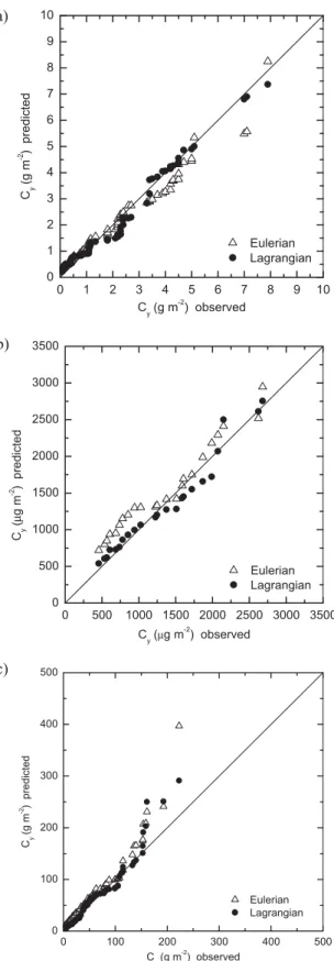
presents the computational time comparison between Eulerian and Lagrangian models. Figure 1a shows the scatter diagram between observed and predicted Cy, where lines have been added
to indicate factor of two and factor of three under and over prediction. Figure 2a shows a quantile-quantile plot where the distribution of predicted and observed values are compared. The data are ordered by rank, so for instance the highest observed concentration is paired with the highest predicted concentration (Olesen, 1995). In this sense, this plot permits to compare the frequency distributions of predicted and observed data. The statistical indices in Table 4 are the following (Hanna, 1989):
NMSE(CoCp) /C Co p 2
(Normalized Mean Square Error) FB(CoCp) /( . (0 5CoCp))
(Fractional Bias) FS2 ToTp
ToTp (Fractional Standard Deviation)R(CoCo)(CpCp) /T To p &RUUHODWLRQ&RHI¿FLHQW
FA2 = fraction of the data for which 0 5. bCp Cob2 (Factor of Two)
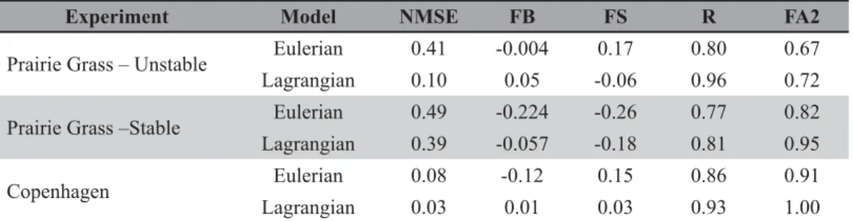
where C is the analyzed quantity (concentration) and the subscripts “o” and “p” represent the observed and the predicted values, respectively. The overbars in the statistical indices indicate averages. The statistical index FB indicates if the predicted quantity underestimates or overestimates the observed one. The statistical index NMSE represents the quadratic error of the predicted quantity in relation to the observed one. The statistical index FS indicates the measure of the comparison between predicted and observed plume spreading. The statistical index FA2 provides the fraction of data for which 0 5. bC Co pb2. As nearest zero are the NMSE, FB and FS and as nearest one are the R and FA2, better are the results.
According Table 4 and 5 and Figures 1a and 2a, the results show a satisfactory agreement between measurements and simulations. NMSE, FB and FS values are relatively near to zero and R and FA2 are relatively near to 1. The Lagrangian model presents a better performance than Eulerian model when observed and predicted concentration values are compared. However, the computational time required by the Eulerian model to simulate all runs is approximately sixty times lesser.
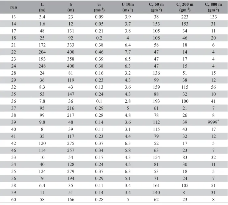
4.2. Comparison with Prairie Grass Data Set - Stable
Case
The tracer (SO2) was released without buoyancy at
a height of 0.5 m and collected at a height of 1.5 m at three
downwind distances (50, 200 and 800 m). The Prairie Grass site ZDVTXLWHÀDWDQGPXFKVPRRWKZLWKDURXJKQHVVOHQJWKRI FP:HSUHVHQWKHUHWKHUHVXOWVIRUWZHQW\VHYHQVWDEOHUXQV IRUZKLFKWKHFRQGLWLRQK/!LVVDWLV¿HGVHH7DEOH7KH micrometeorological parameters recorded during the dispersion experiments are summarized in Table 3, based on the paper of YDQ8OGHQ7KHZLQGVSHHGSUR¿OHLVSDUDPHWHUL]HG following the similarity theory of Monin-Obukhov and OML model (Berkowicz et al., 1986). The numerical and computational characteristics to simulate the Prairie Grass stable experiment were the same used to simulate the unstable one. The results provided by the simulations can be seen in Tables 4 and 5 and Figures 1b and 2b. Like it happened in the unstable Prairie Grass simulation, the Lagrangian model presents accurate results when compared with the ones generated by the Eulerian model. However, the computational effort of the Eulerian model demands a lesser computational time.
4.3. Comparison with Copenhagen Data Set
The Copenhagen experiment was carried out in the northern part of Copenhagen. The pollutant (SF6) was
released without buoyancy from a tower at a height of 115 m and collected at the ground-level positions in up to three crosswind arcs of tracer sampling units. The sampling units were positioned 2-6 km from the point of release. The site was mainly residential with a roughness length of 0.6 m. The results for nine runs performed under neutral to convective conditions DUHSUHVHQWHGVHH7DEOH:LQGVSHHGVDWDQGPHWHUV ZHUHXVHGWRFDOFXODWHWKHFRHI¿FLHQWIRUWKHH[SRQHQWLDOZLQG YHUWLFDOSUR¿OH7KHQXPHULFDODQGFRPSXWDWLRQDOFKDUDFWHULVWLFV to simulate the Copenhagen experiment were the same used to simulate the Prairie Grass experiment. The results provided by the simulations show a very good agreement with measured data. Again, the simulations revealed that, in general, Lagrangian model generates more accurate results, but the simulation time UHTXLUHGE\WKH(XOHULDQPRGHOLVVLJQL¿FDQWO\VPDOOHUDVFDQ be seen in Tables 4 and 5 and Figures 1c and 2c.
4.4. Mathematical and Computational Analysis
To a better understanding of the numerical comparison between the Eulerian and Lagrangian semi-analytical methods in this work, our attention is now focused to the mathematical and computational feature of these approaches. Concerning the Eulerian model, it is well known that the results attained by the Gaussian quadrature scheme of order Nk, are exact when the
transformed function is a polynomial of degree (2 Nk – 1). On
Table 2 – Meteorological parameters and concentrations measured during the Prairie Grass stable experiment.
run L
(m)
h (m)
u*
(ms-1)
U 10m (ms-1)
Cy 50 m
(gm-2)
Cy200 m200 m
(gm-2)
Cy800 m800 m
(gm-2)
13
3.4
23
0.09
3.9
38
223
133
14
1.6
12
0.05
3.7
153
153
31
17
48
131
0.21
3.8
105
34
11
18
25
92
0.2
4
108
46
20
21
172
333
0.38
6.4
58
18
6
22
204
400
0.46
7.7
47
14
4
23
193
358
0.39
6.5
47
17
4
24
248
400
0.38
6.3
47
15
4
28
24
81
0.16
3.2
136
51
15
29
36
119
0.23
4.3
99
38
12
32
8.3
43
0.13
3.6
159
115
56
35
53
147
0.24
4.3
88
32
10
36
7.8
36
0.1
2.8
193
100
41
37
95
216
0.29
5
61
21
7
38
99
217
0.28
4.8
78
26
8
39
9.8
48
0.14
3.6
112
39
9999
*40
8
39
0.11
3.1
115
43
17
41
35
117
0.23
4.4
79
32
12
42
120
275
0.37
6.3
52
17
5
46
114
257
0.34
5.8
63
23
7
53
10
54
0.17
4.3
154
83
32
54
40
128
0.24
4.5
81
30
11
55
124
279
0.37
6.3
53
18
5
56
76
194
0.29
5.1
71
24
7
58
6.4
35
0.11
3.4
161
105
51
59
11
51
0.14
3.4
140
81
31
60
58
166
0.28
5
62
23
8
*missing data
a polynomial, with the property that a better approximation is achieved with the increasing of the degree of the polynomial. This means that increasing Nk in the Gaussian quadrature
schemes appearing in the concentration solution given by Equations (12) and (13), it is expected that the numerical results should converges for the exact result. Concerning the issue of stepwise approximation, it is important to bear in mind that the stepwise approximation of a continuous function converges to the continuous function, when the stepwise of the approximation goes to zero. Therefore, for the Eulerian model it
is only necessary to choose the number of the sub-layers in an appropriate manner, by taking the smoothness of the continuous functions K3 and U1 into account.
Tabela 3 – Meteorological parameters and concentrations measured during the Copenhagen experiment.
run -L
(m)
h (m)
u*
(ms-1)
U 10 m (ms-1)
U 115 m (ms-1)
Q (gs-1)
distance (m)
Cy
(µgm-2)
1
37
1980
0.36
2.1
3.4
3.2
1900
2074
1
37
1980
0.36
2.1
3.4
3.2
3700
739
2
292
1920
0.73
4.9
10.6
3.2
2100
1722
2
292
1920
0.73
4.9
10.6
3.2
4200
944
3
71
1120
0.38
2.3
5.0
3.2
1900
2624
3
71
1120
0.38
2.3
5.0
3.2
3700
1990
3
71
1120
0.38
2.3
5.0
3.2
5400
1376
4
133
390
0.38
2.5
4.6
2.3
4000
2682
5
444
820
0.45
3.1
6.7
3.2
2100
2150
5
444
820
0.45
3.1
6.7
3.2
4200
1869
5
444
820
0.45
3.1
6.7
3.2
6100
1590
6
432
1300
1.05
7.2
13.2
3.1
2000
1228
6
432
1300
1.05
7.2
13.2
3.1
4200
688
6
432
1300
1.05
7.2
13.2
3.1
5900
567
7
104
1850
0.64
4.1
7.6
2.4
2000
1608
7
104
1850
0.64
4.1
7.6
2.4
4100
780
7
104
1850
0.64
4.1
7.6
2.4
5300
535
8
56
810
0.69
4.2
9.4
3.0
1900
1248
8
56
810
0.69
4.2
9.4
3.0
3600
606
8
56
810
0.69
4.2
9.4
3.0
5300
456
9
289
2090
0.75
5.1
10.5
3.3
2100
1511
9
289
2090
0.75
5.1
10.5
3.3
4200
1026
9
289
2090
0.75
5.1
10.5
3.3
6000
855
Table 4 – Statistical indices of the model performance for the Prairie Grass and Copenhagen experiments.
Experiment Model NMSE FB FS R FA2
Prairie Grass – Unstable Eulerian 0.41 -0.004 0.17 0.80 0.67
Lagrangian 0.10 0.05 -0.06 0.96 0.72
Prairie Grass –Stable Eulerian 0.49 -0.224 -0.26 0.77 0.82
Lagrangian 0.39 -0.057 -0.18 0.81 0.95
Copenhagen Eulerian 0.08 -0.12 0.15 0.86 0.91
Lagrangian 0.03 0.01 0.03 0.93 1.00
Table 5 – Computational time comparison between Eulerian and Lagrangian models.
model computational time (s)
Prairie Grass - Unstable Prairie Grass - Stable Copenhagen
Eulerian 30 10 10
Figure 1 – Scatter diagram between observed and predicted Cy for the
(a) Prairie Grass unstable (b) Prairie Grass stable and (c) Copenhagen
experiments. Dashed lines indicate factor of 2, dotted lines indicated factor of 3 and solid line indicates unbiased prediction.
Figure 2 – Model perfomance in terms of quantile-quantile. (a) Prairie
Grass unstable, (b) Prairie Grass stable and (c) Copenhagen
experi-ments. Solid line indicates unbiased prediction.
a)
b)
c)
a)
b)
Third, regarding the analytical feature of the ILS solution in every iterative step, it is possible to control the solution error, except for the round-off error, by regulating the number of iterations. In this sense, we believe that the solution of the Langevin equation through the Picard Method is a promising alternative method in order to simulate the dispersion of pollutants in the PBL. Regarding to extreme computational time compared to Eulerian model, additional development considering other integration techniques has been realized to obtain more satisfactory results.
5. CONCLUSIONS
The aim of this paper was to present and discuss the results of an intercomparison between two semi-analytical dispersion model, focusing the ability to correctly reproduce WKH FRQFHQWUDWLRQ ¿HOG RI SROOXWDQWV HPLWWHG IURP ORZ DQG high sources. An statistical analysis, considering observed and predicted concentration values, revealed that all values for the indices are within ranges that are characteristics of those found for RWKHUVWDWHRIWKHDUWPRGHOVDSSOLHGWRRWKHU¿HOGGDWDVHWVWKXV showing that the models and the turbulence parameterizations are quite effective. According the results, the Lagrangian model gives more accurate results meanwhile the computational effort of the Eulerian model demands a lesser computational time. This is a promissing result as these two semi-analytical techniques may be jointly used for estimations of contaminant distribution. Neglecting further possible improvement in the Eulerian and Lagrangian models, we can say that these approaches are equivalent, according previous analysis. The method selection for pollutant dispersion simulation has to be done by the user according his necessity and knowledgment. Bearing in mind the semi-analytical character of the mentioned approaches, in the sense that no approximation is made in the derivatives appearing neither in the diffusion equation nor in the Langevin equation and motivated by this semi-analytical feature, we are FRQ¿GHQWWRVD\WKDWERWKVROXWLRQVDUHH[DFWH[FHSWIRUWKH round-off error.
6. ACKNOWLEDGEMENTS
This work was partially supported by CNPq (Conselho 1DFLRQDOGH'HVHQYROYLPHQWR&LHQWt¿FRH7HFQROyJLFRDQG FAPERGS (Fundação de Amparo à Pesquisa do Estado do Rio Grande do Sul).
7. REFERENCES
ANFOSSI, D.; FERRERO, E.; SACCHETTI, D.; TRINI CASTELLI, S. Comparison among empirical probability density functions of the vertical velocity in the surface layer based on higher order correlations. Bound.-Layer Meteor. v. 82, p. 193-218, 1997.
ARYA, P.S. Modelling and parameterization of near-source diffusion in weak winds. J. Appl. Met. v. 34, p. 1112-1122, 1995.
BARAD, M.L. 1958. Project Prairie Grass: A Field program in diffusion, Geophys. Res. Paper No 59 (II) TR-58-235 (II), Air Force Cambridge Research Centre, USA.
%(5.2:,&=552/(6(1+5725387KH'DQLVK Gaussian air pollution model (OML): Description, test and sensitivity analysis in view of regulatory applications, Air 3ROOXWLRQ0RGHOLQJDQG,WV$SSOLFDWLRQ&'H:LVSHOHDUH F.A. Schiermeirier and N.V. Gillani Eds..Plenum Publishing Corporation, 453-480, 1986.
%2<&(:',35,0$5Equações diferenciais elementares e problemas de valores de contorno. Rio de Janeiro: LTC Editora, 1999. 532 p.
CARVALHO, J.C.; NICHIMURA, E.R.; VILHENA, M.T.M.B.; 025(,5$'0'(*5$=,$*$$QLWHUDWLYHODQJHYLQ solution for contaminant dispersion simulation using the Gram-Charlier PDF, Environmental Modelling and Software v. 20, n. 3, p. 285-289, 2004.
CARVALHO, J. C.; VILHENA, M. T.; MOREIRA, D.M. An alternative numerical approach to solve the Langevin equation applied to air pollution dispersion. Water Air and Soil Pollution, v. 163, n. 1-4, p. 103-118, 2005.
'(*5$=,$ *$$1)266, ' &$59$/+2 -& MANGIA, C.; TIRABASSI, T.; CAMPOS VELHO, H.F. Turbulence parameterization for PBL dispersion models in all stability conditions. Atmos. Environ. v. 34, p. 3575-3583, 2000.
*$5',1(5 &:Handbook of stochastic methods for physics, chemistry and the natural sciences. Berlin: Springer-Verlag, 1985.
GRYNING, S.E.; LYCK, E. Atmospheric dispersion from elevated source in un urban area: comparision between tracer experiments and model calculations. J. Climate Appl. Meteor. v. 23, p. 651-654, 1984.
HANNA, S.R. Confidence limit for air quality models as estimated by bootstrap and jacknife resampling methods. Atmos. Environm. v. 23, p. 1385-1395, 1989.
HEYDARIAN, M.; MULLINEAUX, N. Solution of parabolic partial differential equations. Appl. Math. Modelling v. 5, p. 448-449, 1989.
+,1=(-2Turbulence. New York: McGraw-Hill, 1975. 790 p.
INNOCENTINI, V. A successive method for the evaluation of trajectories approximating the parcel by a linear function of space and time. Monthly Weather Review v. 127, p. 1639-1650, 1999.
KENDALL, M.; STUART, A. The advanced theory of statistics. New York: MacMillan, 1977.
LEGG, B.J.; RAUPACH, M.R. Markov chain simulation of SDUWLFOHGLVSHUVLRQLQLQKRPRJHQHRXVÀRZV7KHPHDQGULIW velocity induced by a gradient in Eulerian velocity variance. Bound.-Layer Meteor. v. 24, p. 3-13, 1982.
/,1 && 5(,':+7XUEXOHQW ÀRZ WKHURUHWLFDO DVSHFWV Hand. Physik VIII/2, 438-523, 1963.
025(,5$'0'(*5$=,$*$9,/+(1$07'LVSHUVLRQ from low sources in a convective boundary layer: An analytical model. Il Nuovo Cimento, v. 22C, n. 5, 685-691, 1999. MOREIRA, D. M.; VILHENA, M. T.; CARVALHO, J. C.;
'(*5$=,$*$$QDO\WLFDOVROXWLRQRIWKHDGYHFWLRQ diffusion equation with nonlocal closure of the turbulent diffusion. Environmental Modelling and Software, v. 20, n. 10, p. 1347-1351, 2005.
OLESEN, H.R. Data set and protocol for model validation. :RUNVKRS RQ 2SHUDWLRQDO 6KRUW5DQJH$WPRVSKHULF Dispersion Models for Environmental Impact Assessment in Europe, Mol, Belgium. Int. J. Environm. and Pollution v. 5, n. 4-6, p. 693-701, 1995.
PASQUILL, F.; SMITH, F.B. Atmospheric Diffusion, New <RUN-RKQ:LOH\ 6RQV
RODEAN, H.C.; LANGE, R.; NASSTROM, J.S.; GAVRILOV, V.P. Comparison of two stochastic models of scalar diffusion LQWXUEXOHQWÀRZ8&5/-&/DZUHQFH/LYHUPRUH National Laboratory, 1992
RODEAN, H.C.Stochastic Lagrangian models of turbulent diffusion. Boston: AMS, 1996. 84 p.
SEINFELD, J.H.Atmospheric Chemistry and Physics of air pollution1HZ<RUN-RKQ:LOH\ 6RQV
SHARAN, M.; SINGH, M.P; YADAV, A.K. Mathematical model for atmospheric dispersion in low winds with eddy diffusivities as linear functions of downwind distance. Atmos. Environ. v. 30, p. 1137-1145, 1996.
STROUD, A.H.; SECREST, D. Gaussian Quadrature Formulas. Englewood Cliffs: Prentice-Hall, 1996.
TENNEKES H. Similarity relation, scaling laws and spectral dynamics. In: Nieuwstadt F.T.M. and Van Dop H. eds.. Atmospheric Turbulence and Air Pollution Modeling. Reidel, Dordrecht, 37-68, 1982.
7,5$%$66,77$*/,$=8&&$0=$11(77,3.$33$ G, a non-Gaussian plume dispersion model: description and evaluation against tracer measurements. JAPCA v. 36, p. 592-596, 1986.
THOMSON, D.J. Criteria for the selection of stochastic models RISDUWLFOHWUDMHFWRULHVLQWXUEXOHQWÀRZVJ. Fluid Mech. v. 180, p. 529-556, 1987.
7+20621'-0217*20(5<055HÀHFWLRQERXQGDU\ conditions for random walk models of dispersion in non-Gaussian turbulence. Atmos. Environm. v. 28, p. 1981-1987, 1994.
van ULDEN, A.P. Simple estimates for vertical dispersion from sources near the ground. Atmos. Environ. v. 12, p. 2125-2129, 1978.