on Probabilistic Analysis of Patterns
Luiz Merschmann1, Alexandre Plastino2
1 Federal University of Ouro Preto, Brazil
[email protected] 2 Fluminense Federal University, Brazil
Abstract. Classification is one of the most important tasks in data mining and, nowadays, has been applied to solve problems related to different areas, such as administration, finance, education, health and others. Therefore, the construction of precise and computationally efficient classifiers is a relevant challenge in data mining field. In previous works we presented an efficient method for protein classification, called HiSP (Highest Subset Probability) classifier, capable of yielding highly accurate results, outperforming the results obtained by other researchers. Aiming to construct a general purpose classifier based on the ideas explored to solve the protein classification problem, the method previously proposed was adapted and extended. Here we present this expanded and general classification method, called HiSP-GC (HiSP General Classifier), and show that it is appropriate and efficient for several kinds of databases associated with different applications.
Categories and Subject Descriptors: H. Information Systems [H.m. Miscellaneous]: Databases
Keywords: classification, data mining
1. INTRODUCTION
Due to its predictive capacity and applicability in different fields, classification has been one of the most important tasks in data mining. It consists of examining features of a newly presented instance and assigning it to a predefined class. Building precise and computationally efficient classifiers for different databases, in terms of content and size, is an important challenge in data mining area. The intense interest in this subject has resulted in the development of a large number of techniques for the construction of classifiers, such as decision trees [Quinlan 1986],k-Nearest Neighbors [Cover and Hart 1967], neural networks [Haykin 1994], Bayesian classifiers [Duda and Hart 1973], support vector machines [Vapnik 1995] and others.
Classification techniques are generally categorized into two types: eager and lazy approaches. Eager classification methods, such as decision trees, construct a generalization model from a training dataset before any query instance is received for classification. They classify new (unlabeled) instances by directly using the learned model. In a different way, lazy methods [Aha 1997], such as k-Nearest Neighbor, do not previously build a generalization model from a training dataset to classify new instances. For each instance to be classified, they process the stored training samples.
Nowadays, classification techniques have been applied to solve different bioinformatics problems [Wang et al. 2005]. Bioinformatics is a recent research area which involves the design and imple-mentation of computational systems for the storage, management and analysis of biological data. In [Merschmann and Plastino 2006a], [Merschmann and Plastino 2006b] and [Merschmann and
Plas-The development of this work was supported by CNPq and FAPERJ research grants.
tino 2007], we proposed a lazy classification method for protein function prediction, which is an important problem of bioinformatics. The proposed method, which works based on Bayes’ theorem, was called HiSP (Highest Subset Probability). The goal was to present a computationally efficient method for protein classification capable of yielding highly accurate results, outperforming the results obtained by other researchers. The good results in terms of accuracy and time performance obtained by HiSP showed the suitability of the new approach for the protein classification problem.
Aiming to construct a general purpose classifier based on the ideas explored to solve the protein classification problem, in this work we present an extension of the method previously proposed and show that it is appropriate and efficient for several kinds of databases associated with different appli-cations. Due to its generality, the new method is named HiSP-GC – HiSP General Classifier. The main characteristic of this method is the classification based on probabilistic analysis of patterns. Considering that each instance is described by a set of attributes, a pattern corresponds to a subset of attribute values. Given a new instance, subsets of its attribute values that better represent a par-ticular class are used to classify it. In order to identify the subsets of attribute values that better represent a particular class we evaluate, using the training dataset,a posteriori probabilities of each class, given the attribute values subsets of the new instance.
The remaining of this paper is structured as follows. Section 2 gives an overview of previous works. Section 3 presents the basic ideas and the essential features of the proposed HiSP-GC approach. The computational experiments and results are discussed in Section 4. Finally, Section 5 concludes this work with a brief summary of the main results and points out some future researches.
2. PREVIOUS WORKS AND MOTIVATION
Proteins are complex organic macromolecules made up of amino acids. They are fundamental com-ponents of all living cells including many substances, such as enzymes, structural elements, and anti-bodies, that are directly related with the functioning of an organism. Hence, the identification of the proteins functions has become a very relevant problem. Given the huge amount of available sources of information, computer-based methods to assist this process are becoming increasingly important.
Among the various sources of information that can be used for the purpose of protein function prediction, possibly the protein sequence data is the most easily available. Therefore, sequence-based approaches are one of the most commonly used. Approaches based on motifs have been developed upon ideas pointed out in [Dayhoff 1983], where it was suggested that subsequences of amino acids (referred as motifs) may be conserved in proteins of the same functional family.
Since the protein function is closely related with the occurrence of motifs in its sequence, the motif composition has been used for the function prediction of proteins [Wang et al. 2003]. The difficulty in this task arises because many proteins share one or more motifs with proteins that belong to different functional families. Various protein sequence databases are readily available and can be used in the task of assigning proteins to functional families, which can be viewed as a classification problem.
Eager learning approaches based on decision trees and finite state automata have been proposed to address this protein classification problem [Wang et al. 2003], [Hatzidamianos et al. 2003], [Pso-mopoulos et al. 2004], [Wang et al. 2001].
best-documented protein database. This leaded us to use Prosite in the computational experiments.
The main objective of our previous works was to improve the accuracy results presented by other methods, based on decision trees [Hatzidamianos et al. 2003] and finite automata [Psomopoulos et al. 2004], to solve the mentioned protein classification problem. The computational experiments showed that HiSP outperformed the results presented in these works for all tested datasets.
The good results obtained for the protein classification problem encouraged us to extend the pro-posed classification method (HiSP) aiming to make it suitable and efficient for several databases associated with different applications. In the next sections, we present this extended classification method and the computational experiments performed using several databases.
3. THE HISP-GC APPROACH
The main objective of this work is to extend the HiSP classifier, which was proposed to classify proteins based on their motifs, to work on general domain datasets. In the protein classification problem, each element of the dataset (i.e., each protein) was characterized by a set of motifs. This dataset could then be categorized as a transactional dataset, where each protein is a transaction – a set of motifs.
Our proposal of generalization will consider that data are organized in relational tables, which consists of a set of instances described by distinct attributes. In addition, each instance is associated with a class belonging to a predefined set of classes.
HiSP-GC (HiSP General Classifier) will be defined as a lazy classifier, i.e., processing will be delayed until there is an instance to be classified. Its main characteristic will be the classification based on probabilistic analysis of patterns. Considering that each instance is described by a set of attributes, a pattern corresponds to a subset of attribute values. Given a new instance, subsets of attribute values that better represent a particular class will be used to classify it. In order to identify the subsets of attribute values that better represent a particular class we will evaluatea posteriori probabilities of each class, given the attribute values subsets of the new instance.
LetDbe a relational training dataset – a relational table composed ofnelements andzattributes. Letdj,1 ≤j ≤n, be an element of D and Adj ={aj1, aj2, . . . , ajz}be the set ofz attribute values that characterize instance dj. IfC = {C1, C2, . . . , Cm} is the set of classes in the training dataset,
then each instance dj ∈ D is associated with a class Ci ∈ C. Consider the new instance X to be
classified. Let AX ={ax1, ax2, . . . , axz} be a set of z attribute values of X. For each class Ci ∈ C
and for each subset of attribute valuest⊆AX, thea posteriori probability P(Ci|t)is calculated as
follows:
P(Ci|t) =
P(Ci∧t)
P(t) , (1)
where P(Ci∧t)stands for the probability of an instance pertaining to the class Ci and having the
values in subsett. P(t)is the probability of the values in subsett occurring in the training dataset. They are estimated from the training dataset in the following way:
P(Ci∧t) =
FCit
N , (2)
whereFCitandN are the number of instances of class Ci having the values in subsett, and the total number of training instances, respectively. And
P(t) = Ft
N, (3)
whereFt is the number of instances having the values in subsett.
Another difference between HiSP and its extension being proposed is based on the following hy-pothesis: given a new instance to be classified, if each subset of attribute values and class(t, Ci)is
stored in a list in descending order of the a posterioriprobability P(Ci|t), then we expect that the
majority of the first elements(t, Ci)in this list belongs to the class of the new instance. Therefore,
the most frequent class, among that associated with the first elements in the sorted list, is assigned to the new instance. If necessary, the class frequencies in the training dataset are used to break ties.
Then the HiSP-GC approach, different from HiSP original proposal, requires the definition of the number of elements in the list to be considered in the computation of the most frequent class. We consider all elements(t, Ci)whosea posterioriprobabilityP(Ci|t)is larger or equal to alower_limit
value. Thislower_limitvalue is defined based on the dataset characteristics. For datasets containing larger number of classes and higher degree of overlapping among classes, thea posterioriprobabilities P(Ci|t) tend to be lower. For example, in a dataset containing two classes, a subset of attribute
valuestcould be associated with these two classes, resulting inP(C1|t) = 0.6 andP(C2|t) = 0.4. On
the other hand, in a dataset with five classes, if the same subset t is associated with the majority of classes, the probabilities could be, for example, P(C1|t) = 0.3, P(C2|t) = 0.25, P(C3|t) = 0.2,
P(C4|t) = 0.25 and P(C5|t) = 0. In other words, for the dataset containing only two classes, the
probabilitiesP(Ci|t)tend to be higher than the ones estimated from the dataset with five classes. So,
the number of classes in the dataset is considered for the calculation of thelower_limitvalue.
Another component that must be take into account to calculate thelower_limitvalue is the degree of overlapping among the classes in the dataset. The greater the overlap among classes in the dataset, the more the probability values P(Ci|t) will be distributed among them. If this component is not
considered in thelower_limitcalculation, in an extreme situation, the lower_limit value adopted could be larger than thea posterioriprobabilities calculated for all subsets of attribute values generated from an instance to be classified. In this case, it would be impossible to classify the new instance, since there would be no more frequent class among that associated with the subsets of attribute values whoseP(Ci|t)≥lower_limit.
In order to consider the degree of classes overlapping in thelower_limitvalue calculation, for each instance to be classified, the maximum probabilityP(Ci|t) is used. Thus, if C ={C1, C2, . . . , Cm}
is the set of classes in the training dataset and considering that thelower_limit value should de-crease with the inde-crease of the number of classes in the dataset, given an instanceX to be classified, characterized by the set of attribute valuesAX ={ax1, ax2, . . . , axz}, then thelower_limitvalue is
calculated as follows:
lower_limit= maxP rob√
m , (4)
where:
maxP rob=max{P(Ci|t)}∀t⊆AX, t6=∅,∀Ci∈C. (5)
Equation 4 shows that the lower_limit value is inversely proportional to the square root of the number of classes in the training dataset. The basic idea is to reduce gradually thelower_limitvalue as the number of classes increases.
We can observe that, while for the protein classification problem we simply choose the class associ-ated to the highesta posteriori probabilityP(Ci|t), HiSP-GC constructs a list of subsets of attribute
values and classes (t, Ci) ordered bya posteriori probability P(Ci|t)values and uses it to classify the
query instance. Once we noticed that the size of this list would vary with the dataset characteristics, the biggest challenge of making HiSP-GC suitable and efficient for different application domains was to set this size automatically. The proposal of thelower_limit value evaluation tries to solve this problem.
of classes in the training dataset and T rainingDataset = {d1, d2, . . . , dn} be the set of instances
belonging to it. Each training instance is labeled with a class ofC. AX is the set of attribute values
that describe the query instanceX and tis a subset of these attribute values. The query instanceX will be assigned to a class ofC using the CLASSIFIER procedure. In lines 1, 2 and 3, the variables bestClass, maxP rob and lower_limit are set to initial values. For each subset of attribute values present in the query instance, the arrays F[t] (frequency of the subset t) and F[t][i] (frequency of training instances of class Ci having the subset t) are initialized in lines 4 and 5, and the training
dataset is scanned in order to compute them in lines 6 to 12. In line 17, the variable maxP rob is calculated following Equation 5, i.e, it will assume the largest a posteriori probability P(Ci|t),
considering all classesCi ∈C and all subsets of attribute values t⊆AX. Thelower_limitvalue is
calculated in line 21 based on themaxP rob value and the number of classes in the training dataset, as shown in Equation 4. In lines 22 to 28, the classes Ci whose probabilities P(Ci|t)are greater or
equal to thelower_limitvalue are stored in the listLS. After that, in lines 29 to 33, if a single class is the most frequent in the listLS, then it is assigned to the variablebestClass. If necessary, the tie break criteria (the most frequent classCi∈C in the training dataset involved in the tie is chosen) is
used to define thebestClassvalue. Finally, the class of the instanceX is returned in line 34.
procedureCLASSIFIER(C,T rainingDataset,X) 1: bestClass←NO CLASS;
2: maxP rob←0; 3: lower_limit←0; 4: F[t]←0;∀t⊆AX
5: F[t][i]←0;∀i= 1, . . . , m,∀t⊆AX
6: for each instance dj∈T rainingDatasetdo
7: T ={AX∩Adj};
8: for each subsett⊆T (such thatt6=∅)do
9: F[t][s]←F[t][s] + 1, whereCsis the class of the instancedj;
10: F[t]←F[t] + 1; 11: end for
12: end for
13: foreach subsett⊆AX(such thatt6=∅)do
14: foreach classCi∈Cdo
15: P(Ci|t)←F[t][i]/F[t];
16: ifP(Ci|t)> maxP robthen
17: maxP rob←P(Ci|t);
18: end if
19: end for
20: end for
21: lower_limit←maxP rob/√m;
22: foreach subsett⊆AX(such thatt6=∅)do
23: foreach classCi∈Cdo
24: ifP(Ci|t)≥lower_limitthen
25: LS←Ci;
26: end if
27: end for
28: end for
29: ifa single class is the most frequent in the listLS then
30: bestClass←the most frequent class in the listLS; 31: else
32: bestClass←class defined by tie break criteria; 33: end if
34: Return(bestClass);
end
Fig. 1. Pseudo-code for HiSP-GC
consumed during the classification process, since for each instance to be classified, all training dataset must be processed. On the other hand, while eager methods build a model optimized for obtaining, on average, a good predictive performance for any new instance, lazy methods may have better predictive performance since they can take advantage of particular characteristics of a given instance to be classified [Veloso et al. 2006].
In addition, since only subsets of attribute values present in the instance to be classified are pro-cessed, the lazy approach adopted by HiSP-GC allows a reduction in processing effort and memory consumption to classify this instance. If the proposed classifier followed an eager approach, the need to process all subsets of attribute values in the training dataset could consume infeasible amounts of computational resources.
However, even with the lazy approach allowing a reduction in the amount of subsets to be processed by HiSP-GC, depending on the size of dataset and the characteristics of the instance to be classified, the classification process can incur expensive computational costs. This is due to the evaluation of all subsets of attribute values present in the instance to be classified. Therefore, with the aim of making feasible the use of HiSP-GC for any size of dataset, in some cases, it may be necessary a data preprocessing step to reduce the number of attributes in the dataset. This represents another challenge that had to be considered while extending the original HiSP proposed since, due to the feasible protein datasets dimensions explored in the previous work, the computational time did not represent a problem. In the computational experiments evaluation, the dimensional reduction of large datasets will be explained and discussed.
4. EVALUATING THE HISP-GC PROPOSAL
The computational experiments were designed to extensively evaluate the performance of HiSP-GC with respect to accuracy, speed and scalability. First, predictive accuracy was chosen for comparative experiments among the proposed method and other traditional classifiers. After, HiSP-GC was eval-uated concerning the CPU time spent to classify an instance. Finally, a study was conducted in order to verify if the proposed method is scalable with regard to the number of instances in the datasets. The experiments were carried out on a Pentium 4 3.0 GHz PC, with 2 GB of RAM.
4.1 Comparative Experiments
We used forty different datasets, taken from the UCI Machine Learning Repository [Blake et al. 1998], for comparative experiments. Such datasets are related to different applications, ranging consequently in terms of content, number of instances and number of classes. We adopted the entropy-based discretization method proposed in [Fayyad and Irani 1993] to discretize continuous attributes.
The predictive accuracy was measured by the ten-fold cross validation method [Han and Kamber 2006]. The exclusive ten-fold test sets were randomly selected from the original datasets. The same partitions of the data were used to evaluate all classification algorithms.
HiSP-GC was compared with other four classifiers: decision tree, k-Nearest Neighbor (k-NN), naive Bayes classifier and associative classifier. The experiments involving decision tree, k-Nearest Neighbor (k-NN) and naive Bayes classifier were carried out using the algorithms J48, IBk(withk equals to 1, 3 and 5) and NaiveBayes, respectively, implemented in the Weka tool [Witten and Frank 2005]. For associative classifier, we used the implementation of the CBA algorithm [Liu et al. 1998] (version 2.0), provided by its authors.
useSupervised-Discretization parameters, indicating that the normal distribution must be considered for continuous attributes, and the continuous attributes must not be discretized, respectively. For CBA algorithm, the parameters were set to the same values used in [Liu et al. 1998], which showed its superiority when compared with other classification techniques. The values adopted wereminimum support= 1%, minimum confidence= 50%andmaximum number of rules= 80000.
As mentioned in Section 3, depending on the size of dataset (number of attributes) and the charac-teristics of the instance to be classified, HiSP-GC can present high computational costs to process it. Therefore, with the aim of making feasible the use of HiSP-GC for any size of dataset, in some cases, it is necessary a data preprocessing step to reduce the number of attributes in the dataset. Then, in the experiments conducted in this work, the datasets were divided into two groups:
—Group 1: composed by 22 datasets which were not reduced before being processed by HiSP-GC. The majority of datasets in this group contain less than 16 attributes (excluding the class attribute). —Group 2: composed by 18 datasets which were reduced before being processed by HiSP-GC.
Origi-nally, the datasets in this group contained more than 15 attributes (excluding the class attribute).
The experimental results for the datasets in Group 1 are shown in Table I. The datasets names are listed in the first column and their characteristics (number of instances, number of attributes disregarding the class attribute, and number of classes) are presented in the second column. The average accuracy results obtained with the algorithms J48, IBk (k=1), IBk (k=3), IBk (k=5), NB (NaiveBayes) and CBA are reported from third to eighth columns. The last column presents the average accuracies for HiSP-GC and, in parentheses, the standard deviation for each average. In this table, for each dataset, the largest accuracy value among those obtained by the methods included in the comparison is in bold font.
The last row of Table I presents the average accuracy result for each technique. As can be observed in this row, HiSP-GC reached the best average accuracy (79.06%). The other algorithms ranked as follows, in descending order: IBk(K=1) (78.28%), NB (78.22%), IBk (K=3) (78.20%), IBk (K=5) (77.50%), J48 (76.69%) and CBA (75.68%).
As shown in the last column of Table I, excluding the Shuttle-landing dataset, whose standard deviation was 42.16%, for all datasets this value ranged from 0% to 11.59%. The high standard deviation for Shuttle-landing dataset was due to the small number of instances in the test datasets.
In the result analysis presented so far, we have compared predictive accuracies without taking into account statistical significance. Therefore, we employed the paired two-tailed Student’s t-test technique with the aim of identifying which compared predictive accuracies are actually significantly different. Next, Table II presents the results of a comparison between HiSP-GC and each other technique considered in these experiments. The rows of this table show the frequency that HiSP-GC obtained better accuracy (Better Results), worse accuracy (Worse Results) and equal accuracy (Equal Results), considering a statistical significance with a p-value of 0.05, which means that the probability of the difference of performance being due to random chance alone is less than 0.05. For example, considering the 22 datasets in Group 1, when compared with J48 algorithm (second column), HiSP-GC obtained better accuracy result for 6 datasets, worse for 1 dataset and equal result for other 15 datasets. The results presented in Table II showed that, in terms of predictive accuracy, HiSP-GC is competitive and, frequently, better than the other techniques used in this evaluation. The results of CBA technique were not considered in the statistical analysis due to CBA implementation do not provide the accuracy result for each partition of the datasets.
Table I. Accuracy comparison for the datasets in Group 1.
Instances,
Datasets Attributes, J48 IBk IBk IBk NB CBA HiSP-GC
Classes (k=1) (k=3) (k=5)
Balance-scale 625, 4, 3 69.13 69.29 69.29 69.29 72.17 71.85 73.61(4.00) Breast-cancer 286, 9, 2 73.50 67.19 70.33 73.45 71.74 66.48 74.88(9.97) Breast-w 699, 9, 2 94.57 96.57 97.14 97.00 97.14 95.43 96.71 (2.03) Credit-a 690, 15, 2 87.39 83.77 85.22 85.51 86.38 85.23 87.10 (4.29) Diabetes 768, 8, 2 77.06 76.42 77.46 77.85 77.59 76.52 77.97(6.41) Glass 214, 9, 6 73.46 79.46 77.62 74.87 73.94 76.67 74.42 (8.46) Hayes-roth 160, 4, 3 53.75 53.75 53.75 53.75 53.75 53.73 53.75(7.34) Heart-cleveland 303, 13, 2 77.83 81.84 82.16 82.82 83.14 82.12 83.48(3.90) Heart-hungarian 294, 13, 2 79.57 82.68 83.68 83.32 84.01 83.04 83.69 (11.59) Iris 150, 4, 3 94.00 92.67 94.67 94.67 94.67 93.32 93.33 (4.44) Labor 57, 16, 2 88.00 96.33 91.33 87.67 98.00 89.33 100.00(0.00) Liver-disorders 345, 6, 2 63.23 63.23 63.23 63.23 63.23 63.23 57.96 (6.18) Postoperative 90, 8, 3 70.00 62.22 67.78 70.00 68.89 61.13 71.11(9.37) Primary-tumor 339, 17, 21 43.40 39.23 44.53 46.60 48.39 39.83 45.72 (11.36) Shuttle-landing 15, 6, 2 50.00 70.00 60.00 45.00 75.00 55.00 70.00 (42.16) Solar-flare1 323, 12, 6 70.26 66.19 65.94 67.18 65.00 70.58 69.03 (5.87) Solar-flare2 1066, 12, 6 74.58 73.08 74.02 73.83 74.02 34.27 74.29 (3.37) Statlog-heart 270, 13, 2 81.85 83.33 81.48 81.85 83.33 83.72 83.70 (5.00) Tic-tac-toe 958, 9, 2 84.77 98.75 98.75 98.75 69.62 99.07 78.61 (5.47) Vote 435, 16, 2 95.64 92.41 92.41 91.73 89.87 93.56 94.50 (3.77) Wine 178, 13, 3 92.09 97.78 96.63 95.52 98.89 97.73 99.44(1.76) Zoo 101, 17, 7 93.18 96.00 93.09 91.09 92.18 93.09 96.00(5.16)
Average 76.69 78.28 78.20 77.50 78.22 75.68 79.06
Table II. Comparison between HiSP-GC and each other techniques (t-test results). IBk IBk IBk
J48 (k= 1) (k= 3) (k= 5) NB
Better Results 6 5 5 5 3
Worse Results 1 1 1 1 0
Equal Results 15 16 16 16 19
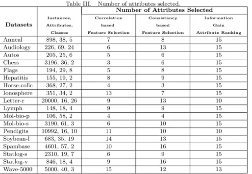
For each dataset belonging to Group 2, Table III shows the number of attributes selected by the early mentioned techniques. The number of attributes selected byCorrelation-based Feature Selection andConsistency-based Feature Selectiontechniques was automatically defined by their search method. ForInformation Gain Attribute Rankingtechnique, as the number of attributes is an input parameter, the value 15 was chosen for the majority of the datasets, and the values 10 or 13 for three datasets with larger number of instances.
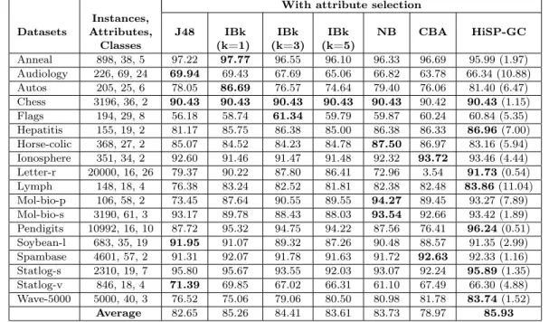
The experimental results for the datasets in Group 2 are presented in four tables: accuracy results for all classification techniques using datasets with attributes selected byCorrelation-based Feature Selection (Table IV), Consistency-based Feature Selection (Table VI), Information Gain Attribute Ranking (Table VIII), and accuracy results for all techniques (except for HiSP-GC) using original datasets, i.e., with no attribute selection (Table X).
Table III. Number of attributes selected.
Number of Attributes Selected
Instances, Correlation Consistency Information
Datasets Attributes, based based Gain
Classes Feature Selection Feature Selection Attribute Ranking
Anneal 898, 38, 5 7 8 15
Audiology 226, 69, 24 6 13 15
Autos 205, 25, 6 5 6 15
Chess 3196, 36, 2 3 6 15
Flags 194, 29, 8 5 8 15
Hepatitis 155, 19, 2 8 9 15
Horse-colic 368, 27, 2 4 3 15
Ionosphere 351, 34, 2 13 7 15
Letter-r 20000, 16, 26 9 13 10
Lymph 148, 18, 4 9 9 15
Mol-bio-p 106, 58, 2 4 4 15
Mol-bio-s 3190, 61, 3 6 10 15
Pendigits 10992, 16, 10 11 10 10
Soybean-l 683, 35, 19 14 13 15
Spambase 4601, 57, 2 10 16 15
Statlog-s 2310, 19, 7 6 9 15
Statlog-v 846, 18, 4 9 16 15
Wave-5000 5000, 40, 3 15 12 13
For Tables IV, VI and VIII, the datasets names are listed in the first column and their characteristics (number of instances, number of attributes and number of classes) are described in the second column. From third to eighth columns we observe the average accuracy results obtained with the algorithms J48, IBk (k=1), IBk(k=3), IBK (k=5), NB (Naive Bayes) and CBA, respectively. The last column presents the average accuracies for HiSP-GC and, in parentheses, the standard deviation for each average. In these tables, for each dataset, the largest accuracy value among those obtained by the methods included in the comparison is in bold font. The last row in these tables presents the average accuracy result for each technique.
The results presented in the last row of Table IV show that, on average, HiSP-GC reached the best accuracy (85.93%). The other algorithms ranked as follows, in descending order: IBk (K=1) (85.26%), IBk(K=3) (84.41%), NB (83.73%), IBk(K=5) (83.61%), J48 (82.65%) and CBA (78.97%).
Table V presents the results of the statistical analysis used to compare the predictive performance of HiSP-GC with the other techniques. In this case, all techniques used datasets with attributes selected byCorrelation-based Feature Selection method. Analyzing the results of this table, we can note that HiSP-GC always presents a number of better results greater than worse results. For example, when compared with decision tree technique (J48 column), HiSP-GC reached better results for 7 datasets, worse results for 2 datasets and equal results for 9 datasets.
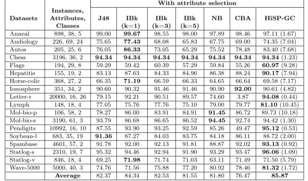
The results for all techniques using datasets with attributes selected byConsistency-based Feature Selection method are showed in Table VI. We can observe that, in the last row of this table, the average accuracy of HiSP-GC was better than those reached by the other classifiers. While HiSP-GC achieves accuracy of 85.87%, the other algorithms ranked as follows, in descending order: IBk(K=1) (84.34%), IBk(K=3) (82.53%), J48 (82.37%), NB (81.80%), IBk(K=5) (81.55%) and CBA (76.47%).
Table IV. Results for Group 2 (all techniques used the datasets reduced byCorrelation-based Feature Selection).
With attribute selection Instances,
Datasets Attributes, J48 IBk IBk IBk NB CBA HiSP-GC
Classes (k=1) (k=3) (k=5)
Anneal 898, 38, 5 97.22 97.77 96.55 96.10 96.33 96.69 95.99 (1.97) Audiology 226, 69, 24 69.94 69.43 67.69 65.06 66.82 63.78 66.34 (10.88) Autos 205, 25, 6 78.05 86.69 76.57 74.64 79.40 76.06 81.40 (6.47) Chess 3196, 36, 2 90.43 90.43 90.43 90.43 90.43 90.42 90.43(1.15) Flags 194, 29, 8 56.18 58.74 61.34 59.79 59.87 60.24 60.84 (5.35) Hepatitis 155, 19, 2 81.17 85.75 86.38 85.00 86.38 86.33 86.96(7.00) Horse-colic 368, 27, 2 85.07 84.52 84.23 84.78 87.50 86.97 83.16 (5.94) Ionosphere 351, 34, 2 92.60 91.46 91.47 91.48 92.32 93.72 93.46 (4.44) Letter-r 20000, 16, 26 79.37 90.22 87.80 86.41 72.96 3.54 91.73(0.54) Lymph 148, 18, 4 76.38 83.24 82.52 81.81 82.38 82.48 83.86(11.04) Mol-bio-p 106, 58, 2 73.45 87.64 90.55 89.55 94.27 89.45 93.27 (7.89) Mol-bio-s 3190, 61, 3 93.17 89.78 88.43 88.03 93.54 92.66 93.42 (1.89) Pendigits 10992, 16, 10 87.72 95.32 94.75 94.22 87.56 76.41 96.24(0.51) Soybean-l 683, 35, 19 91.95 91.07 89.32 87.26 90.48 88.57 91.35 (2.99) Spambase 4601, 57, 2 91.31 92.07 91.78 91.63 91.72 92.63 92.33 (1.16) Statlog-s 2310, 19, 7 95.80 95.67 93.55 92.03 93.07 92.24 95.89(1.35) Statlog-v 846, 18, 4 71.39 69.85 67.02 66.31 61.10 67.49 66.30 (4.88) Wave-5000 5000, 40, 3 76.52 75.06 79.06 80.50 80.98 81.78 83.74(1.52)
Average 82.65 85.26 84.41 83.61 83.73 78.97 85.93
Table V. Comparison between HiSP-GC and the other techniques (t-test results). IBk IBk IBk
J48 (k= 1) (k= 3) (k= 5) NB
Better Results 7 6 8 9 6
Worse Results 2 3 0 0 1
Equal Results 9 9 10 9 10
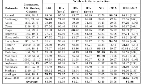
Finally, the accuracy results for the techniques using datasets with attributes selected by Informa-tion Gain Attribute Ranking method are presented in Table VIII. Similarly to the previous exper-iments, the average accuracy results presented in the last row of this table indicate the superiority of HiSP-GC when compared with the other classifiers. HiSP-GC reaches 86.88% and the other tech-niques ranked as follows, in descending order: IBk(K=1) (84.39%), IBk(K=3) (84.21%), IBk(K=5) (83.47%), J48 (83.36%), NB (82.46%) and CBA (75.96%).
Again, the results of statistical analysis, showed in Table IX, confirm that HiSP-GC, in terms of predictive accuracy, frequently performed better than the other techniques adopted in this work. For example, when compared with Naive Bayes classifier (NB column), HiSP-GC achieved better predictive accuracy for 11 datasets, worse for 1 dataset and equal for 6 datasets.
Although HiSP-GC, for datasets in Group 2, had been used only with datasets reduced by attribute selection techniques, for the other techniques the experiments were carried out with both original and reduced datasets. Therefore, Table X presents the accuracy results for all techniques (except for HiSP-GC) using original datasets, i.e., with no attribute selection. From third to eighth columns we observe the average accuracy results obtained with the algorithms J48, IBk (k=1), IBk (k=3), IBK (k=5), NB (Naive Bayes) and CBA, respectively, for the original datasets, without attribute selection. The last three columns show the average accuracy results for HiSP-GC with their respective standard deviation in parentheses, considering the datasets after attribute selection.
HiSP-Table VI. Results for Group 2 (all techniques used the datasets reduced byConsistency-based Feature Selection).
With attribute selection Instances,
Datasets Attributes, J48 IBk IBk IBk NB CBA HiSP-GC
Classes (k=1) (k=3) (k=5)
Anneal 898, 38, 5 99.00 99.67 98.55 98.00 97.89 98.46 97.11 (1.67) Audiology 226, 69, 24 75.65 77.43 68.08 65.83 67.75 69.00 74.35 (7.04) Autos 205, 25, 6 76.05 86.33 73.05 65.29 75.52 78.48 83.40 (7.68) Chess 3196, 36, 2 94.34 94.34 94.34 94.34 94.34 94.34 94.34(1.23) Flags 194, 29, 8 59.29 59.42 60.39 57.29 59.84 55.26 60.97(9.28) Hepatitis 155, 19, 2 83.13 87.63 84.33 84.96 86.38 88.24 90.17(7.94) Horse-colic 368, 27, 2 66.35 71.19 66.59 66.33 64.65 66.64 69.58 (7.17) Ionosphere 351, 34, 2 90.60 90.32 91.46 91.46 90.90 92.00 90.61 (4.82) Letter-r 20000, 16, 26 79.15 92.21 90.51 89.57 74.60 3.87 94.08(0.44) Lymph 148, 18, 4 77.05 75.76 77.76 75.10 79.00 79.77 81.10(10.45) Mol-bio-p 106, 58, 2 78.27 86.00 83.91 84.91 91.45 86.72 89.73 (10.18) Mol-bio-s 3190, 61, 3 93.79 86.68 86.65 86.52 94.45 92.74 94.42 (1.30) Pendigits 10992, 16, 10 87.55 93.90 93.25 92.59 85.26 49.47 95.12(0.53) Soybean-l 683, 35, 19 91.36 87.27 84.03 83.75 84.18 86.11 88.72 (2.00) Spambase 4601, 57, 2 91.78 92.00 92.13 91.81 88.87 92.02 93.13(0.92) Statlog-s 2310, 19, 7 95.32 94.46 92.94 91.90 93.29 93.47 96.06(1.09) Statlog-v 846, 18, 4 69.25 71.98 71.74 71.03 63.11 71.49 71.50 (5.79) Wave-5000 5000, 40, 3 74.76 71.56 75.88 77.20 80.92 78.46 81.32(1.72)
Average 82.37 84.34 82.53 81.55 81.80 76.47 85.87
Table VII. Comparison between HiSP-GC and each other techniques (t-test results). IBk IBk IBk
J48 (k= 1) (k= 3) (k= 5) NB
Better Results 7 6 9 10 9
Worse Results 2 2 0 0 0
Equal Results 9 10 9 8 9
GC reached average accuracy higher than the other classifiers (which used original datasets). While HiSP-GC reaches 85.93%, 85.87% and 86.88%, considering the datasets with attributes selected by Correlation-based Feature Selection, Consistency-based Feature Selection and Information Gain At-tribute Ranking, respectively, the other algorithms ranked as follows (in descending order): IBk(K=1) (84.38%), J48 (83.95%), IBk(K=3) (83.57%), IBk(K=5) (82.98%), NB (82.49%) and CBA (78.83%).
Table XI presents the results of statistical analysis. Now, the comparison was made between HiSP-GC (using datasets with attributes selected byCorrelation-based Feature Selection,Consistency-based Feature Selection and Information Gain Attribute Ranking) and each of the other techniques (us-ing original datasets, without attribute selection). The results obtained here were similar to those reported in the previous statistical analyses, that is, in terms of predictive accuracy, HiSP-GC was competitive and, frequently, better than other techniques used in these experiments. This can be verified, for example, by looking at IBk (K=5) column, where, regardless of the adopted attribute selection technique, HiSP-GC always achieves the best or equal accuracy for almost all datasets.
Table VIII. Results for Group 2 (all techniques used the datasets reduced byInformation Gain Attribute Ranking).
With attribute selection Instances,
Datasets Attributes, J48 IBk IBk IBk NB CBA HiSP-GC
Classes (k=1) (k=3) (k=5)
Anneal 898, 38, 5 98.00 95.20 93.67 96.89 92.76 98.68 98.11 (1.58) Audiology 226, 69, 24 75.24 74.28 69.78 65.43 68.56 72.14 72.55 (3.60) Autos 205, 25, 6 78.10 84.10 79.70 74.45 74.43 79.05 87.26(5.96) Chess 3196, 36, 2 97.09 96.46 93.81 95.46 89.61 96.70 95.87 (0.64) Flags 194, 29, 8 61.03 57.29 66.40 63.45 62.45 55.22 61.39 (7.10) Hepatitis 155, 19, 2 77.24 82.50 81.58 84.42 83.83 85.08 87.71(6.37) Horse-colic 368, 27, 2 87.70 79.91 82.67 81.57 83.96 79.67 82.91 (6.57) Ionosphere 351, 34, 2 91.21 93.45 91.17 91.17 91.74 94.56 93.45 (4.47) Letter-r 20000, 16, 26 79.40 90.89 88.48 87.21 73.33 3.54 92.65(0.61) Lymph 148, 18, 4 75.57 85.86 83.86 82.43 86.43 79.67 85.81 (10.23) Mol-bio-p 106, 58, 2 75.83 83.91 86.73 84.73 91.45 75.90 89.55 (8.39) Mol-bio-s 3190, 61, 3 91.89 83.35 85.33 85.67 95.80 94.56 95.11 (1.36) Pendigits 10992, 16, 10 86.78 91.94 91.58 90.97 82.18 29.07 93.55(0.40) Soybean-l 683, 35, 19 87.86 87.85 85.51 84.19 81.97 86.39 84.47 (2.93) Spambase 4601, 57, 2 91.52 91.65 91.98 91.89 91.11 92.53 92.94(0.88) Statlog-s 2310, 19, 7 95.32 93.12 92.64 92.08 91.26 93.10 94.76 (1.33) Statlog-v 846, 18, 4 73.74 71.07 71.04 69.50 62.05 69.96 72.09 (5.16) Wave-5000 5000, 40, 3 76.90 76.22 79.86 80.90 81.28 81.48 83.62(1.22)
Average 83.36 84.39 84.21 83.47 82.46 75.96 86.88
Table IX. Comparison between HiSP-GC and each other techniques (t-test results). IBk IBk IBk
J48 (k= 1) (k= 3) (k= 5) NB
Better Results 8 9 9 10 11
Worse Results 1 2 0 0 1
Equal Results 9 7 9 8 6
Table X. Results for Group 2 (only HiSP-GC used the datasets reduced by the attribute selection techniques). Instances, With no attribute selection With attribute selection
Datasets Attributes, J48 IBk IBk IBk NB CBA
Classes (k=1) (k=3) (k=5) HiSP-GC1 HiSP-GC2 HiSP-GC3 Anneal 898, 38, 5 98.78 99.22 97.89 96.77 94.88 98.01 95.99 (1.97) 97.11 (1.67) 98.11 (1.58) Audiology 226, 69, 24 78.75 71.25 60.95 58.70 66.80 70.75 66.34 (10.9) 74.35 (7.04) 72.55 (3.60) Autos 205, 25, 6 78.48 85.33 78.93 76.95 72.02 78.58 81.40 (6.47) 83.40 (7.68) 87.26 (5.96) Chess 3196, 36, 2 99.41 96.03 96.56 96.18 87.70 98.78 90.43 (1.15) 94.34 (1.23) 95.87 (0.64) Flags 194, 29, 8 62.53 56.74 57.87 61.47 60.89 57.27 60.84 (5.35) 60.97 (9.28) 61.39 (7.10) Hepatitis 155, 19, 2 76.00 83.08 86.96 84.96 84.54 81.87 86.96 (7.00) 90.17 (7.94) 87.71 (6.37) Horse-colic 368, 27, 2 86.96 77.70 75.83 74.22 81.80 81.87 83.16 (5.94) 69.58 (7.17) 82.91 (6.57) Ionosphere 351, 34, 2 90.02 93.17 90.61 89.19 90.31 93.72 93.46 (4.44) 90.61 (4.82) 93.45 (4.47) Letter-r 20000, 16, 26 78.85 91.78 90.42 89.86 74.02 3.87 91.73 (0.54) 94.08 (0.44) 92.65 (0.61) Lymph 148, 18, 4 76.33 85.19 82.48 82.43 85.76 79.01 83.86 (11.0) 81.10 (10.5) 85.81 (10.2) Mol-bio-p 106, 58, 2 75.36 82.18 83.00 79.09 89.64 71.90 93.27 (7.89) 89.73 (10.2) 89.55 (8.39) Mol-bio-s 3190, 61, 3 94.33 74.51 77.34 79.59 95.20 91.70 93.42 (1.89) 94.42 (1.30) 95.11 (1.36) Pendigits 10992, 16, 10 88.23 97.18 96.84 96.58 87.90 83.91 96.24 (0.51) 95.12 (0.53) 93.55 (0.40) Soybean-l 683, 35, 19 93.27 91.95 91.65 90.62 89.45 90.05 91.35 (2.99) 88.72 (2.00) 84.47 (2.93) Spambase 4601, 57, 2 93.18 92.89 93.15 93.22 90.24 93.34 92.33 (1.16) 93.13 (0.92) 92.94 (0.88) Statlog-s 2310, 19, 7 95.15 94.16 93.68 92.86 91.65 93.90 95.89 (1.35) 96.06 (1.09) 94.76 (1.33) Statlog-v 846, 18, 4 68.90 72.10 71.38 71.02 61.34 69.01 66.30 (4.88) 71.50 (5.79) 72.09 (5.16) Wave-5000 5000, 40, 3 76.62 74.30 78.70 79.86 80.72 81.34 83.74 (1.52) 81.32 (1.72) 83.62 (1.22)
Average 83.95 84.38 83.57 82.98 82.49 78.83 85.93 85.87 86.88 1
Correlation-based Feature Selection. 2Consistency-based Feature Selection. 3Information Gain Attribute Ranking.
4.2 Speed and Scalability
Table XI. Comparison between HiSP-GC and each other techniques (t-test results).
With no attribute selection
IBk IBk IBk
J48 (k= 1) (k= 3) (k= 5) NB
Better Results 5 4 6 7 9
HiSP-GC with Worse Results 5 4 5 3 1
Correlation-based Feature Selection Equal Results 8 10 7 8 8
Better Results 6 5 5 5 9
HiSP-GC with Worse Results 5 6 4 2 2
Consistency-based Feature Selection Equal Results 7 7 9 11 7
Better Results 8 4 7 10 11
HiSP-GC with Worse Results 3 3 3 2 1
Information Gain Attribute Ranking Equal Results 7 11 8 6 6
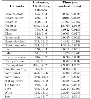
Due to its lazy approach, generally, HiSP-GC is slower than eager classifiers such as decision tree techniques. However, as can be observed in Tables XII and XIII, the average time spent by HiSP-GC to classify one instance was generally a small fraction of a second. In Table XII, we can observe that, for approximately 73% of datasets in Group 1, HiSP-GC spent, on average, less than one second to classify an instance. For only 9% of datasets, which are the largest (in number of attributes) in the Group 1, the classification time per instance exceeds three seconds.
Table XII. CPU time spent by HiSP-GC to classify one instance of Group 1.
Instances, Time (sec) Datasets Attributes, [Standard deviation]
Classes
Balance-scale 625, 4, 3 0.0067 [0.0026] Breast-cancer 286, 9, 2 0.0196 [0.0088] Breast-w 699, 9, 2 0.1663 [0.1382] Credit-a 690, 15, 2 1.8969 [1.0448] Diabetes 768, 8, 2 0.0842 [0.0185] Glass 214, 9, 6 0.0603 [0.0277] Hayes-roth 160, 4, 3 0.0045 [0.0023] Heart-cleveland 303, 13, 2 0.4942 [0.2199] Heart-hungarian 294, 13, 2 1.3219 [0.6639] Iris 150, 4, 3 0.0011 [0.0018] Labor 57, 16, 2 0.1978 [0.1263] Liver-disorders 345, 6, 2 0.0398 [0.0031] Postoperative 90, 8, 3 0.0062 [0.0032] Primary-tumor 339, 17, 21 7.9808 [4.2875] Shuttle-landing 15, 6, 2 0.0003 [0.0010] Solar-flare1 323, 12, 6 0.5506 [0.2356] Solar-flare2 1066, 12, 6 2.2314 [0.8965] Statlog-heart 270, 13, 2 0.8588 [0.3223] Tic-tac-toe 958, 9, 2 0.0351 [0.0044] Vote 435, 16, 2 4.2244 [3.1563] Wine 178, 13, 3 0.2994 [0.2955] Zoo 101, 17, 7 2.4613 [1.5613]
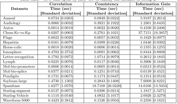
Although the datasets in Group 2 are larger than those pertaining to Group 1, after the size reduction obtained by the attribute selection techniques mentioned in Section 4.1, the classification time spent by HiSP-GC was as reduced as those presented for the datasets in Group 1. As can be observed in Table XIII, for all datasets reduced by theCorrelation-based Feature Selection, HiSP-GC spent, on average, less than two seconds to classify an instance. Being more specific, for 16 out of the 18 datasets, this classification time was only a fraction of a second.
col-Table XIII. CPU time spent by HiSP-GC to classify one instance of Group 2.
Correlation Consistency Information Gain
Datasets Time (sec) Time (sec) Time (sec)
[Standard deviation] [Standard deviation] [Standard deviation]
Anneal 0.0724 [0.0263] 0.0949 [0.0324] 5.9187 [3.2614] Audiology 0.0060 [0.0032] 0.3921 [0.1922] 1.2301 [0.8435] Autos 0.0014 [0.0019] 0.0022 [0.0020] 0.4100 [0.2406] Chess-Kr-vs-Kp 0.0207 [0.0063] 0.2761 [0.1021] 37.7151 [19.3857] Flags 0.0022 [0.0020] 0.0057 [0.0032] 0.1829 [0.0977] Hepatitis 0.0161 [0.0079] 0.0399 [0.0226] 1.0446 [0.9392] Horse-colic 0.0018 [0.0020] 0.0006 [0.0014] 0.1355 [0.1255] Ionosphere 0.4782 [0.3752] 0.0091 [0.0062] 0.8444 [0.8808] Letter-recognition 0.1792 [0.0972] 1.0714 [0.9979] 0.2612 [0.1845] Lymph 0.0225 [0.0076] 0.0117 [0.0046] 0.3906 [0.1649] Mol-bio-promoters 0.0006 [0.0014] 0.0005 [0.0014] 0.0313 [0.0524] Mol-bio-splice 0.0377 [0.0211] 0.1251 [0.0743] 0.6139 [0.4521] Pendigits 0.1731 [0.0675] 0.1174 [0.0447] 0.1314 [0.0518] Soybean-large 1.4730 [1.1302] 0.2843 [0.1408] 7.6009 [6.8221] Spambase 1.6277 [1.0570] 18.7108 [26.0220] 14.6166 [13.5034] Statlog-segment 0.0137 [0.0073] 0.0396 [0.0214] 1.1817 [1.5271] Statlog-Vehicle 0.1110 [0.0540] 4.0832 [3.1017] 2.6926 [2.3279] Waveform-5000 0.4423 [0.3812] 0.1526 [0.0504] 0.2356 [0.1821]
umn of Table XIII show that, for 15 out of the 18 datasets, HiSP-GC did not spend even a second to classify an instance. The exception was for Spambase, which even after the attribute reduction process, it remained with a large number of attributes and, therefore, the average classification time spent by HiSP-GC to classify an instance was superior to those presented by the remaining datasets in Group 2, reaching 18.7108 seconds. Finally, the results presented in the fourth column of Table XIII, concerning to the datasets reduced by Information Gain Attribute Ranking technique, show again that, for most datasets, HiSP-GC spent less than one second to classify an instance. Since the reduc-tion of these datasets was lower than the reducreduc-tion obtained byCorrelation-based Feature Selection andConsistency-based Feature Selection techniques, for Chess-Kr-vs-Kp andSpambase datasets, the average classification time per instance was superior to 10 seconds.
In order to analyze the scalability of HiSP-GC over the number of training instances we selected four datasets: Solar-flare2,Tic-tac-toe (the largest datasets in terms of number of instances of Group 1), Pendigits andLetter-recognition (the largest datasets in terms of number of instances of Group 2).
To examine the scalability of HiSP-GC, for each dataset, we randomly selected 90% of the original dataset as training instances and 10% as testing instances. Then, we formed four new training datasets using 20%, 40%, 60% and 80% of the training instances, all with the same number of attributes. Figure 2 shows the linear scalability of the average classification time per instance of HiSP-GC when the number of training instances increase inSolar-flare2,Tic-tac-toe,PendigitsandLetter-recognition. In this experiment, thePendigits and Letter-recognition datasets were reduced byCorrelation-based Feature Selectiontechnique.
5. CONCLUSION
An important challenge in data mining and machine learning areas is to build precise and computa-tionally efficient classifiers for different applications. In this work, we have proposed an instance-based classifier named HiSP-GC (HiSP General Classifier).
Fig. 2. Scalability on number of training instances.
on calculation ofa posterioriprobabilities, where the subsets of attribute values associated with larger probabilities of pertaining to some training class define the classification of the instanceX.
HiSP-GC was evaluated from experiments conducted on forty datasets from the UCI Machine Learning Repository. First, the predictive accuracy was the measure adopted for comparative tests among HiSP-GC and other traditional classifiers such as decision tree, k-Nearest Neighbor (k-NN), naive Bayes classifier and associative classifier. Our experimental results have shown that the accuracy achieved by HiSP-GC was better or similar to the accuracy obtained by the other methods.
Next, experiments were carried out to evaluate the performance of HiSP-GC with respect to compu-tational time and scalability over the number of training instances. Due to its classification approach, depending on the size of the dataset (number of attributes), HiSP-GC can present high computational costs to process it. Therefore, with the aim of making feasible the use of HiSP-GC for any size of dataset, in some cases, it was necessary a data preprocessing step to reduce the number of attributes in the dataset. Then, two groups of datasets were used in the experiments: one composed by datasets which were not reduced before being processed by HiSP-GC and other by datasets which were reduced before their processing. Our experimental results have shown that, for both groups of datasets, the average time spent by HiSP-GC to classify one instance was generally a small fraction of a second. This result confirms the usefulness of HiSP-GC for applications such as those present in this work. Also, the scalability tests showed that HiSP-GC is scalable over the number of training instances.
REFERENCES
Aha, D. W., editor. Lazy Learning. Springer, 1997.
Attwood, T. K.,Croning, M. D. R.,Flower, D. R.,Lewis, A. P.,Mabey, J. E.,Scordis, P.,Selley, J.,
and Wright, W.Prints-s: The database formerly known as prints. Nucleic Acids Research28 (1): 225–227, 2000.
Bateman, A.,Birney, E.,Durbin, R.,Eddy, S. R.,Howem, K. L.,and Sonnhammer, E. L. L. The pfam protein families database.Nucleic Acids Research 28 (1): 263–266, 2000.
Blake, C., Newman, D., Hettich, S., and Merz, C. UCI repository of machine learning databases. http://www.ics.uci.edu/∼mlearn/MLRepository.html, 1998. University of California, Irvine, Department of Infor-mation and Computer Sciences.
Cover, T. M. and Hart, P. E. Nearest neighbor pattern classification. IEEE Transactions on Information The-ory13 (1): 21–27, 1967.
Dayhoff, M. O. Establishing homologies in protein sequences.Methods in Enzymologyvol. 91, pp. 524–545, 1983.
Duda, R. and Hart, P. Pattern Classification and Scene Analysis. John Wiley & Sons, New York, 1973.
Fayyad, U. M. and Irani, K. B.Multi-interval discretization of continuous-valued attributes for classification learning. InProceedings of the International Joint Conference on Artificial Intelligence. Chambéry, France, pp. 1022–1029, 1993.
Garg, A. and Roth, D.Understanding probabilistic classifiers. Tech. Rep. UIUCDCSR-2001-2206, UIUC Computer Science Department. March, 2001.
Han, J. and Kamber, M. Data Mining: Concepts and Techniques. Morgan Kaufmann Publishers, New York, 2006.
Hatzidamianos, G.,Diplaris, S.,Athanasiadis, I.,and Mitkas, P. A.GenMiner: A data mining tool for protein analysis. InProceedings of the Panhellenic Conference On Informatics. Thessaloniki, Greece, pp. 346–360, 2003.
Haykin, S. Neural Networks: A Comprehensive Foundation. Macmillan Publishing Company, New York, 1994.
Henikoff, J. G.,Greene, E. A.,Pietrokovski, S.,and Henikoff, S. Increased coverage of protein families with the blocks database severs. Nucleic Acids Research28 (1): 228–230, 2000.
Henikoff, S. and Henikoff, J. G.Protein family databases. InEncyclopedia of life sciences. Macmillan Publishers Ltd, Nature Publishing Group, 2001. http://www.els.net.
Hulo, N.,Bairoch, A.,Bulliard, V.,Cerutti, L.,Castro, E. D.,Langendijk-Genevaux, P.,Pagni, M.,and Sigrist, C.The PROSITE database. Nucleic Acids Researchvol. 34, pp. 227–230, 2006.
Liu, B.,Hsu, W.,and Ma, Y. Integrating classification and association rule mining. InProceedings of the ACM SIGKDD International Conference on Knowledge Discovery and Data Mining. New York, USA, pp. 80–86, 1998.
Merschmann, L. and Plastino, A. A bayesian approach for protein classification. In Proceedings of the ACM Symposium on Applied Computing. Dijon, France, pp. 200–201, 2006a.
Merschmann, L. and Plastino, A. HiSP: A probabilistic data mining technique for protein classification. In
Proceedings of the International Workshop on Bioinformatics Research and Applications. LNCS 3992. Reading, U.K., pp. 863–870, 2006b.
Merschmann, L. and Plastino, A. A lazy data mining approach for protein classification. IEEE Transactions on Nanobioscience6 (1): 36–42, 2007.
Psomopoulos, F.,Diplaris, S.,and Mitkas, P. A.A finite state automata based technique for protein classification rules induction. InProceedings of the European Workshop on Data Mining and Text Mining in Bioinformatics. Pisa, Italy, pp. 54–60, 2004.
Quinlan, J. R.Induction of decision trees.Machine Learning 1 (1): 81–106, 1986.
Vapnik, V. N. The Nature of Statistical Learning Theory. Springer-Verlag, New York, 1995.
Veloso, A.,Meira Júnior, W., and Zaki, M. J. Lazy associative classification. In Proceedings of the IEEE International Conference on Data Mining. Hong Kong, China, pp. 645–654, 2006.
Wang, D.,Wang, X.,Honavar, V.,and Dobbs, D. L. Data-driven generation of decision trees for motif-based assignment of protein sequences to functional families. InProceedings of the Atlantic Symposium on Computational Biology, Genome Information Systems & Technology. North Carolina, USA, 2001.
Wang, J. T. L.,Zaki, M. J.,Toivonen, H. T. T.,and Shasha, D., editors. Data Mining in Bioinformatics. Springer, 2005.
Wang, X.,Schroeder, D.,Dobbs, D.,and Honavar, V. Automated data-driven discovery of motif-based protein function classifiers.Information Sciences 155 (1): 1–18, 2003.
Wang, Z. and Webb, G. I. Comparison of lazy bayesian rule and tree-augmented bayesian learning. InProceedings of the IEEE International Conference on Data Mining. Maebashi City, Japan, pp. 490–497, 2002.
Witten, I. H. and Frank, E.Data Mining: Practical Machine Learning Tools and Techniques with Java Implemen-tations. Morgan Kaufmann Publishers, San Francisco, 2005.