Comparison of methods for separating flood frequency of reservoir by sub-seasons

(1)

HESSD

12, 10431–10455, 2015

Methods for separating flood

frequency of reservoir by sub-seasons

J. Li et al.

Title Page

Abstract Introduction

Conclusions References

Tables Figures

◭ ◮

Back Close

Full Screen / Esc

Printer-friendly Version Interactive Discussion

Discussion

P

a

per

|

Discussion

P

a

per

|

Discussion

P

a

per

|

Discussion

P

a

per

Hydrol. Earth Syst. Sci. Discuss., 12, 10431–10455, 2015 www.hydrol-earth-syst-sci-discuss.net/12/10431/2015/ doi:10.5194/hessd-12-10431-2015

This discussion paper is/has been under review for the journal Hydrology and Earth System Sciences (HESS). Please refer to the corresponding final paper in HESS if available.

Comparison of methods for separating

flood frequency of reservoir by

sub-seasons

J. Li, M. Xie, K. Xie, and R. Li

School of Renewable Energy, North China Electric Power University, Beijing, China

Received: 1 September 2015 – Accepted: 22 September 2015 – Published: 14 October 2015

Correspondence to: J. Li (jqli6688@163.com, jqli6688@ncepu.edu.cn)

(2)

HESSD

12, 10431–10455, 2015

J. Li et al.

Title Page

Tables Figures

◭ ◮

Back Close

Full Screen / Esc

Discussion

P

a

per

|

Discussion

P

a

per

|

Discussion

P

a

per

|

Discussion

P

a

per

|

Abstract

The development of separate flood frequency distributions for different sub-seasons within a year can be useful for protection, storage and utilization of flood flows for the reservoir operation management. This paper applies conventional statistical method, fractal method and the mixed Von Mises distribution to the separation of flood

sub-5

seasons for inflows to Hongfeng Reservoir in China. Design floods are found for diff er-ent sub-seasons, along with flood control levels for flood regulation. The flood season is divided into four sub-seasons using the fractal method: the pre-rainy season (May), main-flood season (June and July), late-flood season I (August) and late-flood season II (September). The mixed Von Mises distribution method accounts for the general flood

10

pattern and combines August and September as one late-flood season, for three sub-seasons with different frequency distributions. The flood regulation calculation results show little difference between the control water levels in August and September, so the two can be combined into one period.

1 Introduction

15

Increasing water demands have intensified water scarcity in China. Reservoirs have a significant role in resolving the tension between the water supply and demand. To fully use flood resources and reduce water shortages, many researchers propose in-creased “floodwater utilization” (Cao, 2004). Floodwater utilization focuses on effective flood management through analyzing seasonal variation of floods with flood-control

20

safety, where reasonable separation of the flood season is a key for better benefit. Regulation for calculating design flood of water resources and hydropower projects of China requires that flood season separation should consider the design require-ments of projects, and have appropriate flood timing according to seasonal varying flood patterns. This means design floods of different sub-seasons should be calculated

25

(3)

oper-HESSD

12, 10431–10455, 2015

J. Li et al.

Title Page

Tables Figures

◭ ◮

Back Close

Full Screen / Esc

Discussion

P

a

per

|

Discussion

P

a

per

|

Discussion

P

a

per

|

Discussion

P

a

per

ation. Therefore, flood season separation is significant in calculating design floods of different stages and determining flood control levels, allowing better reservoir operation within different flood sub-seasons.

Flood operations of reservoirs are commonly for a single defined “flood season”, dif-fering from the remainder of the year when floods are unlikely to occur. Many methods

5

can help define the flood season, and to define how flood operations might vary in sub-seasons within the flood season. Many new methods also are available, such as fuzzy analysis, changing point analysis, fractal theory method etc. Chen (1995) proposed a fuzzy set application to flood season definition, reflecting fuzziness of flood season boundaries in time. The fuzzy membership functions used to separate flood season

10

and non-flood season are derived statistically, and the flood control level is calculated daily in the transition period to improve water utilization. Liu et al. (2005) introduced the theory of changing point analysis and detailed the theory and analytical method of mean changing point and probabilistic changing point in flood sub-seasons for the Three Gorges Reservoir. Hou et al. (1999) used fractal theory to analyze flood peak

15

sequence and studied flood sub-seasons for Xiaodeshi Station in China. The result of the fractal method is consistent with conventional empirical results. But the new method is less subjective. Fang et al. (2007) reviewed flood sub-season analysis methods and discussed their comparative advantages and disadvantages. Fang et al. (2008) used the Von Mises distribution as the annual maximum flood time distribution function to

de-20

scribe flood physical laws, and provided a new method for determining sub-seasonal design floods. Wei et al. (2014) used fractal theory in the study of flood sub-seasons for Bihe Reservoir. Because flood frequency distributions can be multimodal, Chen et al. (2010) used a mixed Von Mises distribution varying with flood date and derived sub-season varying design floods.

25

(4)

HESSD

12, 10431–10455, 2015

J. Li et al.

Title Page

Tables Figures

◭ ◮

Back Close

Full Screen / Esc

Discussion

P

a

per

|

Discussion

P

a

per

|

Discussion

P

a

per

|

Discussion

P

a

per

|

and flood control levels of different sub-seasons were then calculated according to the developed flood operating rules.

2 Methods of flood season separation

2.1 Statistical method – conventional method

To separate a flood season into sub-seasons, the physical cause of the flood should be

5

analyzed considering the meteorological and hydrologic characteristics of the studied river. Then according to the allocation pattern of rainfall and flood within a year and the inflow records of the representative hydrologic station, the flood frequency with given magnitude can be obtained. Generally, the physical cause of the flood and the hydro-logic characteristics of the river should be analysed first. According to the allocation

10

pattern of rainfall and flood and the inflow records for certain reservoir, the actual time and Cumulative probability of the first, second and third largest flood peaks of all the largest inflows occurring should be obtained under the time scale of month or ten day period. Next, based on the calculated frequencies, the separation of the flood season can be determined based on the seasonal changing pattern of the flood in combination

15

with the analysis of rainfall characteristic, storm characteristic, atmospheric circulation and other relevant meteorological factors.

2.2 Fractal theory method

2.2.1 Fractal theory

A fractal is a natural phenomenon or a mathematical set that has a repeating pattern

20

(5)

HESSD

12, 10431–10455, 2015

J. Li et al.

Title Page

Tables Figures

◭ ◮

Back Close

Full Screen / Esc

Discussion

P

a

per

|

Discussion

P

a

per

|

Discussion

P

a

per

|

Discussion

P

a

per

and water resources, such as the fractal of morphological characteristics of watershed systems, the longitudinal channel profile, and flood forecasting and flood disaster pre-diction (S. Zhang et al., 2009). J. Zhang et al. (2009) also have applied fractal theory to developing flood sub-seasons.

The current study of fractal is based on the qualitative understanding of the examined

5

object’s self-similarity. Whether the shapes measured byεbelong to the same fractal depends on whether the fractal dimension is fixed.

In physics and mathematics, the dimension of a mathematical space (or object) is informally defined as the minimum number of coordinates needed to specify any point within it. As for ordinary geometric shapes, points are 0-dimensional sets, lines are

10

1-dimensional sets which only have length, surfaces are 2-dimensional sets which have length and width, and cubes are 3-dimensional sets which have length, width and height. For complicated geometric forms whose details seem more important than the gross picture, fractal dimensions are applied as an index describing their complex-ity while the conventional Euclidean or topological dimension shows its limitation. If

15

the theoretical fractal dimension of a set exceeds its topological dimension, the set is considered to have fractal geometry (Mandelbrot, 2004). Unlike topological dimen-sions, the fractal index can take non-integer values (Sharifi-Viand et al., 2012). Multiple algorithms for calculating fractal dimension exist in fractal theory. The Hausdorff di-mension, also called gauge didi-mension, is the most basic. Others include information

20

dimension, correlation dimension, spectral dimension, distribution dimension and Lya-punov dimension, etc. The box-counting dimension (or Minkowski dimension) is used in this paper.

2.2.2 Calculation of box-counting dimension

Using a ruler of lengthεto measure a line segment of length L,N(ε) as the ratio of

25

(6)

HESSD

12, 10431–10455, 2015

J. Li et al.

Title Page

Tables Figures

◭ ◮

Back Close

Full Screen / Esc

Discussion

P

a

per

|

Discussion

P

a

per

|

Discussion

P

a

per

|

Discussion

P

a

per

|

this way is called box-counting dimension Dc (Zhu et al., 2011), and is defined as:

Dc= lim n→∞

lnN(ε)/ln(1/ε)

(1)

Whenεapproaches 0, it becomes:

lnN(ε)≈ −Dc lnε=Dc ln(1/ε) (2)

Whereε– the scale at which the fractal is measured, Dc – the box-counting dimension,

5

andN(ε) – the covering number.

If there is a straight part (clear correlation) on the lnNN(ε)−ln(ε) graph with linear fitting, the sequence can be conceived as a fractal. The slope of the straight part Dc is the fractal dimension. Smally (1987) introduced a new variable (NN) when computing the fractal dimension of the earthquake spectrum series of New Hebrides, namely the

10

relative measurement:

NN(ε)=N(ε)/NT (3)

Where N(ε) – absolute measurement, NT – total number of time intervals, T – total time length,ε– step length.

A fractal problem depends on the existence of a straight part (scale-invariant area)

15

on the lnNN(ε)−ln(ε) curve (Dong et al., 2007; Mandelbrot, 1983; Song et al., 2002; Ding et al., 1999). If the slope of the straight part in the scale-invariant area isb, the capacity dimension can be given by the following equation:

Dc=d−b (4)

Where d – topological dimension. Points of flood peaks distribute on a Q∼t

two-20

dimensional surface, sod equals to 2, and then:

(7)

HESSD

12, 10431–10455, 2015

J. Li et al.

Title Page

Tables Figures

◭ ◮

Back Close

Full Screen / Esc

Discussion

P

a

per

|

Discussion

P

a

per

|

Discussion

P

a

per

|

Discussion

P

a

per

2.3 Von Mises distribution method

2.3.1 Von Mises distribution

Compared with single normal distribution, the Von Mises distribution is a continuous probability distribution on a circle. This model primarily describes directional statistics. It is important in areas like astronomy, biology, geography, medicine, etc. For example,

5

He et al. (2011) applied the Von Mises yield criterion in the study of materials in plastic state in physics; Zheng et al. (2011) applied the Von Mises distribution model of monthly premium to analyze the seasonal fluctuation of the premium in medical science. The Von Mises distribution is also applied in hydrologic events. Fang et al. (2008) employed the Von Mises function to fit the time distribution of annual maximum flood and have

10

established a two-variable joint distribution of annual maximum flood.

The probability density curve of the Von Mises distribution is unimodal. However, the probability density curve of the time of the occurrence of floods in flood season also can be multimodal in practical calculation (Yue et al., 1999). Therefore, fitting result and actual measurement may differ when the Von Mises function is used to fit the probability

15

distribution of flood timing. Replacing the Von Mises distribution with mixed Von Mises distribution achieved well-fitted result (Chen et al., 2010).

2.3.2 Distribution establishment and parameter calculation

Assuming flood datet is normally distributed, its probability density function is (Fang et al., 2008):

20

f(t)= 1

2πI0(k)

exp [kcos (t−u)] 0≤t≤2π, 0≤u≤2π, k>0 (6)

(8)

HESSD

12, 10431–10455, 2015

J. Li et al.

Title Page Abstract Introduction Conclusions References Tables Figures ◭ ◮ ◭ ◮ Back Close

Full Screen / Esc

Printer-friendly Version Interactive Discussion Discussion P a per | Discussion P a per | Discussion P a per | Discussion P a per |

flood samples,Di – time of the occurrence of samplei, and:

a=

N

X

i=1

cosx_i/N b=

N

X

i=1

sinx_i/N (7)

wherex_i =D_i2π_L is the time of the occurrence of samplei (in radians), 0≺x_i≺2π. Thenuandk can be given by:

u=                   

arctanb/a a >0,b >0

2π+arctanb/a a >0,b <0

π+arctanb/a a <0

π/2 a=0,b >0

3π/2 a=0,b <0

indeterminate a=0,b=0

(8)

5

u=r=pa2₊_b2 ₀_≤_r _≤₁ ₍₉₎

In this study, the probability density function oftis given by:

f_t(t)=

n

X

i=1

pi

2πI₀(k_i)exp[kicos(t−ui)] 0≤t≤2π, 0≤ui ≤2π,k >0 (10)

Where n is the number of Von Mises distributions, p_i is the mixing percentage, and their optimal values that produce the best fitting result can be obtained with the

Quasi-10

Newton method (Li et al., 1997).

3 Application example

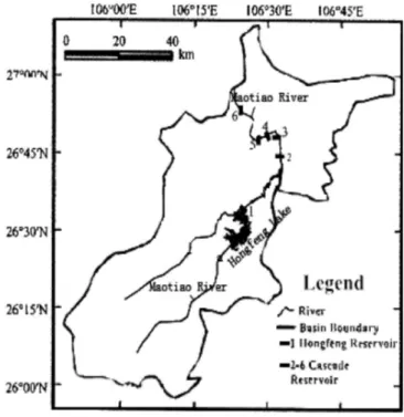
Built in 1960, Hongfeng reservoir is a large multi-year regulating storage reservoir for hydropower generation, flood control, water supply and recreation. As the lead-ing reservoir of the cascade of hydropower stations along Maotiao River, Hongfeng is

(9)

HESSD

12, 10431–10455, 2015

J. Li et al.

Title Page

Tables Figures

◭ ◮

Back Close

Full Screen / Esc

Discussion

P

a

per

|

Discussion

P

a

per

|

Discussion

P

a

per

|

Discussion

P

a

per

the key to ensuring the safety of the cascade system. The watershed controlled by Hongfeng reservoir has an area of 1596 km2, an average elevation of 1327 m, and an average river bed slope of 1.21 ‰. The Maotiao river flood season begins in May and ends in September, and rainfall in this period of time accounts for 70 % of annual in-flow. Annual maximum floods typically occur in June or July. The location of Hongfeng

5

Reservoir is shown in Fig. 1.

3.1 Flood season separation of Hongfeng reservoir

3.1.1 Application of statistical method

The flood season of Hongfeng reservoir is from 1 May to 30 September (lasting for 153 days). This study uses the historical hydrology record lasting 43 years.

10

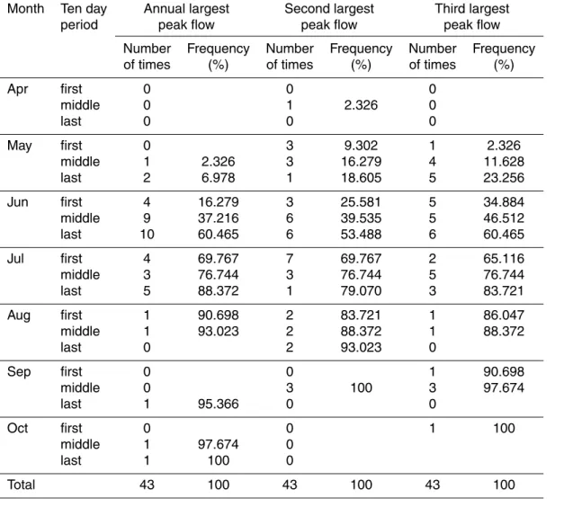
Table 1 shows that the largest flood within a year appears in the first ten day period of August, until the frequency of the largest inflow is 90.698 %, while the second and the third largest flood occur in the last ten day period of August and the first ten day period of September, until which the frequencies of the second and the third largest inflow are 93.023 and 90.698 % respectively during the whole flood record. In terms of

15

the multi-year average and largest inflow in a ten day period, the late July and the early August were at a low point as well as late August and early September. Therefore, the flood season of Hongfeng reservoir can be separated into three sub-seasons based on the analysis of its changing flood pattern and safety requirement. The pre-rainy season is from 1 May to 31 July, the middle flood season is from 1 August to 31 August, and

20

the late flood season is from 1 September to 30 September.

3.1.2 Application of fractal method

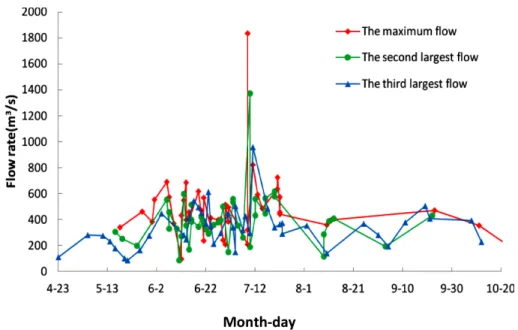
Earlier researches only sampled the sequence of the largest daily inflows, while this paper also accounts for the second and the third largest daily inflows. Distributions of the three largest daily inflows are shown in Fig. 2.

(10)

HESSD

12, 10431–10455, 2015

J. Li et al.

Title Page

Tables Figures

◭ ◮

Back Close

Full Screen / Esc

Discussion

P

a

per

|

Discussion

P

a

per

|

Discussion

P

a

per

|

Discussion

P

a

per

|

Figure 2 shows large gaps between the ten day period inflows of May and June, July and August, and August and September. So the flood season can be divided into four sub-seasons. Time scale ε is 1, 2, 3 ... 7, or 8 d. By setting a fixed value

Y1=235 m3s−1(slightly larger than the sample average inflow),N(ε) can be obtained under different time scales by counting the number of time intervals in which the

av-5

erage inflows exceedY1 (Fig. 3(1)). The lnNN(ε)−ln(ε) graph can be plotted to de-termine slope b of the straight part and then obtain the box-counting dimension Dc (Dc=2−b). Different lnNN(ε)−ln(ε) graphs can be plotted based on different values of T when changing the ending date of the first sub-season. Calculation of the lat-ter three sub-seasons is similar to the first sub-season, and the average inflows are

10

asY2₌540 m3s−1(Fig. 3(2)),Y3₌265 m3s−1(Fig. 3(3)),Y4₌235 m3s−1(Fig. 3(4)) respectively. The lnNN(ε)−ln(ε) graphs under different values of T of the four sub-seasons are shown in Fig. 3.

Shi et al. (2010) suggest that the significant linear relation between lnNN(ε) and ln(ε) is inversely proportional to the length of the time scale ε and thus should not

15

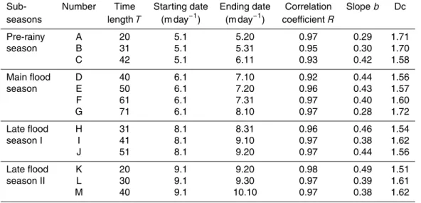
exceed 6. This case achieves the best result whenεis 8. The calculated box-counting dimensions of the four sub-seasons are shown in Table 2. From Table 2, the box-counting dimensions of situation A and situation B have a slight difference of 0.01 in the pre-rainy season, while situation C largely differs. According to the principle that the box-counting dimensions in the same sub-season should have similar magnitudes

20

while successive sub-seasons do not, A and B should belong to the same sub-season. So it can be concluded that the pre-rainy season is from 1 May to 31 May. Similarly, the box-counting dimensions of situation D, E and F are close with a relative di_fference less than 4 % in the main flood season, while G is rather different. So the main flood season is from 1 June to 31 July. In the late-flood season I, there is a discontinuous

25

(11)

HESSD

12, 10431–10455, 2015

J. Li et al.

Title Page

Tables Figures

◭ ◮

Back Close

Full Screen / Esc

Discussion

P

a

per

|

Discussion

P

a

per

|

Discussion

P

a

per

|

Discussion

P

a

per

the late-flood season I and the late-flood season II. In the late-flood season II, situation M is counted out because October is not included in the flood season. It can only be concluded that the late-flood season II is from 1 September to 20 September, and the remaining ten days until 30 September should be regarded as another sub-season if the fractal principle is strictly followed. However, to make it convenient for reservoir

5

management and operation, the late-flood season II should be from 1 September to 30 September.

The above separation was based on the sequence of the largest daily inflows. The separation results based on the sequences of the second and third largest daily in-flows are similar, which proves that taking sequence of only the largest daily inin-flows as

10

research sample is reasonable for separation.

3.1.3 Application of the mixed Von Mises distribution

Due to the scarce inflow records of Hongfeng reservoir, more reasonable flood peak records were adopted as samples to accurately trace changes in floods to make the distribution model more relevant. Based on Peaks-Over-Threshold (POT) sampling,

15

this study selected 156 Peaks-Over-Threshold (POT) floods from Hongfeng’s 43 year inflow records and two historical catastrophic floods in May 1830 and August 1892 with a threshold of 160 m3s−1. The selected sample floods satisfy the principles of independence and uniformity. A mixed Von Mises distribution with three parts (n=3) was then established. Relevant parameters areu1=0.50,k1=27.53,P1=0.10;u2=

20

(12)

HESSD

12, 10431–10455, 2015

J. Li et al.

Title Page

Tables Figures

◭ ◮

Back Close

Full Screen / Esc

Discussion

P

a

per

|

Discussion

P

a

per

|

Discussion

P

a

per

|

Discussion

P

a

per

|

the density function of this mixed Von Mises distribution are:

f1(t)= 1 2π×

0.10

6.89×10−10exp [27.53 cos (t−0.50)]

f2(t)= 1 2π×

0.66

4.22exp [2.82 cos (t−2.28)]

f3(t)= 1 2π×

0.24

5.10exp [3.05 cos (t−0.48)]

ft(t)=f1(t)+f2(t)+f3(t) (11)

5

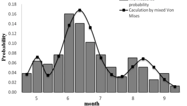
According to the above formulas, the fitting graph for the mixed Von Mises distribution of the floods occurring time is plotted in Fig. 4.

As shown in Fig. 4, floods in Maotiao River mainly occur in June and July and some-times in the middle of May, August and September. Floods in May, August and Septem-ber account for 16, 15 and 8 % respectively of all floods in flood season, while floods in

10

June and July are 61 % of all floods. The Maotiao River flood season is characterized with sub-seasons. In addition, the hydrologic records show that runoffin Maotiao River changes slightly from year to year but largely changes within one year. The largest annual flood generally occurs before August, mostly in June or July. Based on the selected sample sequence, two sub-season definitions were proposed. Both

strate-15

gies have May as the pre-rainy season, June and July as the main flood season. But one has August as the late-flood season I and September as the late-flood season II, while another combines August and September into one late-flood season. This paper shows that the theoretical curve based on the latter strategy can better fit the sample sequence, and apparently the mixed Von Mises distribution under such circumstance

20

(13)

HESSD

12, 10431–10455, 2015

J. Li et al.

Title Page

Tables Figures

◭ ◮

Back Close

Full Screen / Esc

Discussion

P

a

per

|

Discussion

P

a

per

|

Discussion

P

a

per

|

Discussion

P

a

per

3.2 Analysis on flood control levels of different sub-seasons for Hongfeng reservoir

According to Design Report of Cascade Hydropower Station in Maotiao River released in 1987 by the Ministry of water resources and Guiyang Engineering Corporation, the flood control level of Hongfeng reservoir was set at 1236.0 m, the highest reservoir

5

water level and the maximum discharge for the 100 yr design flood were 1239.97 m and 1420 m3s−1 respectively, and for the 5000 yr check flood were 1242.58 m and 2450 m3s−1respectively.

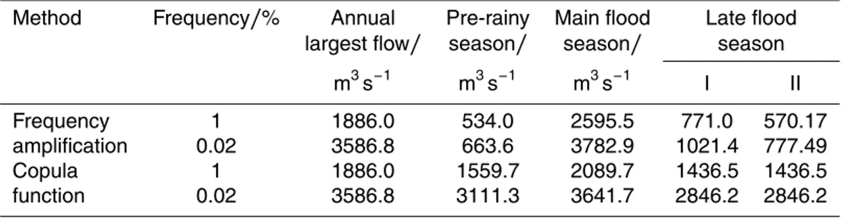
This paper used two new methods for developing flood sub-seasons and thus diff er-ent methods for design flood calculation. The fractal method used sampling of annual

10

largest values to calculate design floods of all sub-seasons by the same-frequency amplification method, while the mixed Von Mises distribution used POT sampling to establish the joint distribution of peak flow and occurring time of floods based on two-dimensional Frank Copula function to calculate the design floods. Peak flows of the 100 yr (1 % frequency) design flood and 5000 yr (0.02 % frequency) check flood of

dif-15

ferent sub-seasons from the above two methods are shown in Table 3.

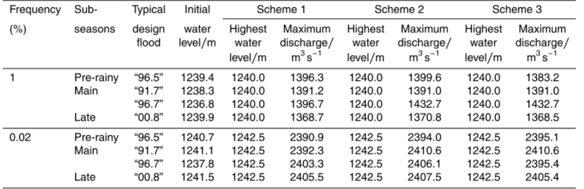
According to the separation result, this paper selected the flood in May 1996 for the pre-rainy season, two floods in July 1991 and July 1996 for the main flood season, the flood in August 2000 for the late-flood season I and the flood in September 1970 for the late-flood season II as typical sequence of floods. For the sub-seasons with the

20

mixed Von Mises distribution, flood in August 2000 was selected as a typical flood for the late-flood season. Three flood operating rules were applied to the design floods calculated from different typical floods, specifically open-discharge strategy, strategy for operating in 1987 and strategy for check in 1990. Operating results with the mixed Von Mises distribution sub-seasons are shown in Table 4.

25

(14)

HESSD

12, 10431–10455, 2015

J. Li et al.

Title Page

Tables Figures

◭ ◮

Back Close

Full Screen / Esc

Discussion

P

a

per

|

Discussion

P

a

per

|

Discussion

P

a

per

|

Discussion

P

a

per

|

For different design flood standards, the highest reservoir water levels from the above calculation are 1240.0 and 1242.58 m, and the largest discharge flows are 1420.0 and 2450.0 m3s−1.

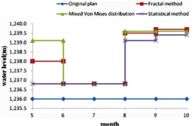
Flood control level changes with flood sub-seasons. Flood control levels in the pre-rainy season and the late-flood season are higher than that of the main flood season,

5

which increases the operating water level of Hongfeng reservoir in the whole flood season. In addition, the reservoir could release surplus water later and store more water for drought after the flood season. Due to the lack of data, calculating the design flood based on rainfall data was not carried out. For safety, this paper adjusted the calculated flood control levels and the final result is close to the research done by Li

10

(2007). Flood control levels of Hongfeng reservoir in di_fferent sub-seasons with three methods are shown in Fig. 5.

4 Conclusions

The aim of the separation of the flood season of certain reservoir is to determine more reasonable flood regulation schemes, which can make better use of the surplus water

15

and increase the full-guarantee rate of reservoirs in the flood season under the premise safety of hydraulic structure. So, the development of flood frequencies for sub-seasons within the annual flood season has potential to improve multipurpose reservoir system operation.

1. With long-term flood record, the conventional statistical method can be used for

20

flood season separation through frequency calculation. The fractal theory is ap-plicable to flood series featured with randomness, nonlinearity, determinacy and similarity. In this paper, by using the first three largest sequences of daily inflow as research samples for the fractal method, so it only revealed statistics of ex-treme values. A POT (Peaks-Over-Threshold sampling) method was used to

se-25

(15)

HESSD

12, 10431–10455, 2015

J. Li et al.

Title Page

Tables Figures

◭ ◮

Back Close

Full Screen / Esc

Discussion

P

a

per

|

Discussion

P

a

per

|

Discussion

P

a

per

|

Discussion

P

a

per

independence of flood sample and makes up for short flood records. Therefore, results based on POT method can reflect the rules of flood occurrence.

2. On the whole, the separation results from the fractal theory and mixed Von Mises distribution are similar to the conventional method. As reservoir operation be-comes more difficult with more flood sub-seasons, the mixed Von Mises

distribu-5

tion method achieves a more reasonable result.

Acknowledgements. This study was financially supported by the CRSRI Open Research Pro-gram (ProPro-gram SN: CKWV2015232/KY) and National Natural Science Foundation of China (No. 41340022). There are special thanks to Professor Jay R. Lund and Hui Rui from University of California, Davis who gave many helpful comments on this paper.

10

References

Cao, Y.: Study on floodwater utilization and management, Resour. Ind., 6, 21–23, 2004. Chen, L., Guo, S., Yan, B., and Liu, P.: A new seasonal design flood estimation method, Engin. J.

Wuhan Univ., 43, 20–24, 2010.

Chen, S.: Methodology of fuzzy sets analysis to hydrologic system from research on flood

15

period description, Adv. Water Sci., 6, 133–138, 1995.

Ding, J. and Liu, G.: Estimation of fractal dimension for daily flow hydrograph, Si Chuan Water Power, 18, 74–76, 1999.

Dong, Q., Wang, X., Wang, J., and Fu, C.: Application of fractal theory in the stage analysis of flood seasons in Three Gorges Reservoir, Resour. Environ. Yangtze Basin, 16, 400–404,

20

2007.

Fang, B., Guo, S., Liu, P., and Xiao, Y.: Advance and assessment of seasonal design flood methods, J. Hydroelectr. Power, 33, 71–75, 2007.

Fang, B., Guo, S., Xiao, Y., Liu, P., and Wu, J.: Annual maximum flood occurrence dates and magnitudes frequency analysis based on bivariate joint distribution, Adv. Water Sci., 19,

25

505–511, 2008.

(16)

HESSD

12, 10431–10455, 2015

J. Li et al.

Title Page

Tables Figures

◭ ◮

Back Close

Full Screen / Esc

Discussion

P

a

per

|

Discussion

P

a

per

|

Discussion

P

a

per

|

Discussion

P

a

per

|

Hou, Y., Wu, B., and Zheng, G.: Preliminary study on the seasonal period’s classification of floods by using fractal theory, Adv. Water Sci., 10, 140–143, 1999.

Li, J., Ji, C., Lu, Q., and Li, A.: Flood control limited level of Hongfeng reservoir during the former flood season, J. North China Electric Power Univ., 34, 27–31, 2007.

Li, Y.: The Direction of Statistics, China Science and Technology Publishing House, Beijing (in

5

Chinese), 129–131, 1997.

Liu, P., Guo, S., and Wang, C.: Flood season staged for three gorges reservoir based on the change-point approach, Hydrology, 25, 18–23, 2005.

Liu, Y., Hu, M., Yu, G., and Li, X.: Theory of fractal and its applications, Jiang Xi Sci., 24, 205–209, 2006.

10

Mandelbrot, B. B.: The Fractal Geometry of Nature, Freeman, San Francisco, 1983. Mandelbrot, B. B.: Fractals and Chaos, Springer, Berlin, 32, xii, 308, 2004.

Sharifi-Viand, A., Mahjani, M. G., and Jafarian, M.: Investigation of anomalous di_ffusion and

multifractal dimensions in polypyrrole film, J. Electroanal. Chem., 671, 51–57, 2012.

Shi, Y., Li, M., and Zheng, Y.: Flood season staged in Xiangjiang river basin based on fractal

15

theory, B. Soil Water Conserv., 30, 165–167, 2010.

Smally, R. F.: A fractal approach to the clustering of earth quakes: application to the simplify of the New Hebrides, BSSA , 27, 32–49, l987.

Song, L.: Analyses on sudden change in low tide level series of the Caoe River, J. Sediment Res., 1, 69–71, 2002.

20

Wei, W., Mo, C., Liu, L., Jiang, Q., Sun, G., and Jiang, H.: Application of watershed rainfall fractal theory in reservoir flood season staging, Yellow River, 36, 39–41, 2014.

Yue, S., Ouarda, T. B. M. J., Bobe’e, B., Legendre, P., and Bruneau, P.: The Gumbel mixed model for flood frequency analysis, J. Hydrol., 88–100, 1999.

Zhang, J., Huang, Q., Ma, Y., and Wang, Y.: Division of flood seasonal phases for reservoir and

25

the evaluation method, J. Northwest A&F University (Nat. Sci. Ed.), 37, 229–234, 2009 Zhang, S., Wang, W., Ding, J., and Chang, F.: Application of fractal theory to hydrology and

water resources, Adv. Water Sci., 16, 141–146, 2009.

Zheng, Y., Zhang, J., and Yang, H.: Application of Von Mises distribution in insurance premium in Shaanxi Province, Stat. Inform. Forum, 26, 28–30, 2011.

30

(17)

HESSD

12, 10431–10455, 2015

J. Li et al.

Title Page

Tables Figures

◭ ◮

Back Close

Full Screen / Esc

Discussion

P

a

per

|

Discussion

P

a

per

|

Discussion

P

a

per

|

Discussion

P

a

per

Table 1.Frequency of the occurence of the first three largest peak flows.

Month Ten day Annual largest Second largest Third largest

period peak flow peak flow peak flow

Number Frequency Number Frequency Number Frequency

of times (%) of times (%) of times (%)

Apr first 0 0 0

middle 0 1 2.326 0

last 0 0 0

May first 0 3 9.302 1 2.326

middle 1 2.326 3 16.279 4 11.628

last 2 6.978 1 18.605 5 23.256

Jun first 4 16.279 3 25.581 5 34.884

middle 9 37.216 6 39.535 5 46.512

last 10 60.465 6 53.488 6 60.465

Jul first 4 69.767 7 69.767 2 65.116

middle 3 76.744 3 76.744 5 76.744

last 5 88.372 1 79.070 3 83.721

Aug first 1 90.698 2 83.721 1 86.047

middle 1 93.023 2 88.372 1 88.372

last 0 2 93.023 0

Sep first 0 0 1 90.698

middle 0 3 100 3 97.674

last 1 95.366 0 0

Oct first 0 0 1 100

middle 1 97.674 0

last 1 100 0

(18)

HESSD

12, 10431–10455, 2015

J. Li et al.

Title Page

Tables Figures

◭ ◮

Back Close

Full Screen / Esc

Discussion

P

a

per

|

Discussion

P

a

per

|

Discussion

P

a

per

|

Discussion

P

a

per

|

Table 2.Box-counting dimensions of different flood sub-seasons.

Sub- Number Time Starting date Ending date Correlation Slopeb Dc

seasons lengthT (m day−1) (m day−1) coefficientR

Pre-rainy A 20 5.1 5.20 0.97 0.29 1.71

season B 31 5.1 5.31 0.95 0.30 1.70

C 42 5.1 6.11 0.93 0.42 1.58

Main flood D 40 6.1 7.10 0.92 0.44 1.56

season E 50 6.1 7.20 0.96 0.43 1.57

F 61 6.1 7.31 0.97 0.40 1.60

G 71 6.1 8.10 0.97 0.28 1.72

Late flood H 31 8.1 8.31 0.96 0.46 1.54

season I I 41 8.1 9.10 0.97 0.38 1.62

J 51 8.1 9.20 0.97 0.44 1.56

Late flood K 20 9.1 9.20 0.98 0.49 1.51

season II L 30 9.1 9.30 0.97 0.39 1.61

(19)

HESSD

12, 10431–10455, 2015

J. Li et al.

Title Page

Tables Figures

◭ ◮

Back Close

Full Screen / Esc

Discussion

P

a

per

|

Discussion

P

a

per

|

Discussion

P

a

per

|

Discussion

P

a

per

Table 3.Peak flows of design floods of different sub-seasons.

Method Frequency/% Annual Pre-rainy Main flood Late flood

largest flow/ season/ season/ season

m3s−1 m3s−1 m3s−1 I II

Frequency 1 1886.0 534.0 2595.5 771.0 570.17

amplification 0.02 3586.8 663.6 3782.9 1021.4 777.49

Copula 1 1886.0 1559.7 2089.7 1436.5 1436.5

(20)

HESSD

12, 10431–10455, 2015

J. Li et al.

Title Page

Tables Figures

◭ ◮

Back Close

Full Screen / Esc

Discussion

P

a

per

|

Discussion

P

a

per

|

Discussion

P

a

per

|

Discussion

P

a

per

|

Table 4.Results of flood regulation.

Frequency Sub- Typical Initial Scheme 1 Scheme 2 Scheme 3 (%) seasons design water Highest Maximum Highest Maximum Highest Maximum

(21)

HESSD

12, 10431–10455, 2015

J. Li et al.

Title Page

Tables Figures

◭ ◮

Back Close

Full Screen / Esc

Discussion

P

a

per

|

Discussion

P

a

per

|

Discussion

P

a

per

|

Discussion

P

a

per

(22)

HESSD

12, 10431–10455, 2015

J. Li et al.

Title Page

Tables Figures

◭ ◮

Back Close

Full Screen / Esc

Discussion

P

a

per

|

Discussion

P

a

per

|

Discussion

P

a

per

|

Discussion

P

a

per

|

(23)

HESSD

12, 10431–10455, 2015

J. Li et al.

Title Page

Tables Figures

◭ ◮

Back Close

Full Screen / Esc

Discussion

P

a

per

|

Discussion

P

a

per

|

Discussion

P

a

per

|

Discussion

P

a

per

(1)Y1=235m3/s (2) Y2=540m3/s

(3) Y3=265m3/s (4) Y4=235m3/s

(24)

HESSD

12, 10431–10455, 2015

J. Li et al.

Title Page

Tables Figures

◭ ◮

Back Close

Full Screen / Esc

Discussion

P

a

per

|

Discussion

P

a

per

|

Discussion

P

a

per

|

Discussion

P

a

per

|

(25)

HESSD

12, 10431–10455, 2015

J. Li et al.

Title Page

Tables Figures

◭ ◮

Back Close

Full Screen / Esc

Discussion

P

a

per

|

Discussion

P

a

per

|

Discussion

P

a

per

|

Discussion

P

a

per