www.hydrol-earth-syst-sci.net/18/4325/2014/ doi:10.5194/hess-18-4325-2014
© Author(s) 2014. CC Attribution 3.0 License.
Variational assimilation of remotely sensed flood extents using
a 2-D flood model
X. Lai1, Q. Liang2, H. Yesou3, and S. Daillet4
1State Key Laboratory of Lake Science and Environment, Nanjing Institute of Geography & Limnology, CAS, Nanjing 210008 P.R. China
2School of Civil Engineering and Geosciences, Newcastle University, Newcastle upon Tyne, NE1 7RU, UK 3SERTIT, Université de Strasbourg, Bd Sébastien Brant, BP 10413 67412 Illkirch, France
4LEGOS/CNES, 18 avenue Edouard Belin, 31401 Toulouse, CEDEX 9, France Correspondence to:X. Lai ([email protected])
Received: 5 June 2014 – Published in Hydrol. Earth Syst. Sci. Discuss.: 26 June 2014 Revised: 5 September 2014 – Accepted: 19 September 2014 – Published: 4 November 2014
Abstract.A variational data assimilation (4D-Var) method is proposed to directly assimilate flood extents into a 2-D dy-namic flood model to explore a novel way of utilizing the rich source of remotely sensed data available from satellite imagery for better analyzing or predicting flood routing pro-cesses. For this purpose, a new cost function is specially defined to effectively fuse the hydraulic information that is implicitly indicated in flood extents. The potential of us-ing remotely sensed flood extents for improvus-ing the analysis of flood routing processes is demonstrated by applying the present new data assimilation approach to both idealized and realistic numerical experiments.
1 Introduction
Flooding poses a significant threat to human society. Nowa-days, floods are becoming more frequent as a result of in-tensive regional human activities and environmental change. Hydraulic or hydrodynamic models have become reliable and cost-effective tools to analyze and predict flood rout-ing through catchments, rivers, and floodplains. These mod-els can provide dynamic outputs (e.g., inundation area, wa-ter depth, and/or flow velocity) for flood warning and risk assessment. Nevertheless, models are not perfect, and un-certainties and computational errors may arise from various sources, including the uncertainties associated with hydro-logical parameters, initial and boundary conditions, as well as numerical errors as a result of numerical discretization
and mathematical approximations (Le Dimet et al., 2009; Pappenberger et al., 2007a). In order to reduce prediction er-rors or uncertainties, field measurements are usually used to verify and calibrate a model before applying it to make pre-dictions. Traditional trial and error approaches are commonly used in model calibration, but they are known for being sub-jective and tedious (Ding, 2004). Therefore, in order to make a better prediction, it would be more beneficial to have more intelligent calibration methods achieved by fusing a dynamic flood model with observed information to obtain an optimal estimate of model states and parameters.
In river hydraulics, the available measurements commonly include water stage (level) and discharge at hydrological sta-tions, and velocity at gauging points. These measurements are generally sparse, even for those study areas with decent monitoring systems, and are therefore likely to be insufficient to support reliable model calibration. During a flood event, the available measurements may be even scarcer due to mal-functioned operation of some monitoring systems under ex-treme flow conditions and the difficulty in performing field surveys. Fortunately, rich sources of remote sensing data with different spatial and temporal coverage now become increas-ingly available. Remote sensing imagery provides spatially distributed information about flood states, which is hard to obtain from the traditional point-based field-measuring ap-proaches (Hostache et al., 2010). As a whole, due to their low cost and large coverage, remotely sensed data are now be-coming an important source of measurements, and they are widely applied to flood monitoring and loss evaluation for flood hazards (Pender and Néelz, 2007). Furthermore, recent intensive research – such as the direct estimation of hydraulic variables (e.g., flow discharge and water stage) from satellite imagery, the use of remote sensing data to calibrate and val-idate models, the fusion of these data with dynamic models using data assimilation methods, among others – has signif-icantly contributed to the advances of integrating remotely sensed data from space with flood models (e.g., Schumann et al., 2009; Smith, 1997).
Substantial efforts have been made using the 4D-Var and Bayesian-updating methods to demonstrate the potential of assimilating remotely sensed data from space for improv-ing flood prediction (Andreadis et al., 2007; Durand et al., 2008; Giustarini et al., 2011; Komma et al., 2008). Roux and Dartus (2006) attempted to determine flood discharge from a remotely sensed river width using a 1-D hydraulic model. In 2-D river hydraulic modeling, 4D-Var methods have been developed to assimilate spatially distributed wa-ter stage (Lai and Monnier, 2009) and Lagrangian-type ob-servations; e.g., remotely sensed surface velocity (Honnorat et al., 2009, 2010). Hostache et al. (2010) employed a 4D-Var method to assimilate the water stage derived from a RADARSAT-1 image of the 1997 Mosel River flood event in France into a 2-D flood model to improve model calibration. Water stage can be indirectly derived from satellite imagery or directly measured by satellite altimetry. The accuracy of indirect water stage retrieval from satellite imagery is typi-cally in a range of 40–50 cm (Alsdorf et al., 2007; Hostache et al., 2010; Matgen et al., 2010). Simple overlay analysis of a Digital Elevation Model (DEM) and a flood-extent map may lead to high errors on the order of meters, even when a 30 m resolution ERS ASAR (Advanced Synthetic Aperture Radar) image is used (Brakenridge et al., 1998; Oberstadler et al., 1997; Schumann et al., 2011). Generally, additional steps must be performed in order to obtain an acceptable es-timation of water levels for using with hydrodynamic mod-eling. The complexity of these steps varies with the
meth-ods being applied (Matgen et al., 2007, 2010; Raclot, 2006; Schumann et al., 2007). For instance, Raclot (2006) and Hostache et al. (2010) used a hydraulic coherence constraint to minimize the estimation errors. Schumann et al. (2007) proposed a Regression and Elevation-based Flood Informa-tion eXtracInforma-tion model (REFIX) for water depth estimaInforma-tion and later suggested an alternative for deriving water level from river cross-section data (Schumann et al., 2008). There-fore, the derivation of water level from flood extent with ac-ceptable accuracy is not a straightforward procedure.
Inland water level can also be directly measured from satellite altimetry that is originally developed for open oceans. The database of altimetric water level for about 250 sites on large rivers in the world has been developed based on satellite altimetry missions (http://www.legos.obs-mip.fr/en/ soa/hydrologie/hydroweb/). For oceans and great lakes, the accuracy of estimating water level may reach a few centime-ters (Fu and Cazenave, 2001; Crétaux and Birkett, 2006). For rivers and floodplains, the retrieved water level data quality is highly variable (Santos da Silva et al., 2010), most typically at 50 cm (Alsdorf et al., 2007). However, despite its relative high accuracy for large inland water bodies, compared with the indirectly retrieved water level, the present in-orbit satel-lite altimetry (four satelsatel-lites includingSaral/AltiKa, Jason-2, HY-2, and Cryosat-2) is still problematic because of the spa-tial and temporal resolutions and coverage for sampling rela-tive small water bodies. It essentially provides only spot mea-surements of water level (Alsdorf et al., 2007). To improve this, an exciting satellite mission called the Surface Water and Ocean Topography (SWOT) using swath-based technol-ogy has been proposed and will be launched for accurate monitoring of inland water bodies (https://directory.eoportal. org/web/eoportal/satellite-missions/s/swot). The SWOT mis-sion provides great potential and new opportunity for data collection in the near future (in 2020). However, currently, the rich optical and Synthetic Aperture Radar (SAR) images will still be the main sources of remote sensing data for mon-itoring floods. Therefore, it is still of great interest to inves-tigate the combined assimilation of the currently available multi-source satellite data.
In contrast to water stage, the remotely sensed flood ex-tent can be directly derived from satellite imagery without affecting the original resolution (for example, 30 m for En-visat ASAR and 250 m for MODIS data), which is compa-rable to the mesh size normally adopted in flood modeling. Various simple and mature approaches are available for rapid and automatic extraction of a flood-extent map from optical and SAR imageries (Matgen et al., 2011; Smith, 1997). How-ever, to the best of our knowledge, there has been no attempt at the direct assimilation of flood-extent data into a 2-D dy-namic flood model using a 4D-Var method to date.
function is specifically constructed to effectively fuse the hy-draulic information available implicitly in flood extents. The numerical results show that the proposed 4D-Var method can effectively assimilate the flood-extent data and improve the prediction accuracy of flood routing. The rest of the paper is organized as follows. First, a short description is given in Sect. 2 to introduce the 2-D flood model coupled with a 4D-Var method. In order to implement the assimilation of the observed flood extent into the 2-D flood model, Sect. 3 pro-poses a cost function that measures the discrepancy between observed data and modeling results. The new approach is val-idated by idealized tests in Sect. 4, before being applied to a realistic case in Sect. 5. Finally, a summary and brief conclu-sions are drawn in Sect. 6.
2 The 2-D dynamic flood model with variational data assimilation
2.1 Overview of variational data assimilation
4D-Var is a method based on the optimal control theory of a physical system governed by partial differential equations (Le Dimet and Talagrand, 1986). It allows us to perform flow state analysis or prediction of a system by combining a physi-cally based dynamic model with observations. To implement a 4D-Var, a cost function must firstly be defined to measure the discrepancy between the computational results and ob-servations. The cost function J over the time interval from t=0 tot=T without regularization terms may be given as
J (p)=1
2
T
Z
0
kHU−Ok2dt ,
=1
2
T
Z
0
(HU−O)TW−1(HU−O)dt , (1)
wherepis the control vector,k·kis the Euclidean norm,H is the observation operator that maps the space of the state variables to the space of observations,Uis the vector of state variables,Wis the error covariance matrix, andOis the ob-served data. Herein, the statistical information can be incor-porated into the norm through the error covariance matrixW. 4D-Var can be considered as an unconstrained optimiza-tion problem that seeks an optimal control vectorp∗to min-imize the cost functionJ (p)in Eq. (1). According to the
op-timal control theory, optimum conditions are reached if the gradientJ=0, which means that an optimal control vector
is obtained and the optimal flow analysis results are closest to the true (measured) state. This optimization problem may be solved by a descent-type algorithm, and the quasi-Newton minimization subroutine M1QN3, developed by Gilbert and Lemaréchal (1989), is adopted in this work. The algorithm calculates the gradient of the cost function – i.e., the vector
of its partial derivatives with respect to each of the control variables –, which may be efficiently performed using the adjoint method, as described in Sect. 2.3.
2.2 2-D shallow water equations
The 2-D SWEs are widely used to approximate flood routing over a floodplain. They can be written in a conservative form as follows:
∂U ∂t +
∂F(U)
∂x +
∂G(U)
∂y =B(U) , (2)
wherex andy represent the Cartesian coordinates,t is the
time,U=(h, hu, hv)T=(h, qx, qy)Tis a vector containing
the flow variables, withhbeing the water depth anduandv
the two velocity components,F=(hu, hu2+0.5gh2, huv)T
andG =(hv, huv, hv2+0.5gh2)T are the flux vectors in
the x and y directions, g is the gravitational acceleration, B = [0, gh(S0x-Sf x),gh(S0y−Sf y)]T is the vector of the
source terms,S0x= −∂Zb/∂xandS0y = −∂Zb/∂yare the two bottom slopes, withZbdenoting the bed elevation, and Sf x=n2qxh−7/3
q
qx2+qy2andSf y=n2qyh−7/3
q qx2+qy2
are the two friction slopes inxandydirections, respectively,
withnbeing the Manning roughness coefficient. Given
ini-tial and boundary conditions, the flood routing process over a floodplain may be numerically predicted on different tem-poral and spatial scales by solving the above governing equa-tions.
2.3 Adjoint governing equations
The adjoint method, based on an optimal control theory (Le Dimet and Talagrand, 1986), is usually applied to compute the gradient of the cost function, owing to its computational burden, independent of the dimension of problems (Cacuci, 2003). The adjoint equations for the 2-D SWEs can be de-rived for the cost function in Eq. (1), as follows:
∂U∗ ∂t +
∂F ∂U
T∂U∗
∂x + ∂G ∂U
T∂U∗
∂y =−
∂B ∂U T
U∗
+HTW(O−HU), (3)
where the adjoint variableU∗=(h∗, qx∗, qy∗)Tand the
coeffi-cient matrices are given by
∂F ∂U T
=
0 −u2+c2 −uv
1 2u v
0 0 u
,
∂G ∂U T
=
0 −uv −v2+c2
0 v 0
1 u 2v
,
∂BT ∂U =
0 gS0x+73gSf x gS0y+73gSf y
0 −gSf x 2u
2+v2
u(u2+v2) −gSf y
u
u2+v2
0 −gSf xu2+vv2 −gSf y u
2+2v2
v(u2+v2)
The partial derivative of the cost functionJ corresponding
to the control vector p is a simple function of the adjoint variablesU∗, which can be found in Lai and Monnier (2009). Adopting the adjoint equations in gradient computation significantly reduces the computational cost because evalu-ation of the adjoint variables requires only one backward in-tegral in time. Once the adjoint variables are known, the par-tial derivatives of the cost function with respect to the control variables can be computed in a straightforward way. 2.4 Forward model and adjoint model
The 2-D SWEs in Eq. (2) are discretized using a finite vol-ume Godunov-type scheme with the inter-cell mass and mo-mentum fluxes evaluated using the HLLC (Harten-Lax-van Leer-Contact) approximate Riemann solver (Toro, 2001). The scheme has first-order accuracy in space but provides high-resolution representation of flow discontinuities. Time discretization is achieved using an explicit Euler scheme. Readers may consult Honnorat et al. (2007) for a more de-tailed description of the shallow flow model, which is re-ferred to as the “forward model” herein.
The adjoint model is developed by directly differentiating the source codes of the forward model that solve the 2-D SWEs in Eq. (2). The automatic differentiation tool TAPE-NADE (Hascoët and Pascual, 2004) is adopted in this work to generate the reverse codes. This method, based on source codes, helps to build a consistent adjoint model correspond-ing to the forward solver.
3 Cost function for flood-extent assimilation
As mentioned previously in the introduction, the flood ex-tent can be derived from satellite imagery more directly and easily than the water stage. However, the flood extent is not a state variable in the 2-D SWEs, but basically the union of pixels, where water depth is not 0. Therefore, it has no ex-plicit relationship to the state variables. As a consequence, it is difficult to define a cost function to implement the as-similation of flood extent in the framework of 4D-Var. In this work, we implement the assimilation of flood-extent infor-mation into a 2-D dynamic flood model through an implicit way.
If we assume a functionf as an observable quantity, the
cost function may be defined as
J (p)=1
2
T
Z
0
f−f
obs
2
dt , (4)
in which, the regularization terms are neglected from the above cost function to facilitate simplified but more infor-mative verification and validation of the proposed method, and they allow direct investigation of the potential benefit of assimilating flood-extent data.
To determine the cost function for assimilation of the hydraulic information, including implicitly in the remotely sensed flood-extent data, a specific form off should be
in-troduced. Here, we define the flood extent related quantity
f as a function with regard to state variables of water,U, namely
f (U)=A(h)U, (5)
whereAis a matrix with regard to water depth that describes the wet–dry status, namely flood-extent information.
Normally, the wet–dry status of a computational cell can be determined by its water depth,h. It is dry if water depth
is 0; otherwise, it is wet. However, a finite threshold (critical value) of water depth,hc, must be defined at water
bound-ary in real-world problems. This is essential to minimize the effects of the disturbances from different land covers, the res-olution of the image, and other sources of uncertainty, as suggested by Aronica et al. (2002). It should be noted that the matrix,A, describing the wet–dry status of the computa-tional cells, should be determined according to the difference between the predicted water depth andhcso as to keep the
consistence with the observed flood-extent data derived from imagery. The matrixAcan be simply obtained as
A(h)=
a11 0 . . . 0
0 a22 . . . 0 . . . .. . . .
0 0 . . . ann
, (6)
in which
aii=
1
, h≥hc
0, h < hc
.
The above expression shows that the matrixAdynamically changes with the flood routing.
For the flood-extent observation derived from satellite im-ages, the matrixAobs infobs is an error matrix of
observa-tion describing wet–dry status informaobserva-tion. It should be de-termined by the specific method for extracting flood extent.
Aobs(h)=
a11 a12 . . . a1n
a21 a22 . . . a2n
. . . .. . . . an1 an2 . . . ann
(7)
If solely error variances are considered,Aobscan be simpli-fied as follows:
Aobs(h)=
a11 0 . . . 0
0 a22 . . . 0 . . . .. . . .
0 0 . . . ann
Ω ,1J =1 0.5 2
(1-w h)2 Ω ,
2
2
J =2 0.5w(-h)
2 w=0
hc
w=1 0< <1w
Ω1
Ω2
Completely dry,w=0
Completely wet,w=1
Predicted wet area
Partially wet (uncertainty), 0<w<1
Possible active cells during assimilation True flood front
(water boundary line)
(a) (b)
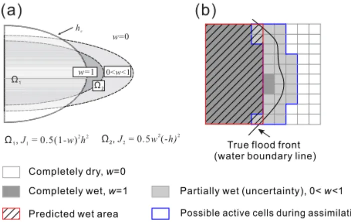
Figure 1. Definition of a cost function. (a) The concept map; (b)grid-based map for showing the specific definition of cost func-tion and possible active cells during data assimilafunc-tion.
in which,aiirepresents the wet–dry status or the degree of
certainty of a pixel being wet in a remotely sensed image. Uncertainty in the observed flood extent can be determined by, e.g., using the fuzzy set approach (Pappenberger et al., 2007b). In the positions with high uncertainty, aii will be
assigned by a very low certainty degree. Low certainty lets the extent information in these positions take little effect on the estimate of flood states.
A normalized weight, w (ranging from 0 to 1), is
intro-duced in this work to describe this certainty. As shown in Fig. 1, w=1 indicates a pixel being definitely wet, and
w=0 denotes a pixel being absolutely dry. The value in
be-tween is given according to the level of certainty of a pixel being wet. The observed flood-extent map can then be de-picted in a 2-D raster format with pixel values equal to w
(Fig. 1). When observations are used, they should be mapped into the model space by an observation operator.
Assumingf =Ah, whereU=h, we can interpretf as a
physically meaningful variable; i.e., a unit water volume. In a view that the weightw inArepresents the certainty of a cell being wet, deriving from observations but not the cer-tainty of observed water depth, it is better to be used to con-strain the discrepancy of predicted and observed water depth when defining cost function. For those overlapping regions between the predicted and observed extents, no discrepancy information should be used for assimilation and the corre-sponding cells should be deactivated in the computation of cost function, because the predicted wet–dry status is always the same as the observed one. Considering that, we further modified the cost function to become
J (p)=0.5X
t(h−h
obs)T(A−Aobs)T
(A−Aobs)(h−hobs). (9)
The remaining difficulty is to determine the observed water depth. To overcome this, the computational domain is first separated into two parts, as illustrated in Fig. 1; i.e.,1 repre-sents the region with predicted water depthh > hc, while2
is the area outside of1. In either part, the observed water
depth is assumed to be identical to the prediction when com-puting cost function if the wet–dry status of the computed cell is the same as the observation belonging to the same flood extent. It should be noted that this assumption excludes those cells in the overlapping regions between the predicted and observed extents from the computation of cost function. In those non-overlapping regions, different assumptions have to be made, depending on the specific location under consid-eration. Inside1, the observed water depth is defined to be
“0” if the cell under consideration is outside the area cov-ered by the remotely sensed flood extent. As a result, the cost function in1may be defined asJ1=0.5(1−w)2h2, where wis the certainty of flooding, as described in the previous
paragraph. Obviously,J1decreases to 0 when the predicted and observed extents coincide. Inside2, an observed water
depth,hobs, is required to construct the cost function in those
areas covered by the remotely sensed flood extent. Numerical experiments show that it is feasible to sethobs=2hto keep
a similar gradient along the boundary, which leads to a cost functionJ2=0.5w2(–h)2in2.J2 will also decrease to 0 when the predicted and observed extents coincide. Although this assumption seems to be “unrealistic”, it is mathemati-cally reasonable in the computation of cost function, and it is effective for assimilating flood extent to drive the assimi-lation algorithm.
Taking into account all of above considerations, the cost function measuring the discrepancy of observations and pre-dictions over computational domain may be written as
J (p)=0.5X
t
X
1(1−wi)
2h2
i
+X
2w
2
i(−hi)2
. (10)
4 Test cases
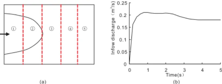
4.1 Dyke-break flood routing over a flat bottom We first consider a flood routing process induced by a dyke break over a 10 m×8 m rectangular floodplain with a flat
bottom (i.e.,Zb=0). As shown in Fig. 2a, the left boundary
represents a river bank with a breach of 0.4 m in the middle. The floodplain consists of five types of land covers corre-sponding to Manning’sn: 0.03, 0.04, 0.05, 0.06, and 0.07,
respectively, from left to right. The computational domain has been discretized into a uniform mesh of a 0.2 m×0.2 m
resolution. During the simulation, a fixed time step of 0.01 s is used. The boundary discharge hydrographQi(t )(half of
total discharge through dyke breach to floodplain) is shown in Fig. 2b and imposed on each of the two breach cells. The other three lateral boundaries of the floodplain are assumed to be solid walls. The floodplain is initially dry.
With the aforementioned “accurate”n set for each land
0 0.05 0.1 0.15 0.2 0.25
0 1 2 3 4 5
Time(s)
Infow
d
ischarge
m
/s)
(
3
○1 ○2 ○3 ○4 ○5
(a) (b)
Figure 2.Idealized test of flood routing over a rectangular flood-plain induced by dyke breach:(a)computational domain;(b) hy-drograph of the inflow dischargeQi(t ).
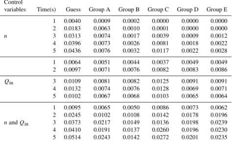
Table 1.The five groups of observations used in the test case of dyke-break flood routing over a flat bottom.
Description of observations
Group A Flood extent att=5 s
Group B Flood extents att=1, 3, and 5 s
Group C Z(t ), time history of water stage at central position of floodplain (time interval of measurement is 0.2 s) Group D Flood extent att=5 s andZ(t )
Group E Flood extents att=1, 3, and 5s andZ(t )
by the forward model for 5 s over the floodplain. Synthetic binary maps of the flood extent and the time history of water stage in the middle of the domain are generated and will be used as observed data during the following numerical exper-iments. Five groups of observations are obtained, as listed in Table 1, with different combinations of synthetic flood ex-tents and/or the stage hydrograph at the central point. The assimilation window is set to be 5 s (the same as the duration of the forward simulation). Three series of numerical experi-ments are carried out by controllingn,Qi(t ), or both of them,
respectively.
In this case, a series of numerical experiments are carried out to verify the model using the accurate synthetic data gen-erated that can eliminate the disturbances of numerical and measured errors encountered in an actual case.
4.1.1 Experiment series A
The control variable of the experiment series A is the dis-tributed Manning coefficient n. Five assimilation
experi-ments are run with the same first guess ofn0=0.02 over the
whole floodplain, but with different groups of synthetic data being assimilated. In each run, the optimal analysis of flood routing over the floodplain is undertaken and the distributed
nis retrieved, as provided in Table 2.
Table 3 lists the root-mean-square (RMS) errors of water depth over the whole computational domain at different out-put times. For the runs involving the observations of groups A and B, which just assimilate flood extents, the RMS errors decrease by 78 and 94 %, respectively. This is also clearly
Table 2.The identified Manning’snin experiment series A and C.
Observations 1 2 3 4 5
True value – 0.03 0.04 0.05 0.06 0.07
First guess – 0.02
Series A
Group A 0.031 0.053 0.053 0.028 0.042 Group B 0.030 0.038 0.054 0.036 0.074 Group C 0.030 0.040 0.050 0.020 0.020 Group D 0.030 0.040 0.050 0.042 0.070 Group E 0.030 0.04 0.05 0.038 0.072
Series C
Group A 0.024 0.061 0.118 0.099 0.220 Group B 0.031 0.069 0.057 0.032 0.046 Group C 0.020 0.052 0.040 0.020 0.020 Group D 0.052 0.047 0.052 0.039 0.049 Group E 0.047 0.077 0.026 0.023 0.030
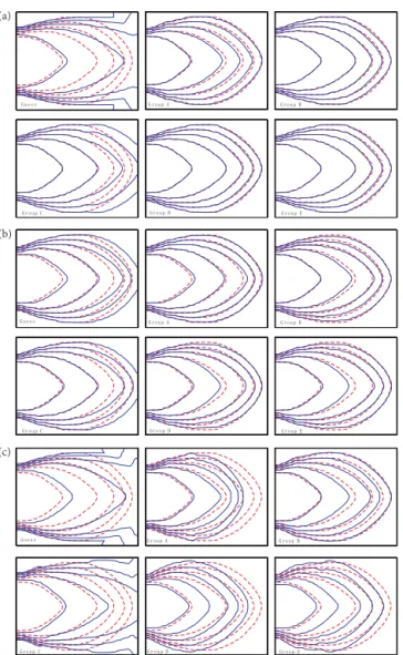
demonstrated by comparing the flood extents obtained from different runs that assimilate different observations (Fig. 3a). After data assimilation, the predicted flood extents are sig-nificantly improved and agree much more closely with the “observed” extents. The more observed flood-extent data are assimilated, the closer the results become to the “true” state. In the numerical experiment involving water stage observa-tions (group C), only the stage hydrograph is assimilated, and the RMS errors decrease by 82 % on average. However, the predicted results att=3–5 s are significantly different to the
true states, which can also be seen evidently due to the differ-ence between the predicted and ‘true’ flood extents (Fig. 3a). The results from simulations using observations from groups D and E show that the RMS errors are further decreased by about 95 % after assimilating both the time series of water stage and spatial flood extents.
As a whole, by assimilating different synthetic data, dif-ferent levels of improvement in flood prediction have been achieved during the numerical experiments, which lead to the assimilated predictions that are always much closer to the true state. It confirms that the current assimilation analy-sis of fusing observed flood extent and relevant information improves the accuracy of flood prediction in both space and time (Fig. 5a). The quality of the assimilated results can also be confirmed from the identifiedn, as listed in Table 2. The
value of n for the first land block can be accurately
iden-tified in all of the experiments, regardless of whether flood extent or stage hydrograph is assimilated. However, since the stage hydrograph only provides upstream information, it can-not optimize the values ofnfor the downstream land blocks 4
and 5. Therefore, thenvalues remain to be their initial guess
in the numerical experiment using the group C observations, which leads to apparent difference between the simulated and true extents aftert=3–5 s (Fig. 3a).
4.1.2 Experiment series B
Table 3.The RMS errors of water depth att=1, 2, 3, 4, and 5 s in experiment series A, B, and C.
Control
variables Time(s) Guess Group A Group B Group C Group D Group E
1 0.0040 0.0009 0.0002 0.0000 0.0000 0.0000
2 0.0183 0.0063 0.0010 0.0001 0.0000 0.0000
n 3 0.0313 0.0074 0.0017 0.0039 0.0009 0.0012
4 0.0396 0.0073 0.0026 0.0081 0.0018 0.0022
5 0.0436 0.0076 0.0032 0.0117 0.0022 0.0028
1 0.0064 0.0051 0.0044 0.0037 0.0049 0.0049
2 0.0097 0.0071 0.0076 0.0082 0.0083 0.0086
Qin 3 0.0109 0.0081 0.0082 0.0125 0.0091 0.0091
4 0.0132 0.0074 0.0076 0.0128 0.0069 0.0071
5 0.0102 0.0067 0.0068 0.0103 0.0065 0.0064
1 0.0095 0.0065 0.0050 0.0086 0.0073 0.0062
2 0.0245 0.0102 0.0108 0.0142 0.0178 0.0196
nandQin 3 0.0373 0.0217 0.0149 0.0136 0.0198 0.0239
4 0.0410 0.0191 0.0137 0.0260 0.0196 0.0230
5 0.0514 0.0243 0.0142 0.0272 0.0201 0.0235
groups of observations. The initial guesses of discharge cal-culated byQ0i =Qi(1+0.6R), withRbeing a random
num-ber between 0 and 1, are imposed through the inflow bound-ary. With the help of the minimization algorithm, the initial guesses of the discharge boundary condition are corrected and the corresponding analysis results after data assimila-tion are computed. The hydrographs of inflow discharge for numerical experiments using the groups B, C, and E obser-vations are shown in Fig. 4a. They are slightly corrected to minimize the cost function.
The RMS errors of each run att=1, 2, 3, 4, and 5 s are
listed in Table 3. They decrease by 28∼32 % for those
sim-ulations assimilating the flood extents, but only 5 % for runs just assimilating point-based data provided as the stage hy-drograph. Figure 3b compares the predicted and true flood extents.
In this experiment series, it is interesting to note that better prediction over the whole duration and spatial extent (Table 3 and Fig. 3b) is produced by assimilating flood extent, even though poor prediction of water stage hydrograph at the cen-tral gauge station is found (Fig. 5b). Assimilation of these data can help to estimate the inflow hydrograph and then increase the assimilation accuracy. On the contrary, point-based time series data only imply part of the inflow discharge information prior to the propagation time from the inlet to the given points. The inclusion of point-based measurements helps to improve the accuracy of the stage hydrograph at the central station but has no obvious benefit for prediction for the whole duration and spatial extent.
4.1.3 Experiment series C
In the experiment series C, both the Manning coefficient and the inflow discharge hydrograph are controlled. The same initial guesses ofnand discharge are used. After running the
assimilation model,Qi(t )and the distributednare corrected
to minimize the cost function. Although the discharge hydro-graph (Fig. 4b) andn(Table 2) of each run are not well
iden-tified, the predictions (Fig. 3c) obtained after assimilating the flood extents are much closer to the true one than those just assimilating point-based measurements. The RMS errors of the runs assimilating the observations of group A, B, C, D, and E decrease by 50, 64, 45, 48, and 41 %, respectively, as listed in Table 3. It is encouraging to observe that almost half of the RMS errors decrease for each run. As in the exper-iment series B, although the inclusion of point-based mea-surements improves the accuracy of the stage hydrograph at the central station, no obvious improvement is detected in terms of overall RMS errors.
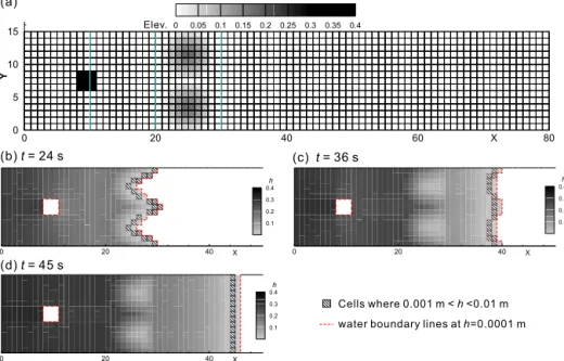
4.2 Flood routing over a complex bottom
A test case involving flood routing over three mounds are selected to further verify the performance of the proposed model under complex circumstances, which is similar to the previous cases (Begnudelli and Sanders, 2007). The chan-nel in this case has a length of 80 m and a width of 15 m (Fig. 6). Three mounds inside the channel are centered at (x, y)=(9.5, 7.5), (25, 3.5), and (25, 11.5), respectively. The
first mound at (9.5, 7.5) is a square island with an eleva-tion of 2 m. The second and third mounds at (25, 3.5) and (25, 11.5) are conidial with a height of 0.2 m and their eleva-tion is assumed to decrease linearly along the radial distance from the center at a rate of 1 : 4. The computational domain is discretized into a uniform mesh of a 1 m×1 m
resolu-tion. The channel bed is initially dry. Cases with both lumped and distributed bed roughness are investigated, respectively. A constant Manning’sn=0.03 is set up for the cases with
G u e s s
G r o u p C
G r o u p A
G r o u p D
G r o u p B
G r o u p E
G u e s s
G r o u p C
G r o u p A
G r o u p D
G r o u p B
G r o u p E
G u e s s
G r o u p C
G r o u p A
G r o u p D
G r o u p B
G r o u p E (a)
(b)
(c)
Figure 3. Comparison of the predicted and true flood extents at
t=1, 2, 3, 4, and 5 s for different simulations using guessed Man-ning’snand by assimilating the observations of group A, B, C, D, and E:(a)experiment series A;(b)experiment series B; and(c) ex-periment series C. The solid and dashed lines mark, respectively, the predicted and true flood extents.
when 10 m< x≤20 m, 0.03 when 20 m< x≤30 m, and
0.02 whenx >30 m. The steady unit discharge of 0.2 m2s−1
is imposed atx=0. The dyke-break flood routing is firstly
simulated by the forward model for 45 s using a fixed time step of 0.05 s. The assimilation window is set to be 45 s (the same as the duration of the forward simulation). Synthetic flood-extent data used in the assimilation are generated based on the simulated results.
In this test case, a number of numerical experiments are carried out to verify the use of the proposed method un-der complex circumstances. By using different water depth thresholds –hcfor determining observed flood extent –, the model independence on the selection of the thresholds is first
(a) True
Initial guess Group BGroup C Group E
Time(s)
is
arg
e(m
s)
(b) True
Initial guess Group BGroup C Group E
Figure 4.Identified discharge hydrograph from(a)experiment se-ries B and(b)experiment series C.
validated. Then, the influences of the uncertainties in flood-extent data on the assimilation results are examined.
4.2.1 Independence on water depth threshold
To validate the independence of assimilation on the selection of water depth threshold, the numerical experiments with a lumped (constant) roughness are conducted. Based on the simulated flood process using a lumped Manning’sn=0.03,
we generate the observed flood extents at t=24, 36, and
45 s using different water depth thresholds; i.e.,hc=0.0001,
0.001, and 0.01 m. By controlling the lumped Manning’s
n, the flood extents are assimilated into the flood dynamic
model. The unknown (or guessed) Manning’s coefficients are successfully identified after assimilation of a single flood extent at different times. The RMS errors of water depth (RMSEh)decrease significantly in all cases after the
assim-ilation of the given single flood-extent data (Fig. 7 and Ta-ble 4) although the Manning’s coefficients are not well iden-tified in the case that assimilates the flood extent att=24 s
whenhc=0.0001 m. These results indicate that the
assimila-tion performance and accuracy are not sensitive to the selec-tion of water depth threshold in the current method, provided it is in a reasonable range. It should note that water depth threshold is a finite magnitude that presents water depth of water boundary in real-world problems. Thus, the threshold cannot select arbitrarily, but it keeps the value as close to real water depth at water boundary line as possible. Sensitivity analysis may be conducted if required.
4.2.2 Influence of flood-extent uncertainty
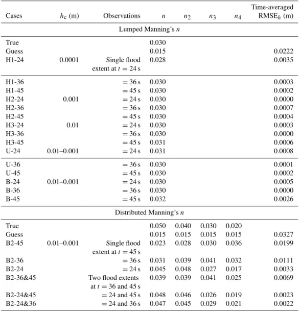
Table 4.The water depth threshold,hc, the assimilated observations, identified Manning’sn, and time-averaged RMS errors of water depth (RMSEh)in the test case of dyke-break flood routing over three mounds.
Time-averaged
Cases hc(m) Observations n n2 n3 n4 RMSEh(m)
Lumped Manning’sn
True 0.030
Guess 0.015 0.0222
H1-24 0.0001 Single flood 0.028 0.0035
extent att=24 s
H1-36 =36 s 0.030 0.0003
H1-45 =45 s 0.030 0.0002
H2-24 0.001 =24 s 0.030 0.0000
H2-36 =36 s 0.030 0.0007
H2-45 =45 s 0.030 0.0004
H3-24 0.01 =24 s 0.030 0.0003
H3-36 =36 s 0.030 0.0000
H3-45 =45 s 0.031 0.0006
U-24 0.01–0.001 =24 s 0.031 0.0008
U-36 =36 s 0.030 0.0001
U-45 =45 s 0.030 0.0002
B-24 0.01–0.001 =24 s 0.030 0.0005
B-36 =36 s 0.030 0.0000
B-45 =45 s 0.032 0.0026
Distributed Manning’sn
True 0.050 0.040 0.030 0.020
Guess 0.015 0.015 0.015 0.015 0.0327
B2-45 0.01–0.001 Single flood 0.023 0.028 0.030 0.036 0.0199
extent att=45 s
B2-36 =36 s 0.031 0.039 0.041 0.032 0.0111
B2-24 =24 s 0.045 0.048 0.027 0.017 0.0033
B2-36&45 Two flood extents 0.039 0.039 0.041 0.025 0.0069
att=36 and 45 s
B2-24&45 =24 and 45 s 0.048 0.046 0.026 0.019 0.0023
B2-24&36 =24 and 36 s 0.047 0.045 0.029 0.021 0.0022
uncertainty is tested. We assume that the flood areas are com-pletely wet ifh >0.01 m, completely dry ifh <0.001 m, and
partially wet or dry if 0.001 m< h <0.01 m. Therefore, the
weight or certainty degree of the cell being wet,wover whole
flood areas, can be determined byw=max (min ((max (h,
0.001)–0.001)/(0.01–0.001), 1), 0). This results in a grid-based flood-extent map for assimilation experiments.
Two groups of assimilation experiments with respectively lumped and distributed bed roughness are conducted. For the cases with lumped bed roughness, the accurate weights cal-culated from water depth are first used in our assimilation experiments (Case U-24, U-36, and U-45, as presented in Table 4). The successfully identified Manning’s n and the
decrease of near 99 % in RMSEh (Fig. 7 and Table 4) show
that the flood-extent uncertainty can be correctly accounted for in our proposed method. In realistic problems, the ideal weight is almost impossible to be accurately obtained. That
considered, more challenging cases are designed to verify the method (Case B-24, B-36, and B-45, as presented in Table 4). In these three experiments,wis assumed to be 0.5 for areas
with uncertainty (0.001 m< h <0.01 m). After assimilating
the given single flood extent, the controllingnis again
suc-cessfully identified, which leads to a dramatic decrease in RMSEh(Fig. 7 and Table 4).
Furthermore, the cases with distributed bed roughness are also considered (Case B2-24, B2-36, B2-45, B2-36&45, B2-24&45, and B2-24&36). We still use the observations with inaccurate weight, namely w=0.5 in areas with
0.001 m< h <0.01 m. After assimilating the given single
flood extent, the RMSEh in each experiment is apparently
reduced, although the true distributed Manning’sn cannot
be achieved for these cases (Table 4). However, when new observations are available, the RMSEh can decrease
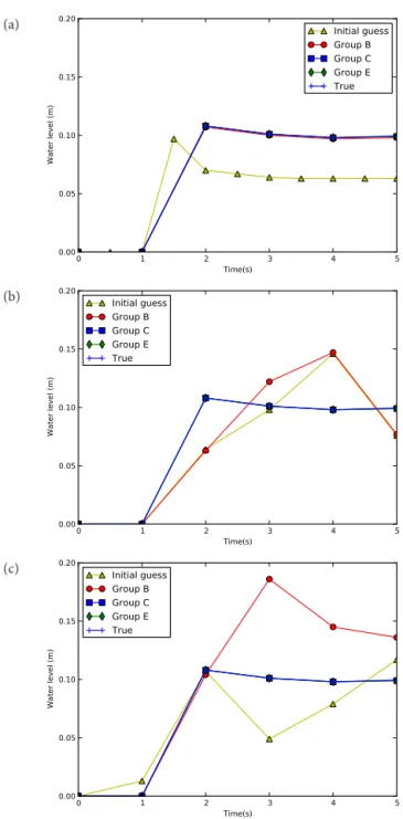
(a)
(b)
(c)
Figure 5.Water stage validation at the gauge point in(a)experiment series A,(b)experiment series B, and(c)experiment series C.
to become much closer to the true values. For example, the RMSEh decreased by 90 % when assimilating the
sin-gle flood extent att=24 s, and by about 93 % when further
assimilating flood extent at t=36 or 45 s (Table 4). These
results indicate that detailed content in the flood extent is important for the assimilation performance. Assimilation ex-periments also show that the proposed method can directly handle complex flood extents; e.g., the isolated islands in-side the flooded areas, with grid-based flood extents defined to be compatible with the numerical grids.
5 Assimilation of an actual remotely sensed flood extent Based on the findings of the previous numerical experiments, this section intends to investigate further the potential of the proposed data assimilation method using actual satellite re-mote sensing data (here, MODIS). The study area, Mengwa flood detention area (MFDA), is located at Fuyang, Anhui Province of China, on the middle reach of the Huaihe River. It is the most important region for flood control within this river basin. MFDA covers a narrow and elongated area of 180 km2 (Fig. 8a), with a population of 148 000 farming 120 km2of cropland. The domain is discretized using an un-structured grid (Fig. 8b) consisting of 1222 nodes and 1136 quadrilateral and triangular cells. The size of the cell edges ranges from 200 to 400 m. The bed elevation at each cell is extracted from a DEM of a 100 m resolution, which is gener-ated from a 1 : 2500 topographic map.
The data assimilation experiments are carried out based on the flood routing process over MFDA induced by the flood diversion event that happened in the summer of 2007. From 29 June to 15 July 2007, persistent heavy rain was ex-perienced in the Huaihe River basin. To reduce the risk of severe flooding that might cause significant economic and human loss downstream, MFDA was operated by opening the Wangjiaba gate (Fig. 8a) to receive flood water from the Huaihe River starting from 04:28 UTC, 10 July, with an order from the Chinese central government. Until 12 July 2007, the total diverted volume reached about 0.25×10⁹m3, which
effectively stored and retained flood water and hence re-duced flood risk. Figure 8 plots the 45 h inflow hydro-graph to MFDA through the flood gate, from 04:28 UTC, 10 July 2007.
Two MODIS instruments on the Terra and Aqua space-craft platforms have provided daily measurements with the global coverage since 1999. The 250 m resolution with daily revisits makes them particularly suitable for monitoring the changes of flooding over a floodplain. Herein, we down-loaded one scene of Aqua/MODIS Level 1B and geolocation data covering the whole MFDA from the Level 1 and At-mosphere Archive and Distribution System (LAADS). The MODIS data were acquired at 06:00 UTC with a 250 m reso-lution capturing the flood routing during the flood diversion event. Although MFDA was partly covered by light cloud at that moment, the image is of sufficient quality to identify the flood extent.
A simple method is adopted to extract the flood extent based on the luminance of the composite image from the band 7–2–1 combination. The luminanceLof each pixel is
firstly calculated using the following formula (Gonzales and Woods, 2002):
L=0.299b7+0.587b2+0.114b1, (11)
X
Y
0 20 40 60 80
0 5 10
15 Elev.: 0 0.05 0.1 0.15 0.2 0.25 0.3 0.35 0.4
X
0 20 40
h 0.4 0.3
0.2 0.1
X
0 20 40
h 0.4
0.3 0.2
0.1
X
0 20 40
h 0.4 0.3
0.2 0.1 (a)
(b)t= 24 s
(d) = 45 st
(c) t= 36 s
Cells where 0.001 m <h<0.01 m
water boundary lines at =0.0001 mh
Figure 6.Test case of a flood routing over three mounds.(a)Bed elevation and computational grids;(b)flood extent and water depth contour att=24 s;(c)flood extent and water depth contour att=36 s;(d)flood extent and water depth contour att=45 s.
0 0.01 0.02 0.03 0.04 0.05
0 10 20 30 40
time (s)
Guess H1-45 H1-36 H1-24 H2-45 H2-36 H2-24 H3-45 H3-36 H3-24 U-45 U-36 U-24 B-45 B-36 B-24
RMSE
(m)
h
time (s)
0 0.01 0.02 0.03 0.04 0.05
0 10 20 30 40
Guess B2-45 B2-36 B2-24 B2-36&45 B2-24&45 B2-24&36
RMSE
(m)
h
(a) (b)
Figure 7.The time series of RMS errors of water depth (RMSEh)in assimilation experiments with(a)lumped Manning’sn, and(b)
dis-tributed Manning’sn.
cover. The flood extent is then easily extracted over MFDA by setting a critical value of luminance as a threshold to sep-arate the water area from the image. However, due to the fact that the extraction of flood extent may be affected by the land surface, such as trees and vegetation cover (Smith, 1997), and that the current image is of a relatively low resolution of 250 m, there exist certain uncertainties in the boundary water line. In light of this, the concept of membership degree from the fuzzy set theory (Huang, 2000; Nguyen and Walker, 2006) is introduced as an indicator to determine the flood ex-tent. The degree of membership w quantifies the grade of
membership of an element to a fuzzy set, which is herein the possibility of a pixel being wet. A membership function may be written as (Huang, 2000)
w=
1
0.5+0.5 sin(b−πa·(Li−a+2b)) 0
, Li≤a
, a < Li≤b
, Li≥b
, (12)
whereLi is the luminance of pixelI, anda andbare the
upper and lower bounds of the luminance to separate the wa-ter and land. The degree of membershipw=0 andw=1
mean that pixeliis completely dry and wet, respectively. A
value between 0 and 1 characterize fuzzy members that are only partially wet/dry. Misclassification may also occur with this method. For those areas covered by heavy clouds, null values are given to the corresponding pixels and these cells are excluded from the evaluation of cost function.
From visual interpretation, we can identify that those ar-eas with luminanceLi less than 110 are covered by water
and hencea=110. The upper boundb is more difficult to
determine owing to the effects of complicated land cover. In this paper,b=121 and 126 are respectively examined. The
flood extents retrieved from fixed thresholds 110, 121, and 126 are shown in Figs. 9b–d.
115°50'0"E 115°50'0"E
115°40'0"E 115°40'0"E
115°30'0"E 115°30'0"E
3
2
°3
5'
0"
N
32
°3
5'
0
"N
32
°30
'0
"N
32
°3
0
'0
"N
32
°25'
0
"N
Huan ghe R
iver
Yang tzeRi
ver Ea
st
C
h
in
a
O
c
e
a
n
Huaihe River Gran
d Canna
l
±
9 4.5 0km Mengwa Flood Detention Area
Wangjiaba Gate
Caotaizhi Gate
Huaihe
River
0 400 800 1200 1600 2000
0.0 10.0 20.0 30.0 40.0 50.0 Time of flood diversion / h
Discharge(m
/s)
3
(b) (c)
(a)
Figure 8. (a)Mengwa flood detention area (MFDA);(b) unstruc-tured grid;(c)inflow discharge hydrograph.
Figure 9. (a) Luminance of MODIS image with band 7–2–1; (b)flood extent extracted from the fixed digital number threshold 110;(c)flood extent extracted from the fixed digital number thresh-old 121; (d)flood extent extracted from the fixed digital number threshold 126.
cost functionJis obtained as
J =1
2
0.5(1− h−hc |h−hc|)−w
2
h2. (13)
Based on this cost function, data assimilation experiments are conducted with a computational time step of 12 s. The simulation time is set to 36 h, starting from the gate opening at 04:28 UTC on 10 July 2007. The actual discharge hydro-graph for flood diversion to MFDA, as shown in Fig. 8c, is imposed through the inflow discharge boundary. Simulation starts from an originally dry floodplain. The critical water
(a)n0= 0.025 (b)n0= 0.8
First guess Assimilation
Mengwa, 2007-7-11 14:00
Figure 10.Comparing flood extents obtained before and after as-similation of the remotely sensed flood extent from MODIS image specified byb=126 (background map) when(a)n0=0.025; and
(b)n0=0.8. The solid line represents the boundary of the flood
ex-tent after assimilation, where water depth is equal tohc. The filled area is the flood extent computed by forward model withn0.
depth to derive the boundary line of flood extent from remote sensing data,hc, is set to 0.2 m.
The Manning roughness coefficient,n, was assumed to be
constant over the whole computational domain because of little knowledge about land use or cover. The control vari-able of the numerical experiments is the lumped Manning’s
n, namely the control vector contains only one element.
Giv-ing differentn0(Table 5), we carried out six numerical sim-ulations assimilating one single remotely sensed flood extent from MODIS data att=25.5 h withb=121 and 126. The
minimized cost functions of the experiments with b=126
are less than those withb=121, but the values are close to
their minimum for an independentb(Table 5).
Figure 10 shows the computed flood extents before and af-ter data assimilation. It can be observed that consistent flood extents are obtained in the assimilation experiments with dif-ferentn0by assimilating the flood-extent information from
MODIS data. Also, it is obvious that the computed flood ex-tents are improved after data assimilation has been performed in both experiments. The estimated flood extents are much closer to the one extracted from MODIS (Fig. 9). The find-ings are encouraging, which indicate that hydraulic informa-tion from satellite imagery can be directly assimilated into a 2-D dynamic flood model via the flood extent using the cost function, as suggested in this work.
We also identify a consistentnin the assimilation
exper-iments with differentn0, as listed in Table 5. The identified
nis about 0.2∼0.25, partly depending on n0. It is greater
than the empirical value of a normal floodplain, which may be caused by the loss of accuracy from the low-resolution MODIS data and uncertainties in the domain topography, etc. In addition, the minimization procedure of the 4D-Var method seems to be trapped in the local minimal value for differentn0in our experiments. Taking the experiments with
b=126 as an example, the optimized n is 0.208 if n0=
0.025 or 0.030, but it is close to 0.24 ifn0=0.5 or 0.8.
Table 5.The identifiednand the final cost functions in the application to MFDA.
Upper bound Final cost Decrease rate of Initial guess Identified of luminance,b function,J cost function (%) ofn,n0 n,n
126
28.118 81.2 0.025 0.208
28.127 78.0 0.030 0.208
28.432 14.6 0.500 0.249
28.319 24.2 0.800 0.240
121 49.071 70.6 0.030 0.219
48.937 18.6 0.800 0.240
25.0 27.0 29.0 31.0 33.0 35.0 37.0 39.0 41.0
0 0.1 0.2 0.3 0.4 0.5 0.6 0.7 0.8
Manning roughness coefficient,n
Cost
function,
J
Figure 11.The relationship between the cost function and the Man-ning’sn.
n(Fig. 11), two local minimal values of cost function exist
when nis close to 0.20 or 0.24. This leads to different
es-timations ofnin our experiments. The double minima may
originate primarily from the assumption of a constantnover
the study area with heterogeneous landscapes, which is in-consistent with the actual situation. Furthermore, insufficient data (a single low-resolution flood extent) may also lead to the appearance of double minima in the cost function.
6 Summary and conclusions
To the best of our knowledge, no attempt has been reported to directly assimilate the flood-extent data into a 2-D flood model in the framework of 4D-Var. In this work, a 4D-Var method incorporated with a new cost function is introduced to advance this research topic. The new approach has been validated using a series of numerical experiments undertaken for an idealized test case before applying to a realistic simula-tion in MFDA. The main results of this study are summarized as follows:
– A new cost function is defined to facilitate assimilation of flood-extent data directly using a 4D-Var method. While it can efficiently help the 2-D flood model to as-similate the spatially distributed flood dynamic informa-tion of the flood-extent data from remote sensing
im-agery, the current approach does not require those ad-ditional steps of retrieving water stage (Hostache et al., 2010). Since the flood extent is much easier to map from a remote sensing image than water stage and gradients (Schumann et al., 2009), the present scheme provides a more promising way of data assimilation for flood in-undation modeling. However, as a new data assimila-tion method for flood modeling, an interesting research question to answer is whether the direct assimilation of flood-extent data can improve the assimilation accuracy compared with the assimilation of water level observa-tions retrieved from the same data sources of satellite imagery. This is worth a comprehensive comparative study in the future, which may then provide a useful guideline for the practical applications of remote sens-ing data assimilation.
– Flood extent is a type of spatially distributed data and implicitly implies hydraulic information of flood rout-ing. The observed flood-extent data may provide an al-ternative to obtaining a denser time series, as stated by Roux and Dartus (2006), and to compensating for un-available field measurements during a flood event (Lai and Monnier, 2009). The assimilation of flood-extent data is suitable for improving flood modeling in the floodplains or similar areas (e.g., seasonal lakes with significant wetting and drying processes) with slowly varying bed slopes. However, it should be noted that this approach has its own limitation. If the flood extent does not contain enough hydraulic information, the assimila-tion exercise may fail. For example, in the case of flood inundation in a domain constrained by steep slopes, the water stage (but not the flood extent) varies evidently with time. Since the extent data do not actually repre-sent the physical evolution of such a flood event, they are not suitable for assimilation. Therefore, the corre-lation between extent and flood dynamics must be es-tablished before applying the current data assimilation scheme.
(250 m) is adopted in the application of MFDA. This implies that the proposed method may extend the usable data sources for assimilation to the imageries from most of satellites that are currently in orbit and that provide large spatial and temporal coverage.
Overall, this study shows that the assimilation of the flood-extent data is effective in improving flood modeling practice. Future work should be carried out to understand the full po-tential of this new way of making use of spatially distributed data from various existing satellites in data assimilation.
Acknowledgements. The research was supported by the
Na-tional Key Basic Research Program of China (973 Program) (2012CB417000) and the National Natural Science Foundation of China (grant no. 50709034 and no. 41071021). The authors also thank Guy Schumann, Renaud Hostache, and anonymous reviewer for their valuable comments for improving the paper’s quality.
Edited by: F. Pappenberger
References
Alsdorf, D. E., Rodríguez, E., and Lettenmaier, D. P.: Measur-ing surface water from space, Rev. Geophys., 45, RG2002, doi:10.1029/2006RG000197, 2007.
Andreadis, K. M., Clark, E. A., Lettenmaier, D. P., and Als-dorf, D. E.: Prospects for river discharge and depth esti-mation through assimilation of swath-altimetry into a raster-based hydrodynamics model, Geophys. Res. Lett., 34, L10403, doi:10.1029/2007GL029721, 2007.
Aronica, G., Bates, P. D., and Horritt, M. S.: Assessing the uncer-tainty in distributed model predictions using observed binary pat-tern information within GLUE, Hydrol. Process., 16, 2001–2016, doi:10.1002/hyp.398, 2002.
Atanov, G. A., Evseeva, E. G., and Meselhe, E. A.: Estimation of roughness profile in trapezoidal open channels, J. Hydraul. Eng., 125, 309–312, 1999.
Bateni, S. M., Entekhabi, D., and Jeng, D.-S.: Variational assim-ilation of land surface temperature and the estimation of sur-face energy balance components, J. Hydrol., 481, 143–156, doi:10.1016/j.jhydrol.2012.12.039, 2013.
Bélanger, E. and Vincent, A.: Data assimilation (4D-VAR) to fore-cast flood in shallow-waters with sediment erosion, J. Hydrol., 300, 114–125, doi:10.1016/j.jhydrol.2004.06.009, 2005. Begnudelli, L. and Sanders, B. F.: Conservative Wetting and
Dry-ing Methodology for Quadrilateral Grid Finite-Volume Mod-els, J. Hydraul. Eng., 133, 312–322, doi:10.1061/(ASCE)0733-9429(2007)133:3(312), 2007.
Brakenridge, G. R., Tracy, B. T., and Knox, J. C.: Orbital SAR remote sensing of a river flood wave, Int. J. Remote Sens., 19, 1439–1445, 1998.
Cacuci, D. G.: Sensitivity & Uncertainty Analysis, Vol. 1: Theory, 1st Edn., Chapman and Hall/CRC., 2003.
Crétaux, J.-F. and Birkett, C.: Lake studies from satellite radar altimetry, Comptes Rendus Geoscience, 338, 1098–1112, doi:10.1016/j.crte.2006.08.002, 2006.
Le Dimet, F.-X., Castaings, W., Ngnepieba, P., and Vieux, B.: Data assimilation in hydrology: variational approach, in: Data Assim-ilation for Atmospheric, Oceanic and Hydrologic Applications, 367–405, Springer, 2009.
Le Dimet, F.-X. and Talagrand, O.: Variational algorithms for analysis and assimilation of meteorological observations: the-oretical aspects, Tellus, 38A, 97–110, doi:10.1111/j.1600-0870.1986.tb00459.x, 1986.
Ding, Y.: Identification of Manning’s roughness coefficients in shallow water flows, J. Hydraul. Eng., 130, 501–510, doi:10.1061/(ASCE)0733-9429(2004)130:6(501), 2004. Durand, M., Andreadis, K. M., Alsdorf, D. E., Lettenmaier, D.
P., Moller, D., and Wilson, M.: Estimation of bathymetric depth and slope from data assimilation of swath altimetry into a hydrodynamic model, Geophys. Res. Lett., 35, L20401, doi:200810.1029/2008GL034150, 2008.
Fu, L. L. and Cazenave, A.: Satellite Altimetry and Earth Sciences. A handbook of Techniques and Applications, Academic Press, 2001.
Gilbert, J. C. and Lemaréchal, C.: Some numerical experiments with variable-storage quasi-Newton algorithms, Math. Program., 45, 407–435, 1989.
Giustarini, L., Matgen, P., Hostache, R., Montanari, M., Plaza, D., Pauwels, V. R. N., De Lannoy, G. J. M., De Keyser, R., Pfister, L., Hoffmann, L., and Savenije, H. H. G.: Assimilating SAR-derived water level data into a hydraulic model: a case study, Hydrol. Earth Syst. Sci., 15, 2349–2365, doi:10.5194/hess-15-2349-2011, 2011.
Gonzales, R. C. and Woods, R. E.: Digital Image Processing, 2nd Edn., Prentice Hall, 2002.
Hascoët, L. and Pascual, V.: TAPENADE 2.1 user’s guide, avail-able at: http://hal.archives-ouvertes.fr/inria-00069880/ (last ac-cess: 26 May 2013), 2004.
Honnorat, M., Marin, J., Monnier, J., and Lai, X.: Dassflow v1. 0: a variational data assimilation software for 2D river flows, avail-able at: http://hal.archives-ouvertes.fr/inria-00137447/ (last ac-cess: 26 May 2013), 2007.
Honnorat, M., Monnier, J., and Le Dimet, F.-X.: Lagrangian data assimilation for river hydraulics simulations, Comput. Vis. Sci., 12, 235–246, 2009.
Honnorat, M., Monnier, J., Rivière, N., Huot, É., and Le Dimet, F.-X.: Identification of equivalent topography in an open channel flow using Lagrangian data assimilation, Comput. Vis. Sci., 13, 111–119, 2010.
Hostache, R., Lai, X., Monnier, J., and Puech, C.: Assimilation of spatially distributed water levels into a shallow-water flood model. Part II: Use of a remote sensing image of Mosel River, J. Hydrol., 390, 257–268, doi:10.1016/j.jhydrol.2010.07.003, 2010.
Huang, J. Y.: Fuzzy Set and Its Application, Ningxia People’s Educ. Press Yinchuan China, 157–170, 2000.
Komma, J., Blöschl, G., and Reszler, C.: Soil moisture updating by Ensemble Kalman Filtering in real-time flood forecasting, J. Hydrol., 357, 228–242, doi:16/j.jhydrol.2008.05.020, 2008. Lai, X. and Monnier, J.: Assimilation of spatially distributed
Lee, H., Seo, D.-J., Liu, Y., Koren, V., McKee, P., and Corby, R.: Variational assimilation of streamflow into operational distributed hydrologic models: effect of spatiotemporal scale of adjustment, Hydrol. Earth Syst. Sci., 16, 2233–2251, doi:10.5194/hess-16-2233-2012, 2012.
Matgen, P., Hostache, R., Schumann, G., Pfister, L., Hoffmann, L., and Savenije, H. H. G.: Towards an automated SAR-based flood monitoring system: Lessons learned from two case studies, Phys. Chem. Earth Parts ABC, 36, 241–252, doi:10.1016/j.pce.2010.12.009, 2011.
Matgen, P., Montanari, M., Hostache, R., Pfister, L., Hoffmann, L., Plaza, D., Pauwels, V. R. N., De Lannoy, G. J. M., De Keyser, R., and Savenije, H. H. G.: Towards the sequential assimilation of SAR-derived water stages into hydraulic models using the Par-ticle Filter: proof of concept, Hydrol. Earth Syst. Sci., 14, 1773– 1785, doi:10.5194/hess-14-1773-2010, 2010.
Matgen, P., Schumann, G., Henry, J.-B., Hoffmann, L., and Pfis-ter, L.: Integration of SAR-derived river inundation areas, high-precision topographic data and a river flow model toward near real-time flood management, Int. J. Appl. Earth Obs. Geoinfor-mation, 9, 247–263, doi:10.1016/j.jag.2006.03.003, 2007. McLaughlin, D.: An integrated approach to hydrologic data
assim-ilation: interpolation, smoothing, and filtering, Adv. Water Re-sour., 25, 1275–1286, doi:16/S0309-1708(02)00055-6, 2002. Nguyen, H. T. and Walker, E. A.: A first course in fuzzy logic,
Chap-man & Hall/CRC, 2006.
Oberstadler, R., Hönsch, H., and Huth, D.: Assessment of the mapping capabilities of ERS-1 SAR data for flood map-ping: a case study in Germany, Hydrol. Process., 11, 1415– 1425, doi:10.1002/(SICI)1099-1085(199708)11:10<1415::AID-HYP532>3.0.CO;2-2, 1997.
Pappenberger, F., Beven, K., Frodsham, K., Romanowicz, R., and Matgen, P.: Grasping the unavoidable subjectivity in calibration of flood inundation models: A vulnerability weighted approach, J. Hydrol., 333, 275–287, doi:10.1016/j.jhydrol.2006.08.017, 2007a.
Pappenberger, F., Frodsham, K., Beven, K., Romanowicz, R., and Matgen, P.: Fuzzy set approach to calibrating distributed flood inundation models using remote sensing observations, Hydrol. Earth Syst. Sci., 11, 739–752, doi:10.5194/hess-11-739-2007, 2007b.
Pender, G. and Néelz, S.: Use of computer models of flood inunda-tion to facilitate communicainunda-tion in flood risk management, En-viron. Hazards, 7, 106–114, doi:10.1016/j.envhaz.2007.07.006, 2007.
Raclot, D.: Remote sensing of water levels on floodplains: a spatial approach guided by hydraulic functioning, Int. J. Remote Sens., 27, 2553–2574, doi:10.1080/01431160600554397, 2006. Reichle, R. H.: Data assimilation methods in the
Earth sciences, Adv. Water Resour., 31, 1411–1418, doi:10.1016/j.advwatres.2008.01.001, 2008.
Roux, H. and Dartus, D.: Use of parameter optimization to estimate a flood wave: Potential applications to remote sensing of rivers, J. Hydrol., 328, 258–266, doi:10.1016/j.jhydrol.2005.12.025, 2006.
Santos da Silva, J., Calmant, S., Seyler, F., Rotunno Filho, O. C., Cochonneau, G., and Mansur, W. J.: Water levels in the Amazon basin derived from the ERS 2 and ENVISAT radar altimetry missions, Remote Sens. Environ., 114, 2160–2181, doi:10.1016/j.rse.2010.04.020, 2010.
Schumann, G., Bates, P. D., Horritt, M. S., Matgen, P., and Pap-penberger, F.: Progress in integration of remote sensing–derived flood extent and stage data and hydraulic models, Rev. Geophys., 47, RG4001, doi:200910.1029/2008RG000274, 2009.
Schumann, G. J.-P., Neal, J. C., Mason, D. C., and Bates, P. D.: The accuracy of sequential aerial photography and SAR data for observing urban flood dynamics, a case study of the UK summer 2007 floods, Remote Sens. Environ., 115, 2536–2546, doi:10.1016/j.rse.2011.04.039, 2011.
Schumann, G., Matgen, P., Hoffmann, L., Hostache, R., Pappen-berger, F., and Pfister, L.: Deriving distributed roughness values from satellite radar data for flood inundation modelling, J. Hy-drol., 344, 96–111, doi:10.1016/j.jhydrol.2007.06.024, 2007. Schumann, G., Matgen, P., and Pappenberger, F.: Conditioning
wa-ter stages from satellite imagery on uncertain data points, Geosci. Remote Sens. Lett. IEEE, 5, 810–813, 2008.
Smith, L. C.: Satellite remote sensing of river inundation area, stage, and discharge: A review, Hydrol. Process., 11, 1427–1439, 1997. Talagrand, O. and Courtier, P.: Variational assimilation of meteoro-logical observations with the adjoint vorticity equation. I: The-ory, Q. J. Roy. Meteorol. Soc., 113, 1311–1328, 1987.
Toro, E. F.: Shock-Capturing Methods for Free-Surface Shallow Flows, 1st Edn., Wiley, 2001.