ISSN 0101-8205 www.scielo.br/cam
Infiltration condition and mouldability diagram
in resin injection moulding
LUCA MESIN
Department of Mathematics, Politecnico of Torino Corso Duca degli Abruzzi 24, Torino, 10129, Italy
E-mail: [email protected]
Abstract. This paper deals with the modelling of injection moulding processes taking into
account the deformability of the preform and the polymerisation of the resin. The coupled
flow–deformation problem in the infiltrated and dry region is formulated with the
correspond-ing boundary conditions and with the proper evolution equations determincorrespond-ing the motion of the
boundaries. An approximated analytical discussion is performed to obtain some estimates on the
infiltration velocity, helping in identifying a window of applicability in the parameters space (i.e.,
the mouldability diagram), which fits well with the numerical simulations.
Mathematical subject classification: 35K10, 35R35, 35L10.
Key words: injection moulding, deformable porous media, mouldability diagram.
1 Introduction
The high fluid pressure required in resin transfer moulding, Rudd et al. [32], and the high compliance of the porous preform can determine a significant de-formation of the preform during infiltration, Danis et al. [13], Kim et al. [19], Michand et al. Michaud et al. [27], Yamauchi and Nishida [37]. Such a defor-mation has great influence in the rate of the flow of the infiltrating resin and in the microstructure of the final product, Sommer and Mortensen [35]. Indeed the permeability of the preform depends strongly on the pore volume fraction and reduces more and more as the preform is compressed. The effects of deformation
are also important in the case of sandwich structure, with the displacement and deformation of foam cores during infiltration, Al-Hamdan et al. [5]. A recent review paper which considers the problem of deformation is Lacoste et al. [21]. In order to identify in advance possible inhomogeneities and damages in the reinforcing network, it is important to consider a detailed mathematical model which takes into account the deformation of the solid constituent. One possible framework to address the modelling of the infiltration of a fluid in a deformable porous medium is to adopt the mixture theory or, more precisely, the porous media theory. The first examples of this type of applications is in Preziosi et al. [30] and Preziosi [28].
In this paper, I assume that the preform is saturated (the case of a solid-liquid-air mixture is dealt with in Antonelli and Farina [2]). On the other hand, we take the effect of curing into account since it strongly affects the process increasing the viscosity of the resin, preventing the whole infiltration if the process pa-rameters are not chosen properly. These effects combined with the deformation of the solid preform have been studied in Farina and Preziosi [14], Farina and Preziosi [15]. The inertial effects can be neglected, since they are important only in processes induced by the sudden imposition of the injection pressure during the initial compression, giving rise to quickly decaying small oscillations of the wet border of the preform, as studied in Ambrosi [1], Ambrosi and Preziosi [3], Ambrosi and Preziosi [4], Mesin and Ambrosi [25].
min-imum pressure that provides the full infiltration at a certain process temperature, can be obtained by a deep study of the infiltration problem, which requires the mathematical modelling and the quantitative analysis of the process.
The aim of this work is then to study a mathematical model of the injection moulding process, and to perform an analytical and numerical discussion in order to help in improving the manufacturing procedure identifying the optimum set of operating parameters. The paper shows how a mathematical model can help identifying the mouldability diagram.
The model used is non linear and presents coupled equations modelling the inflow of a reactive resin undergoing polymerisation into a deformable preform. The coupling between the curing equation and the porous media equations mod-elling the preform causes the mathematical analysis of the problem to be fairly involved. Some analytical results can be found in the literature, under the sim-plifying assumption of a rigid preform, Billi [6], Billi [7], Billi and Farina [8]. In this paper some analytical results on the infiltration rate are obtained in the one-dimensional isothermal case, but considering both the deformation of the preform and the polymerisation of the resin. An upper bound for the infiltration velocity (and hence also a lower bound for the infiltration time) is given. A fur-ther analytical estimate for the infiltration velocity is also given, which fits well with the numerical simulations and allows to find out very simply the optimal values for the process parameters. The numerical analysis regards the full non-isothermal model and puts in evidence the quality of the non-isothermal estimates (see also Liu [24], for other results in the isothermal approximation).
After this introduction, the paper is organised as follows:
– the second section is devoted to a short introduction of the classical frame-work in which the model is developed;
– the third section illustrates the model in the one dimensional case and presents the mathematical problem;
– in the fourth section, the numerical analysis is explained and the numerical results are shown;
expressions for the motion of the infiltration front and some estimates on the mouldability diagram are given.
2 Mathematical model
A proper theoretical framework to model the injection moulding process is the theory of deformable porous media, which can be obtained on the basis either of mixture theory or of others averaging methods.
The physical assumptions of the mathematical model considered are the fol-lowing:
A1. inertia is negligible if compared to the stresses;
A2. theprinciple of constituent separationis assumed, which means that the Helmholtz free energy densities depend only on quantities related to their own constituent variable;
A3. surface tension and capillary effects are neglected; A4. small departures from thermal equilibrium are studied;
A5. the motion of the fluid through the skeleton is slow, in order to neglect the viscous effects compared to the pressure gradient;
A6. all the constituents have the same temperature.
Based on the previous assumptions, the classical model for a porous medium can be recovered introducing conservation laws for the mass, the momentum and the energy.
In the model a fundamental role is played by the fact that the resin undergoes a polymerisation processusually referred to ascuring cycle. The polymerisation process consists in an exothermic cross-linking chemical reaction which links monomers to build longer and longer polymers. The state of the reaction is described by the so-called degree of cure(orresin conversion)δc(x,t)defined as the ratio of the amount of heat H released by the curing reaction over the total heat of reaction Hc: δc(x,t)= H(Hx,t)
c [0, 1]. As the liquid is moving, the
evolution of the degree of cure can be modelled by
∂ δc
∂t +vf ·gradδc= fc(δc, ) , (2.1)
The curing reaction enters the model of the infiltration process by the two following effects:
– a supply termR =φfHcfc(δc, ), whereφf is the resin volume fraction, is introduced in the energy balance, due to the heat released by the reaction;
– a viscosity increase, which becomes dramatic (it blows up) as the resin approaches a stage known asgelation, indicted byδg.
Referring to Preziosi and Farina [29], in the Eulerian framework, the mathe-matical model for the wet (or infiltrated) region writes
∂φs
∂t +div(φsvs)=0,
divvc=div(φsvs+φfvf)=0,
φf(vf −vs)= − K
µ grad P,
divT′w−grad P =0,
ρC
∂
∂t +vs·grad
=ρf Cf K
µφf
grad P·grad
+div(k grad )+ 1
µgrad P·Kgrad P
+tr(T′
wgrad vs)+φf Hc fc,
∂ δc
∂t +vf ·grad δc = fc,
(2.2)
where the index f refers to the fluid component (a resin) and s to the solid preform,φdenotes the volume fractions (φf =1−φs, which corresponds to the saturation assumption),Kthe permeability tensor of the preform,T′
wthe excess stress tensor in the wet region, Pthe pore pressure,ρthe density of the mixture as a whole,C(Cf) the total (fluid) heat capacity,kthe heat conductivity tensor.
For the dry region, neglecting air, the following model is considered
∂φs
∂t +div(φsvs)=0, div T′
d =0,
ρsCs
∂
∂t +vs·grad
=div(ks grad )+tr(T′dgrad vs) ,
whereCs is the solid heat capacity,ks is the solid heat conductivity, T′d is the excess stress tensor in the dry region.
The previous model must be closed by specialising the constitutive relations for the viscosityµand the permeability tensorK, the stress tensors in both the wet and the dry region, and the particular form of the curing function fc.
3 One dimensional problem
We’ll consider the infiltration process to be pressure driven, with a constant pres-sure jumpPapplied over the wet region. A one dimensional approximation is studied. Such a model can approximate an infiltration process concerning gen-erally flat mould cavities, when edge effects are negligible; the flow simulation for arbitrary component geometries requires to take into account two or three dimensional models Rudd et al. [32]. The one dimensional model, even if feasi-ble to more restricted applications, allows to obtain some interesting analytical estimates.
Referring to Figure 1, the preform is considered to be fixed with a net on the right and the fluid to enter from the left solid border of the preform.
Figure 1 – Representation of the infiltration problem. The infiltrated (wet) region is
delimited by the two moving boundaries of the problem. The right border of the preform,
instead, is fixed by a web, which allows only the liquid to go through.
The resin is supposed to infiltrate a matrix initially compressed, presenting a constant volume fraction corresponding to the applied pressure (referring to Ambrosi and Preziosi [4], Mesin and Ambrosi [25], considering inertial terms and starting from a relaxed matrix, rapidly decaying oscillations affect the system only at the early times). The length of the compressed preform is denoted by L = φr
φcl, whereφr andφcare the volume fraction in the relaxed and compressed
the left solid border moves as a consequence of the relaxation of the matrix in the infiltrated region. Referring to Gurtin [16] and Wilmanski [36], the Lagrangian framework is introduced on the solid constituent, in order to fix the left solid border. Its position is indicated with X =0.
In the Lagrangian formulation it is convenient to introduce the so-calledvoid ratio e(X,t)as dependent variable, in place of the volume fraction:
e:= 1−φs
φs
. (3.1)
Furthermore, the following constitutive assumptions are considered:
– the stress tensor of the preform is elastic; the elasticity assumption is made in order to get a simpler model, for which some analytical estimates can be obtained (for a mathematical discussion of the viscoelastic case, see Ambrosi and Preziosi [4]); this assumption requires to neglect relaxation phenomena during the process considered (lasting less than 10s, see Fig-ure 3); for metal preforms, due to their elastic-plastic behavior, such an assumption is more critical; preforms constituted by glass fibres can be better approximated by an elastic model; in the one dimensional case, the elastic assumption means that the stress tensor is a function (which is supposed to be one to one) of the void ratio only;
– the permeability depends only on the void ratio (this is another approxi-mation, as permeability is in general also a function of the temperature).
The one dimensional mathematical model in Lagrangian coordinates in the wet regionis the following
∂e
∂t =
∂
∂X
G(e) µ(δc, )
∂e
∂X
ρC∂
∂t =ρfCf
K(1+e) µe
(1+er)2 (1+e)2
∂Tw′
∂X
∂ ∂X +1+er
1+e
∂ ∂X
k 1+er 1+e
∂ ∂X
+ 1
µ
(1+er)2
(1+e)2 K
∂Tw′
∂X
2
+Tw′ 1+er
1+e
∂ ∂X
K
µ ∂Tw′
∂X
+ e
1+eHcfc(δc, )
∂ δc
∂t =
1 e
G(e) µ(δc, )
∂δc
∂X + fc(δc, )
where Tw′ = Tw′(e)is the excess stress tensor in the wet region (note that it is positive in compression contrary to the customary convention) and the following function is introduced
G(e)= −(1+er)
2
(1+e)
d Tw′(e)
de K(e) , (3.3)
whereer is the void ratio corresponding to the relaxed preform. We note that equation (3.2.I) is parabolic, since the functionµ(δG(e)
c, )is positive.
However, its value approaches zero whenδc→δg(near gelation). Furthermore it is assumed that the derivative ofG(e)is a negative function of the void ratio, as it is usually the case in applications.
From equation (2.3.II), written in the one dimensional case, we have that the void ratio is constant in thedry regionin space and time. Hence, the model for the dry region reduces to the energy balance
ρsCs
∂
∂t =
(1+er)2 (1+ed
c)2
∂ ∂X
k ∂
∂X
. (3.4)
Let’s obtain now the constant value of the void ratio in the dry region. As the excess stress is constant across the infiltration front, we have
Td′(edc)=Tw′(ewc) , (3.5) where T′
d is the excess stress in the dry region andedc, ecw are the value of the void ratio at the dry and wet side of the infiltration front, respectively. Being the excess stress a one to one function of the void ratio, we can obtained
c once we know ew
c. Integrating in space equation (2.2.IV), in its one dimensional form, from zero to Xi, we have
Tw′(e(t, X =Xi))−Tw′(e(t, X =0))= −P. (3.6) The preform is stress free at the left border of the preform, so that
In the one dimensional case an evolution equation for the infiltration frontXi(t)
can be given: its velocity is a Lagrangian velocity, Wilmanski [36]; referring to Ambrosi [1] it can be written as
˙
Xi(t)= − 1
ew c
G(ewc)
µ(δc, )
∂e ∂X
X−i
. (3.8)
Referring to Liu [23], Muller [26], Preziosi and Farina [29], the following boundary conditions are considered
e(t, X =0)=er, w(t, 0)=i n(t) ,
δc(t, 0)=δi n(t) , ew(t, Xi)=ecw,
w(t, Xi(t))=d(t, Xi(t)) ,
ks +ecwkf 1+ew
c
∂w
∂X Xi(t) = ks 1+ed
c
∂d
∂X Xi(t) ,
d(t, L)=out(t) .
(3.9)
The initial conditions are
d(0, X)=o(X) ,
Xi(0)=0. (3.10)
In what follows, the following conditions are considered
– i n(t)=out(t)=o(X)=0, a constant; – δi n(t)=0, the curing develops inside the preform.
4 Numerical simulations
The free boundary problem introduced in the previous section is integrated using a front tracking method, Crank [11]. The space interval was uniformly sampled (100 samples). The front tracking method has the advantage of setting smaller time steps (defined as the time needed for the infiltration front to move to the next spatial sample point) when the infiltration velocity is higher and larger time steps when infiltration is slowing down, e.g. near gelation. When gelation occurs, the infiltration process and the numerical simulation stop.
Due to the variable time step, an unconditionally stable method has to be used, Bellomo and Preziosi [9]. An implicit finite difference method (a backward Euler method) for each equation was used.
Concerning the degree of cure equation, an implicit upwind method is used for the central nodes. The infiltration front, instead, is a characteristic of the hyper-bolic equation and then the degree of cure there is obtained by direct integration along such a characteristic.
Domain decomposition techniques, Bellomo and Preziosi [9], are used to in-terface the problems for the temperature in the two regions.
The numerical analysis refers to the infiltration of a thermosetting resin in a network of glass fibers. Referring to Kamal and Sourour [20], Lin et al. [22], Sourour and Kamal [34], I use the following specific expression for the isothermal cure rate of a thermosetting resin (a general purpose unsaturated polyester, see Kamal and Sourour [20] for details)
fc(δc, ):=
c1exp
− E1 R
+c2exp
− E2 R
δmc
c (1−δc)nc , (4.1)
and for the viscosity of the resin
µ (, δc)=
¯
µexp
Eµ
R
δg
δg−δc
cµ+dµδc
, if δc < δg,
∞ if δc≥δg,
(4.2)
Regarding the permeability, referring to Young et al. [38], the following rela-tion is used
K(φs)=K0eα(φ1−φs). (4.3) The stress-strain relation is extrapolated from the data reported in Kim et al. [19]
T′ =β(eγ φ−eγ φr) , (4.4)
whereβandγ are coefficients taking different values passing from the wet region to the dry one.
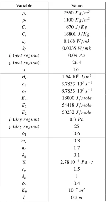
Table 1 summarizes all the parameters used in the simulations.
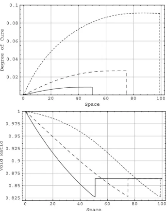
Figure 2 shows typical diagrams of the void ratio and the degree of cure. The discontinuity in the void ratio corresponds to the fact that different stress - void ratio relations are used in the wet and dry regions, according to the measurements in Kim et al. [19]. Continuity would be recovered if a viscoelastic model was used, Ambrosi and Preziosi [4].
However, in this paper I want to focus on the following features of the manu-facturing process:
– mouldability diagram;
– infiltration time;
– deformation of the preform.
The mouldability diagram presents the window of parameters for which the industrial process is successful. The key parameters under consideration are the injection pressurePand the process temperature0.
The infiltration time is the time taken by the infiltration process to be completed, in the case in which it is successful. After such a time the mould can be possibly heated to speed up the curing reaction.
Variable Value
ρs 2560K g/m3
ρl 1100K g/m3
Cs 670 J/K g
Cl 16801 J/K g
ks 0.168W/mk
kl 0.0335W/mk
β (wet r egi on) 0.09 Pa
γ (wet r egi on) 26.4
α 16
Hc 1.54 108 J/m3 c1 3.7833 105s−1 c2 6.7833 105s−1
Eµ 18000 J/mole
E2 54418 J/mole
E2 50232 J/mole
β (dr y r egi on) 0.3 Pa
γ (dr y r egi on) 25
φ1 0.6
mc 0.3
nc 1.7
δg 0.1
µ 2.78 10−4 Pa·s
cµ 1.5
dµ 1
φr 0.4
K0 10−9m2
l 0.3m
0 20 40 60 80 100 Space
0.02 0.04 0.06 0.08 0.1
Degree
of
Cure
0 20 40 60 80 100
Space 0.825
0.85 0.875 0.9 0.925 0.95 0.975 1
Void
Ratio
Figure 2 – Void ratio and degree of cure as a function of space (given in percent ofL).
The pressure is 1.2·105Paand the (constant) process temperature 350oK. In this case gelation occurs after the preform was infiltrated for the 99% of its length.
resin. Such a relaxation is studied integrating in time the velocity of the left solid border, that, referring to Billi and Farina [8], Preziosi and Farina [29], is given by
vl = K
µ ∂T′
w
∂φ ∂φ ∂x
x=xi
− K
µ ∂T′
w
∂φ ∂φ ∂x
x=xe
, (4.5)
where xi andxe are the Eulerian positions of the infiltration front and the left preform border, respectively. It needs to be mentioned that, because of the boundary conditions, deformation necessarily implies inhomogeneity in the final product.
correspondence with the injection pressure only.
In Figure 3 the mouldability diagram resulting from the simulations is shown. The left vertical axis reports the applied pressure, the horizontal one the constant environmental temperature in which the process takes place. The vertical axis on the right reports the deformation (which is in a one to one relation with the applied pressure). The five decreasing lines correspond to five different constant process times (time in which the infiltration is fulfilled), which can be named isochrones lines. The grey line is the limit below which gelation occurs: if we start from a point on such a line and increase the temperature and/or decrease the pressure then gelation occurs before the full infiltration is fulfilled. The grey line corresponds to processes for which the gelation time is equal to the infiltration time. It can be argued that from the operative viewpoint the best choice of injection pressure and temperature is that corresponding to a point just above the grey line, because it would minimize inhomogeneities in the final product. As suggested by Gonzales-Romero and Macosko [17] the diagram can be completed by adding the dash lines in Figure 3, corresponding to the lower limiting process temperature, the upper temperature limit above which degradation occurs, and the upper limit for the pressure, which accounts for the limited value for the injection unit and for mat tearing.
5 Estimates on the infiltration process
dura-Figure 3 – Mouldability diagram. The grey line represents the points for which the
infiltration time is equal to the gelation time, as a function of the temperature and the
pressure (corresponding to the percentage deformation shown on the right). Below this
line gelation occurs before completing the infiltration process. Along the full black
lines the infiltration time is the reported constant value. The dashed lines show the
lower temperature, the upper temperature limit (due to degradation) and the limit in the
pressure (due to the injection unit or to mat tearing). These latter dashed lines are not
studied in the paper.
tion the isothermal model is a good approximation. The isothermal assumption allows to simplify the model as follows
∂e ∂t s = ∂ ∂X G(e)
µ(δc)
∂e
∂X
X ∈ (0, Xi), t∈ (0,tf),
∂ δc
∂t
s = 1
e G(e)
µ(δc)
∂e
∂X
∂δc
∂X + fc(δc) X ∈ (0, Xi), t∈ (0,tf),
˙
Xi = −
1
ew c
G(ecw)
µ(δc)
∂e ∂X Xi
e(0,t)=er
e(Xi(t),t)=ewc
δc(X =0,t)=0,
Xi(t =0)=0,
(5.1)
from the arguments of the functionsµand fcto simplify the notation.
In what follows I first study the equation for the degree of cure, then the prop-erties of the degree of cure are used to obtain some estimates for the void ratio. The velocity of the infiltration front is then studied to estimate the infiltration time. Such a time is compared to the gelation time to know if the infiltration process is successful.
5.1 Some features of the equation for the degree of cure
The curing equation is hyperbolic with characteristics which go along the liquid. In particular the infiltration front is a characteristic. It is useful then to write this equation along the characteristics:
dδc
d t = fc(δc)
δc(t =τ )=0,
(5.2)
where the time derivative indicates total derivative along the characteristic,d td = ∂
∂t +Vf ∂
∂X, whereVf = − 1 e
G(e) µ(δc)
∂e
∂X is the Lagrangian velocity of the resin,τ is the instant in which the characteristic enters the infiltrated domain from the left preform border. The solution of the previous problem is
t−τ = δc
0 1
fc(δ)dδ=F(δc) . (5.3)
Being F(δc) an increasing function (as fc is a positive function), the previous equation is a one to one correspondence between timet and degree of cureδc with a parameterτ. If we fixτ and study (5.3) for increasing values of time, we readily notice that the degree of cure increases. On the other hand, fixing the timet, the degree of cure increases choosing smaller values of the parameterτ, which means considering a characteristic that entered the boundary X =0 at an earlier time. This means thatδcis also an increasing function of space and that the maximum always occurs at the infiltration front. We can then evaluate the gelation time as
tg=
δg
0 dδ
fc(δ), (5.4)
For the following, it is also important to study the derivative of the degree of cure w.r.t. X at the infiltration front. The ratio δc
X is studied at the early instant of time and then the limitt →0 is taken. We can evaluate the variation inδc studying equation (5.2) along the infiltration front
δc =
t
0
fc(δc(τ ))dτ ∼= fc(0)t. (5.5)
During the same time interval the advancement of the infiltration front can be obtained approximating (5.1.III):
X ∼=
2 ew
c G(ew
c)
µ(0) e
√
t, e=er −ewc , (5.6)
where the void ratio in the infiltration region is approximated by a straight line, which is justified by the fact that at early times the thickness of the wet region is very small. The result is coherent with the results obtained in Billi and Farina [8] for the case without curing.
We can now approximate the derivative of the degree of cure at early times as
∂δc
∂X ∼=
fc(0)√t
2ew
cG(ewc)µ(0)e
, (5.7)
which goes to zero astgoes to zero.
Now I study the evolution of the space derivative of the degree of cure at the infiltration front. Evaluating the derivative of (5.1.II) w.r.t. X, we can obtain the following equation for the space derivative of the degree of cure δX along the characteristics
dδX dt =
d fc dδc −
∂Vf
∂X
δX, (5.8)
where the total time derivative on the l.h.s. means derivation along a character-istic. The initial condition forδX must be non negative, since the degree of cure increases in space. Furthermore, the initial condition vanishes at the infiltration front, as shown by (5.7). Hence for the infiltration front
Regarding the space derivative of the degree of cure in all the wet region, we can obtain some qualitative information studying the ratio between the variation ofδcon two characteristics and the distance between such characteristics.
The variation ofδcdepends only on the difference between the times in which the characteristics enter the domain. Considering the choice of characteristic function fc(δc)introduced in Section 4, and evaluating numerically the integral in (5.3), we obtain that the increasing ofδcin time along a characteristic is well approximable with a straight line, for all the range of temperatures considered (from 300◦K to 400◦K).
The resin velocity is the velocity of the characteristics of the equation for the degree of cure. If curing is neglected, the infiltration velocity depends on time as a square root, Billi & Farina [8]. In such a case the resin covers one half of the length of the preform in one fourth of the infiltration time. Considering curing, the infiltration velocity reduces more and more in time: from the simulations reported in Figure 2, we can argue that the time taken by the resin to infiltrate the first half of the preform is of the order of 101 of the infiltration time. This means that initially the degree of cure is almost constant in a neighbour of the infiltration front with an extent of L2. As a consequence, also the viscosity is almost constant in that neighbour of the infiltration front, and, as the gradient of the resin velocity would be positive in the case of constant viscosity, we can argue that the dimensions of the neighbour of the infiltration front in which the degree of cure is almost constant are not reduced as the process proceeds.
5.2 Estimates on the void ratio near the infiltration front and on the infiltration process
The first step in our discussion of the evolution of the void ratio consists in fixing the moving boundary with the following Landau’s transformation
(X, t)−→
Y = X Xi(t), t
, (5.10)
so that X ∈ (0, Xi(t)] is mapped ontoY ∈ (0, 1] (see Figure 1). In order to avoid division by zero in the definition ofY in (5.10), we can consider the preform to be initially infiltrated in an arbitrary small region[0, b),b≪ L. The limitb →0 is finally discussed. Equation (5.1.I) becomes
∂e
∂t = Y
˙ Xi Xi
∂e
∂Y +
1 X2iµ(δc)
∂ ∂eG(e)
∂e
∂Y
2
+ G(e) Xi2
∂
∂δc
1
µ(δc)
∂δ
c
∂Y
∂e
∂Y +
G(e)
X2 iµ(δc)
∂2e
∂Y 2
,
(5.11)
wheree andδc are the void ratio and the degree of cure evaluated in the new variables(Y, t), respectively. An interesting qualitative result can be obtained from equation (5.11): the void ratio ranges between the boundary values and the extreme values are taken only at the boundary. Indeed it cannot have any maximum or minimum point in the interior of the domain by the maximum principle for parabolic equations (if a maximum point exists, its value has to decrease, and vice versa for the minimum; given the monotonous initial data, maxima and minima cannot exist). This means that the infiltration velocity is non negative in all the wet region and can only stop as an effect of the increasing of the viscosity, since the pressure gradient does not vanish at any point in the wet region.
give some suggestions of the mathematical reason why this happens studying the following problem for the differencewbetween the void ratio and the straight linevconnecting the boundary points
w(t, Y)=e(t, Y)−v(Y) where v(Y)=er −e Y, e=er −ec,
∂w
∂t =
G Xi2µ
∂2w
∂Y2 +
∂w
∂Y −e
G′
Xi2µ
∂w
∂Y −e
− Y X2i
1 ec
G
µ
∂w
∂Y −e Y=1−
Gµ′
Xi2µ2
∂δc
∂Y
w(t=0, Y)=0, w(t, Y =0)=0, w(t, Y =1)=0
(5.12)
where I supposed to approximate with a straight line the initial condition in the initially infiltrated region [0, b). The first term in the r.h.s. accounts for diffusion; the other three terms can be considered as sources. The first two sources are negative, whereas the last is non negative: this means that the void ratio is under the straight line till the positive source remains smaller than the negative ones. This condition is verified at the beginning of the infiltration process, since∂δc
∂Y ∼=0. This means that the void ratio is initially under the straight linev(Y)(for the maximum principle). The positive source is proportional to the derivative w.r.t. Y of the degree of cure so that it vanishes at the infiltration front. This means that there is always a neighbour of the infiltration front in which the source term is negative. Furthermore, at the end of Section 5.1 I argued that in a neighbour of the infiltration region with dimensions of the order of a half of the infiltrated preform the contribution due to this term is expected to be smaller than the other ones, and therefore in the same neighbour the total source term is negative.
the straight line between the boundary values near the left border only for large times.1
The positive source, if sufficiently large, can affect also the region near the infiltration front, due to diffusion. Nevertheless, the simulations suggest that this cannot happen, for all the parameters of interest.
In this way we can obtain a bound for the derivative ofe(t, X)w.r.t. X and, as a consequence, the following bound for the velocity of the infiltration front
˙
Xi < − 1 ew
c
G(ecw) µ(δc)
ec−er
Xi , (5.13)
where I used the fact that the space derivative ofe(X, t)at the infiltration front is less in modulus than the slope of the straight line between the boundary values. From the previous estimate we obtain the following bound for the evolution of the infiltration front
Xi(t) <
2e ew
c G(ew
c)
t
0 1
µ(δc(τ ))
dτ +b, (5.14)
whereδc(t)is recovered studying the equation for the degree of cure along the infiltration front. The term b in the expression (5.14) can be dropped, as it is arbitrarily small.
An important information can be obtained from the previous analysis: we can determine if the infiltration will be successful or not, controlling if the full infiltration is achieved. In fact computing (5.14) for t = tg, where tg is the gelation time given by (5.4), we can conclude that if
L =l1+ec 1+er >
2e ew c
G(ew c)
tg
0 1
µ(δc(τ ))
dτ (5.15)
then full infiltration cannot be achieved.
1It is worth noticing the dependence of the qualitative shape of the void ratio and the parameters.
Another useful relation can be obtained merging (5.2) and (5.14): in fact, one can deduce the following estimate
Xi(δc) <
2e ew
c G(ew
c)
δc
0
1
µ(δ)fc(δ)dδ , (5.16)
that is if
L >
2e ew
c G(ew
c)
δg
0
1
µ(δ)fc(δ)dδ (5.17)
the process is certainly incomplete.
In order to give a better approximation of the velocity of infiltration I study further the problem (5.1) in a neighbour of the infiltration front. For example, a second order approximation of the solutione(X,t)can be used near the infiltra-tion front, substituting the first and second derivative in equainfiltra-tion (5.11). In this case two parameters need to be determined, but only one equation is available. One way to proceed is to fix a constraint, choosing a particular kind of solution. In the following we examine as a set of trial solutions the family of parabolas connecting the conditions (5.1.IV) and (5.1.V), with a positive slope atY =1
h(Y)= −eY +er +αY(Y −1) , α∈ [0, e]. (5.18) Indeed, from the simulations we can note that the void ratio at a fixed time can be approximated well by a parabola, except when the resin is about to gel. I choose the parabola with convexity such that the r.h.s. of equation (5.11) evaluated at the infiltration front (i.e., in a point in which the void ratio is constant in time) vanishes. This occurs when
−β(ewc)(α−e)2+2αG(ewc)=0, (5.19) where
β(ewc)= − ∂ ∂eG(e)
ew c
+ G(e w c) ew
c
>0. (5.20)
The unique solution of (5.19) belonging to [0, e] (hence giving a positive infiltration velocity) is
α0=
β(ew
c)e+G(ewc)−
G(ew
c)2+2β(ecw)eG(ewc)
β(ew c)
The following estimates are obtained for the infiltration velocity
˙
Xi ∼= G(e w c) ew
cµ(δc(Xi, t))
e−α0
Xi ; (5.22)
and for the infiltration front
Xi(t) ∼=
2e−α0 ew
c
G(ew c)
t
0 1
µ(δc(τ ))
dτ . (5.23)
It is worth noticing that the value ofα0only depends on the value of the void ratio at the infiltration front. It does not depend on the degree of cure, because the derivative of the degree of cure w.r.t. Y vanishes at the infiltration front. Since the void ratio at the infiltration front is constant in time,α0is also constant in time.
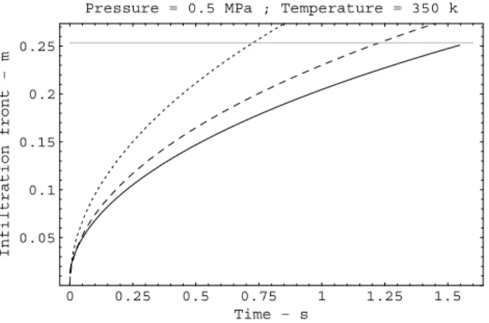
Figure 4 shows a comparison between the numerical results concerning the full model and the estimates (5.14) and (5.23), for two representative examples of process.
Substitutingewithe−α0in equation (5.16) we can obtain the following approximated expression to test if the full infiltration can be obtained
Xi(δc)∼=
2e−α0 ew
c
G(ew c)
δc
0
1
µ(δ)fc(δ)dδ . (5.24)
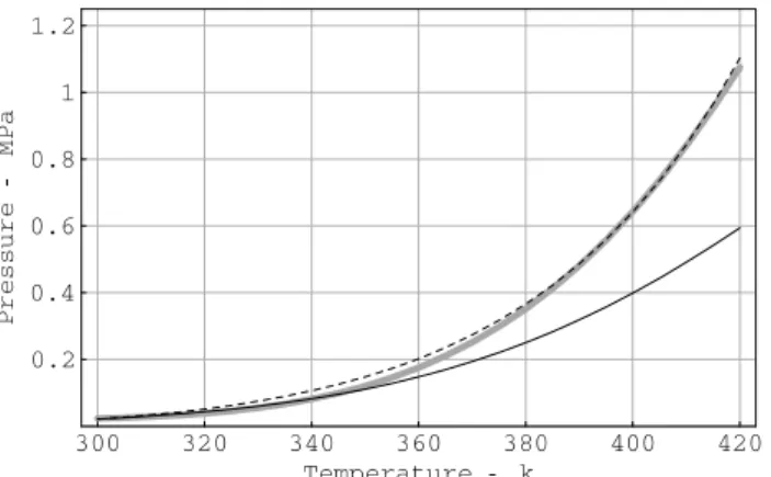
Figure 5 shows the limiting lines for which the gelation time is equal to the infiltration time: the full line refers to the approximation for the velocity of the front given by the correspondent equation of the inequality (5.16), the dashed line refers to equation (5.24), the grey line to the numerical analysis of the full model. Comparing the grey with the dash line, we can argue that estimate (5.24) gives a quite good approximation for the infiltration velocity. Comparing the grey with the full line we can say that the bound for the infiltration velocity (5.13) is close to the numerical results only for low pressure values.
Remark. As mentioned in the introduction, another way to drive the process is imposing the inflow velocityui nof the fluid instead of applying a pressure. If ui n is constant in time, referring to Ambrosi [1], the final time of infiltration is given by
Tf i n =
erL
0 0.25 0.5 0.75 1 1.25 1.5 Time s
0.05 0.1 0.15 0.2 0.25
Infiltration
front
m
Pressure 0.5 MPa ; Temperature 350 k
0 0.2 0.4 0.6 0.8 1 1.2 1.4
Time s 0.05
0.1 0.15 0.2 0.25 0.3
Infiltration
front
m
Pressure 0.5 MPa ; Temperature 400 k
Figure 4 – Lagrangian position of the infiltration front as a function of time: comparison
between the numerical solution (full line) and those obtained using the estimates (5.14)
(dot line) and (5.23) (dash line). Figure above a successful process is shown, figure
below an unsuccessful one (the length of the compressed preformLis indicated by the
horizontal grey line).
In the case of non constant inflow velocity, the final time can be obtained from the following implicit expression
Tf i n
0
ui n(τ )dτ = erL
1+er . (5.26)
Figure 5 – Results on the analytical estimates for the production process: the grey line
is obtained by numerical simulations; the dashed line refers to the approximation of the
void ratio with a parabola (see equation (5.23)); the full line refers to the approximation
of the void ratio with a straight line (see (5.13); under such a line gelation occurs for
sure).
have the following condition for the process to be successful
ui n> erL (1+er)δg
0 dδ fc(δ)
. (5.27)
6 Conclusions
A one dimensional mathematical model of the infiltration of an incompressible resin through a deformable solid porous medium (modelling a preform) has been considered, in the framework of mixture theory. The model has been applied to the industrial process of pressure driven resin injection moulding, considering an elastic preform.
Finally the numerical analysis gives the mouldability diagram, presenting the window of applicability in the parameter space.
It is worth noticing that in injection processes, the resin, the fibres and the mould are usually preheated at different temperatures. In such a case, assumption A6 (see Section 2) is not satisfied and an isothermal model would be a row approximation. It can be expected that obtaining analytical estimates for the case of non-isothermal models is a very difficult task, beyond the aims of this papers. Nevertheless, on the basis of the results of this paper, an approximate analysis of the isothermal model is suggested. Numerical analysis of non-isothermal models have been developed in the literature of non-non-isothermal liquid moulding processes (see for example Bruschke and Advani [10], Shojaei et al. [33]).
In conclusion, the main contribution of the paper is the mathematical analysis of a one dimensional mathematical model of the infiltration of an incompressible resin through a deformable solid porous medium introduced in previous works (see Ambrosi [1], Ambrosi and Preziosi [4]). Such an analysis provides some estimates of the infiltration process in the isothermal case. Further analytical analysis (supported by numerical simulations) is needed to extend the results of the paper to the three dimensional, non-isothermal case.
Acknowledgment. The author is grateful to Prof. Luigi Preziosi for his help in the preparation of the paper.
REFERENCES
[1] D. Ambrosi,Infiltration through deformable porous media. ZAMM,82(2002), 115–124.
[2] D. Antonelli and A. Farina,Resin transfer moulding: Mathematical modelling and numerical simulation. Composites A,30(1999), 1367–1385.
[3] D. Ambrosi and L. Preziosi,Modeling matrix injection through elastic porous preforms. Composites Part A, 29 (1998), 5–18.
[4] D. Ambrosi and L. Preziosi,Modeling injection molding processes with deformable porous preforms. SIAM J. Appl. Math.,61(2000), 22–42.
[6] L. Billi,Incompressible flows through porous media with temperature variable parameters. Nonlinear Anal.,31(1998), 363–383.
[7] L. Billi,Non-isothermal flows in porous media with curing. Eur. S. Appl. Math.,8(1997), 623–637.
[8] L. Billi and A. Farina,Unidirectional infiltration in deformable porous media: mathematical modeling and self-similar solution. Quart. Appl. Math.,58(2000), 85–101.
[9] N. Bellomo and L. Preziosi,Modelling Mathematical Methods and Scientific Computation. CRC Press, 1995.
[10] M.V. Bruschke and S.G. Advani,A Numerical Approach to Model Non-isothermal, Viscous flow with Free Surfaces through Fibrous Media. International Journal of Numerical Methods in Fluids,19(1994), 575–603.
[11] J. Crank,Free and Moving Boundary Problems. Clarendon Press, 1984.
[12] T.W. Clyne and J.F. Mason,The squeeze infiltration process for fabrication of metal matrix composites. Metall. Trans. A,18A(1987), 1519–1530.
[13] M. Danis, C. Del Borrello, E. Lacoste and O. Mantaux,Infiltration of fibrous preform by a liquid metal: Modelization of the preform deformation. Proceeding of the ICCM 12, Paris, 9 (1999).
[14] A. Farina and L. Preziosi,Non-isothermal injection moulding with resin cure and preform deformability. Composites A,31(2000), 1355–1372.
[15] A. Farina and L. Preziosi,Infiltration processes in composite materials manufacturing: Modeling and qualitative results, [inComplex Flows in Industrial Processes, Ed. Fasano A.–Kluwer], 281–306 (2000).
[16] M.E. Gurtin,An Introduction to Continuum Mechanics. Academic Press, (1981).
[17] V.M. Gonzales-Romero and C.W. Macosko,Process parameters estimation for structural reaction injection moulding and resin transfer moulding. Polymer Eng. Sci., 30(1990), 142–146.
[18] V.M. Gonzales-Romero and C.W. Macosko,Design strategies for composite reaction in-jection moulding and resin transfer moulding. Proc. ANTEC 86, 45t hAnnual Conference, Society of Plastics Engineers Inc., 1292–1295.
[19] Y.R. Kim, S.P. McCarthy and J.P. Fanucci,Compressibility and relaxation of fiber reinforce-ments during composite processing. Polymer Compos.,12(1991), 13–19.
[20] M.R. Kamal and S. Sourour, Kinetics and thermal characterization of thermoset cure. Polymer Eng. Sci.,13(1973), 59–64.
[22] R.J. Lin, L.J. Lee and M.J. Lion,Non–isothermal mold filling and curing simulation in thin cavities with preplaced fiber mats. Int. Polymer Process,6(1991), 356–369.
[23] I.S. Liu, On chemical potential and incompressible porous media. J. Mech.,19(1980), 327–342.
[24] X.L. Liu,Isothermal flow simulation of liquid composite molding. Composites Part A,31 (2000), 1295–1302.
[25] L. Mesin and D. Ambrosi,Inertial Effects in Composite Materials Manufacturing. J. Eng. Math.,50(2004), 379–398.
[26] I. Muller,Thermodynamics of mixtures of fluids. J. Mech.,14(1975), 267–303.
[27] V.J. Michaud, J.L. Sommer and A. Mortensen,Infiltration of a fibrous prefrom by a pure metal. Part V. Influence of preform compressibility. Metall. Mater. Trans. A,30(1999), 471–482.
[28] L. Preziosi,The theory of deformable porous media and its applications to composite material manufacturing. Surv. Math. Ind.,6(1996), 167–214.
[29] L. Preziosi and A. Farina,Deformable porous media and composites manufacturing, [in
Heterogeneous media, Ed. Markov K., Preziosi L.–Birkhauser] (2000).
[30] L. Preziosi, D.D. Joseph and G. Beavers,Infiltration of initially dry, deformable porous media. Int. J. Multiphase Flows,22(1996), 1205–1222.
[31] M.M. Reboredo and A.J. Rojas,Molding by reactive injection of reinforced plastics. Polymer Eng. Sci.,28(1988), 485–490.
[32] C.D. Rudd, A.C. Long, K.N. Kendall and C.G.E. Mangin,Liquid Moulding Technologies. Woodhead Publishing Limited, (1997).
[33] A. Shojaei, S.R. Ghaffarian and S.M.H. Karimian,Simulation of the three-dimensional non-isothermal mold filling process in resin transfer molding. Composites Science and Technology,63(2003), 1931–1948.
[34] S. Sourour and M.R. Kamal,Differential scanning calorimetry of epoxy cure: Isothermal cure kinetics. Thermodyn. Acta,14(1976), 41–59.
[35] J.L. Sommer and A. Mortensen,Forced unidirectional infiltration of deformable porous media. J. Fluid Mech.,311(1996), 193–215.
[36] K. Wilmanski, Thermo-Mechanics of Continua. Springer, (1998).
[37] T. Yamauchi and Y. Nishida,Infiltration kinetics of fibrous preforms by aluminum with solidification. Acta Metall. Mater.,21(1987), 172–188.