K. D. Jensen
Dantec Dynamics Inc.200 Williams Dr Ramsey, NJ 07446 USA [email protected]
Flow Measurements
This paper will review several techniques for flow measurements including some of the most recent developments in the field. Discussion of the methods will include basic theory and implementation to research instrumentation. The intent of this review is to provide enough detail to enable a novice user to make an informed decision in selecting the proper equipment to solve a particular flow measurement problem.
Keywords: Flow measurements, hot-wire anemometry, Laser-Doppler Anemometry (LDA), particle image velocimetry
Introduction
Almost all industrial, man-made flows are turbulent. Almost all naturally occurring flows on earth, in oceans, and atmosphere are turbulent. Therefore, the accurate measurement and calculation of turbulent flows has wide ranging application and significance.
i j ij i
f X Dt
Du U
w wW
U . (1)
In general, turbulent motion is 3-D, vortical, and diffusive making the governing Navier-Stokes equation (above) very hard (or impossible) to solve in most real applications, thus the need to measure flow.1
Early turbulence research has been complemented by experimental methods that included pressure measurements and by the point measurement technique of Hot Wire Anemometry (HWA). Particular difficulties in using these intrusive methods include, reversing flows, vortices, and highly turbulent flows. In addition, intrusive probes are subject to non-linearity (require calibration), sensitivity to multi-variable effects (temperature, humidity, etc.), and breakage among other problems.
With developments of lasers in the mid 1960’s non-intrusive flow measurement became practical. Soon after the introduction of gas lasers, Laser-Doppler Anemometry (LDA) was developed by Yeh and Cummins. This was one of the most significant advances for fluid diagnostics since we now had a nearly ideal transducer. Specifically, the output is exactly linear, no calibrations are required, the output has low noise, high frequency response and velocity is measured independently of other flow variables. During the last three decades, the LDA technique has witnessed significant advancements in terms of optical methods such as fibers, as well as, advanced signal processing techniques and software development. In addition, the LDA method has been extended to the Phase Doppler technique for the measurement of particle and bubble size along with velocity.
The rapid development within lasers and camera technology opened the possibility for qualifying (flow visualization) and later on quantifying whole flow field measurement. The development of Particle Image Velocemetry (PIV) has become one of the most popular instruments for flow measurements in numerous applications. Modern developments of camera and laser technology, as well as PIV software, continue to improve the performance of the PIV systems and their applicability to difficult flow measurements. In addition to the instantaneous measurement of the flow, a time resolved measurement is now possible with high frequency lasers and high frame rate cameras. Particle and bubble sizing is also possible with a modified PIV system that includes a second camera. Planar Laser Induced Fluorescence (PLIF) is now available as
Presented at ENCIT2004 – 10th Brazilian Congress of Thermal Sciences and Engineering, Nov. 29 -- Dec. 03, 2004, Rio de Janeiro, RJ, Brazil.
Technical Editor: Atila P. Silva Freire.
standard measurement systems for concentration and temperature. The PLIF systems are especially useful for heat transfer and mixing studies.
Point Versus Full Field Velocity Measurement
Techniques:
Advantages and Limitations
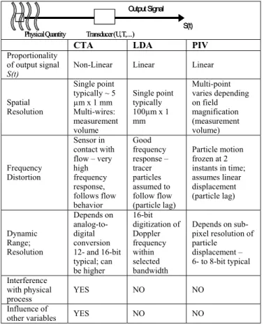
Hot Wire Anemometry (HWA), Laser Doppler Anemometry (LDA), and Particle Image Velocimetry (PIV) are currently the most commonly used and commercially available diagnostic techniques to measure fluid flow velocity. The great majority of the HWA systems in use employ the Constant Temperature Anemometry (CTA) implementation. A quick comparison of the key transducer properties of each technique is shown in Table 1 with expanded details on spatial resolution, temporal resolution and calibration provided in the following sections.
Table 1. Transducer comparison of commonly used velocity measurement diagnostics.
Output Signal S(t)
PhysicalQuantity Transducer U T( , ,...)
Output Signal S(t)
PhysicalQuantity Transducer U T( , ,...)
CTA LDA PIV
Proportionality of output signal
S(t)
Non-Linear Linear Linear
Spatial Resolution
Single point typically ~ 5 µm x 1 mm Multi-wires: measurement volume
Single point typically 100µm x 1 mm
Multi-point varies depending on field magnification (measurement volume)
Frequency Distortion
Sensor in contact with flow – very high frequency response, follows flow behavior
Good frequency response – tracer particles assumed to follow flow (particle lag)
Particle motion frozen at 2 instants in time; assumes linear displacement (particle lag)
Dynamic Range; Resolution
Depends on analog-to-digital conversion 12- and 16-bit typical; can be higher
16-bit digitization of Doppler frequency within selected bandwidth
Depends on sub-pixel resolution of particle
displacement – 6- to 8-bit typical
Interference with physical process
YES NO NO
Influence of
Spatial Resolution
High spatial resolution is a must for any advanced flow diagnostic tool. In particular, the spatial resolution of a sensor should be small compared to the flow scale, or eddy size, of interest. For turbulent flows, accurate measurement of turbulence requires that scales as small as 2 to 3 times the Kolmogorov scale be resolved. Typical CTA sensors are a few microns in diameter, and a few millimeters in length, providing sufficiently high spatial resolution for most applications. Their small size and fast response make them the diagnostic of choice for turbulence measurements.
The LDA measurement volume is defined as the fringe pattern formed at the crossing point of two focused laser beams. Typical dimensions are 100 microns for the diameter and 1 mm for the length. Smaller measurement volumes can be achieved by using beam expansion, larger beam separation on the front lens, and shorter focal length lenses. However, fewer fringes in the measurement volume increase the uncertainty of Doppler frequency estimation.
A PIV sensor is the subsection of the image, called an “interrogation region”. Typical dimensions are 32 by 32 pixels, which would correspond to a sensor having dimensions of 3 mm by 3 mm by the light sheet thickness (~1mm) when an area of 10 cm by 10 cm is imaged using a digital camera with a pixel format of 1000 by 1000. Spatial resolution on the order of a few micrometers has been reported by (Meinhart, C. D. et.al, 1999) who have developed a micron resolution PIV system using an oil immersion microscopic lens. What makes PIV most interesting is the ability of the technique to measure hundreds or thousands of flow vectors simultaneously.
Temporal Resolution
Due to the high gain amplifiers incorporated into the Wheatstone Bridge, CTA systems offer a very high frequency response, reaching into hundreds kHz range. This makes CTA an ideal instrument for the measurement of spectral content in most flows. A CTA sensor provides an analog signal, which is sampled using A/D converters at the appropriate rate obeying the Nyquist sampling criterion.
Commercial LDA signal processors can deal with data rates in the hundreds of kHz range, although in practice, due to measurement volume size, and seeding concentration requirements, validated data rates are typically in the ten kHz, or kHz range. This update rate of velocity information is sufficient to recover the frequency content of many flows.
The PIV sensor, however, is quite limited temporally, due to the framing rate of the cameras, and pulsing frequency of the light sources used. Most common cross-correlation video cameras in use today operate at 30 Hz. These are used with dual-cavity Nd:Yag lasers, with each laser cavity pulsing at 15 Hz. Hence, these systems sample the images at 30 Hz, and the velocity field at 15 Hz. High framing rate
CCD cameras are available that have framing rates in the ten kHz range, albeit with lesser pixel resolution. Copper vapor lasers offer pulsing rates up to 50 KHz range, with energy per pulse around a fraction of one mJ. Hence, in principle, a high framing rate PIV system with this camera and laser combination is possible. But, in practice, due to the low laser energy, and limited spatial resolution of the camera, such a system is suitable for a limited range of applications.
Recently, however, CMOS-based digital cameras have been commercialized with framing rates of 1 KHz and pixel resolution of 1k x 1k. Combined with Nd:Yag lasers capable of pulsing at several kHz with energies of 10 to 20 mJ/pulse, this latter system brings us one step closer to measuring complex, three-dimensional turbulent flow fields globally with high spatial and temporal resolution. The vast amount of data acquired using a high framing rate PIV system,
however, still limits its common use due to the computational resources needed in processing the image information in nearly real time, as is the case with current low framing rate commercial PIV systems.
Summary of Transducer Comparison
In summary, the point measurement techniques of CTA and LDA can offer good spatial and temporal response. This makes them ideal for measurements of both time-independent flow statistics, such as moments of velocity (mean, rms, etc) and time-dependent flow statistics such as flow spectra and correlation functions at a point. Although rakes of these sensors can be built, multi-point measurements are limited mainly due to cost.
The primary strength of the global PIV technique is its ability to measure flow velocity at many locations simultaneously, making it a unique diagnostic tool to measure three dimensional flow structures, and transient phenomenon. However, since the temporal sampling rate is typically 15 Hz with today’s commonly used 30 Hz cross-correlation cameras, the PIV technique is normally used to measure instantaneous velocity fields from which time independent statistical information can be derived. Cost and processing speed are currently the main limiting factors that influence the temporal sampling rate of PIV.
Intrusive and Non-Intrusive Measurement Techniques
Most emphasis in recent times has been in the development of non-intrusive flow measurement techniques, for measuring vector, as well as, scalar quantities in the flow. These techniques have been mostly optically-based, but when fluid opaqueness prohibits access, then other techniques are available. A quick overview of several of these non-intrusive measurement techniques is given in the next few sections for completeness. More extensive discussion on these techniques can be found in the references cited.
Particle Tracking Velocimetry (PTV) and Laser Speckle
Velocimetry (LSV)
Just like PIV, PTV and LSV measure instantaneous flow fields by recording images of suspended seeding particles in flows at successive instants in time. An important difference among the three techniques comes from the typical seeding densities that can be dealt with by each technique. PTV is appropriate with “low” seeding density experiments, PIV with “medium” seeding density and LSV with “high” seeding density. The issue of flow seeding is discussed later in the paper.
Historically, LSV and PIV techniques have evolved separately from the PTV technique. In LSV and PIV, fluid velocity information at an “interrogation region” is obtained from many tracer particles, and it is obtained as the most probable statistical value. The results are obtained and presented in a regularly spaced grid. In PIV, a typical interrogation region may contain images of 10-20 particles. In LSV, larger numbers of particles in the interrogation region scatter light, which interfere to form speckles. Correlation of either particle images or speckles can be done using identical techniques, and result in the local displacement of the fluid. Hence, LSV and PIV are essentially the same technique, used with different seeding density of particles. In the rest of the chapter, the acronym PIV will be used to refer to either technique.
Image Correlation Velocimetry (ICV)
Tokumaru and Dimotakis, (1995) introduced image correlation velocimetry (ICV) with the purpose of measuring imaged fluid motions without the requirement for discrete particles in the flow. Schlieren based image correlation velocimetry was recently implemented by Kegrise and Settles (2000) to measure the mean velocity field of an axisymetric turbulent free-convection jet. Also recently, Papadopoulos, (2000) demonstrated a shadow image velocimetry (SIV) technique, which combined shadowgraphy with PIV to determine the temperature field of a flickering diffusion flame. Image correlation was also used by Bivolaru et al. (1999) to improve on the quantitative evaluation of Mie and Rayleigh scattering signal obtained from a supersonic jet using a Fabry-Perot interferometer. Although such developments are novel, we are still far from being able to fully characterize a flow by complete simultaneous measurements of density, temperature, pressure, and flow velocity.
Doppler Ultrasonic Velocimetry
Doppler ultrasound technique was originally applied in the medical field and dates back more then 30 years. The use of pulsed emissions has extended this technique to other fields and has open the way to new measuring techniques in fluid dynamics.
In pulsed Doppler ultrasound, an emitter periodically sends a short ultrasonic bursts and a receiver continuously collects echoes issues from seeding particles present in the path of the ultrasonic beam. By measuring the frequency shift between the ultrasonic frequency source, the receiver, and the fluid carrier, the relative motion is measured.
Instruments such as Met-Flow’s UVP provide velocity information along a line or a grid depending on set-up.
Doppler ultrasonic flow meters may find use in applications where other techniques fail to produce results. Such application may be; Liquid slurries, aerated liquids or flows where neither optical nor physical assess can be provided.
Multi Hole Pressure Probes
Five-Hole and Seven-Hole Probes
5- or 7-hole probe are comprised of a single cylindrical body with five or seven holes at its tip, as shown in Figure 1. These holes communicate internally with pressure-measuring devices. If the probe is placed in an air stream, the pressures recorded can be converted to directional air velocity. Over the past years these probes have been miniaturized down to diameters as small as 1.5mm and automated methods of calibration have been developed.
Figure 1. Cross-sectional view of 5-Hole probe with transducers embedded in the probe shaft.
In resent years the multi-hole technology design has been expanded to incorporate embedded pressure sensor probes that can measure the three components of velocity, as well as, static and dynamic pressure with frequency response higher than 1000 Hz.
Omni Directional Probes
5 or 7-hole probes provide 3- dimensional velocity information within a typical 60 - 70 degree cone from the probe axis. The 18 hole Omni probe overcomes this angularity limitation by incorporating a spherical probe tip. By employing 18 pressure ports distributed on the surface of a spherical surface, the Omniprobe can accurately measure flow velocity and direction from practically any direction.
Multi Hole Probe Calibration
Probe calibration is essential to proper operation of multi hole probes. The calibration defines a relationship between the measured probe port pressures and the actual velocity vector.
Multi hole probes are calibrated by placing it in a uniform flow field where velocity magnitude and direction, density, temperature, static pressure are well defined. A multi hole probe is typically calibrated by positioning the probe in over 2000 different orientations with respect the main flow direction., At each orientation, the probe port pressures and the free stream dynamic pressure are recorded with respect to the velocity vector to generate a calibration data set.
Constant Temperature Anemometer (CTA)
The hot-wire anemometer was introduced in its original form in the first half of the 20th century. A major breakthrough was made in the fifties, where it became commercially available in the presently used constant temperature operational mode (CTA). Since then it has been a fundamental tool for turbulence studies.
The measurement of the instantaneous flow velocity is based upon the heat transfer between the sensing element, for example a thin electrically heated wire or a metal film, and the surrounding fluid medium. The rate of heat loss depends on the excess temperature of the sensing element, its physical properties and geometrical configuration, and the properties of the moving fluid.
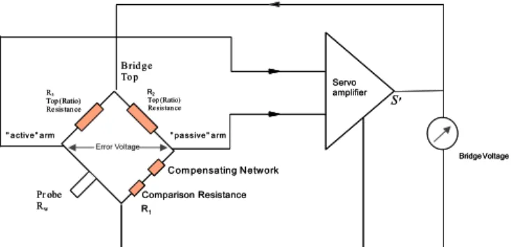
Implementation of the Constant Temperature Anemometer
The velocity is measured by its cooling effect on a heated sensor. A feedback loop in the electronics keeps the sensor temperature constant under all flow conditions. The voltage drop across the sensor thus becomes a direct measure of the power dissipated by the sensor. The anemometer output therefore represents the instantaneous velocity in the flow. Sensors are normally thin wires with diameters down to a few micrometers. The small thermal inertia of the sensor in combination with very high servo-loop amplification makes it possible for the CTA to follow flow fluctuations up to several hundred kHz. shows a basic diagram of a Constant Temperature Anemometer
" a ctive " a rm " p a ss ive " a rm R2
Top Ratio sis ce
( ) Re tan
C om pensating N etw ork
Comparison Resistance R1
Servo amplifier
c
S
Pr obe Rw
Voltage Bridge B rid g e
To p
R Top Ratio
sis ce
3
( ) Re tan
" a ctive " a rm " p a ss ive " a rm R2
Top Ratio sis ce
( ) Re tan
C om pensating N etw ork
Comparison Resistance R1
Servo amplifier
c
S
Pr obe Rw
Voltage Bridge B rid g e
To p
R Top Ratio
sis ce
3
( ) Re tan
The relationship between the fluid velocity and the heat loss of a cylindrical wire is based on the assumption that the fluid is incompressible and that the flow around the wire is potential. When a current is passed through wire, heat is generated (I2Rwire). During equilibrium, the heat generated is balanced by the heat loss (primarily convective) to the surroundings. If the velocity changes, then the convective heat transfer coefficient will also change resulting in a wire temperature change that will eventually reach a new equilibrium with the surroundings.
The heat transfer equations governing the behavior of the heated sensor includes fluid properties (heat conductivity, viscosity, density, concentration, etc.), as well as temperature loading, sensor geometry and flow direction with respect to the sensor. Thus, the multi dependency of the CTA makes it possible to measure other fluid parameters, such as concentration, and provide the ability to decompose the velocity vector into its components.
Governing Equation:
Consider a thin heated wire mounted to supports and exposed to a velocity U.
dt
i
dQ
Q
W
. (2)W = power generated by Joule heating W = I2 Rw , recall Rw = Rw(Tw) Q = heat transferred to surroundings Qi = CwTw =thermal energy stored in wire Cw = heat capacity of wire
Tw = wire temperature
The voltage-velocity relation has an exponential nature, which makes it strongly non-linear, but results in a nearly constant relative sensitivity over very large velocity ranges. The CTA, therefore, covers velocities from a few cm/s to well above the speed of sound.
The complexity of the transfer function makes it mandatory to calibrate the anemometer before use. In 2 -and 3-dimensional flow measurements, directional calibrations must be performed in addition to the velocity calibration.
The CTA anemometer is ideally suited for the measurement of time series in one-, two- or three-dimensional flows, where high temporal and spatial resolution is required. It requires no special preparation of the fluid (seeding or the like) and can measure in places not readily accessible thanks to small probe dimensions.
CTA Sensors and Their Characteristics
Anemometer probes are available with four types of sensors: Miniature wires, Gold-plated wires, Fiber-film or Film-sensors. Wires are normally 5 m in diameter and 1.2 mm long suspended between two needle-shaped prongs. Gold-plated wires have the same active length but are copper- and gold-plated at the ends to a total length of 3 mm long in order to minimize prong interference. Fiber-sensors are quartz-fibers, normally 70 mm in diameter and with 1.2 mm active length, covered by a nickel thin-film, which again is protected by a quartz coating. Fiber-sensors are mounted on prongs in the same arrays, as are wires. Film-sensors consist of nickel thin-films deposited on the tip of aerodynamically shaped bodies, wedges or cones. CTA anemometer probes may be divided in to four categories
Sensor Type Selection
Figure 3. CTA sensors. From top left going clock wise: Wire sensor, Gold plated wire sensor, Fiber film sensor and Film sensor.
Wire Sensors
Miniature wires:
First choice for applications in air flows with turbulence intensities up to 5-10%. They have the highest frequency response. Repairable.
Gold-plated wires:
For applications in airflows with turbulence intensities up to 20-25%. Repairable.
Film-Film Sensors
Thin-quartz coating:
For applications in air. Frequency response is inferior to wires. They are more rugged than wire sensors and can be used in less clean air. Repairable.
Heavy-quartz coating:
For applications in water. Repairable.
Film-Sensors
Thin-quartz coating:
For applications in air at moderate-to-low fluctuation frequencies. They are the most rugged CTA probe type and can be used in less clean air than fiber-sensors. Not repairable.
Heavy-quartz coating:
For applications in water. They are more rugged than fiber-sensors. Not repairable.
CTA Sensor Arrays
Probes are available in one-, two- and three-dimensional versions as single-, dual and triple-sensor probes referring to the number of sensors. Since the sensors (wires or fiber-films) respond to both magnitude and direction of the velocity vector, information about both can be obtained, only when two or more sensors are placed under different angles to the flow vector.
Sensor Array Selection
Figure 4. CTA sensor arrays. From Top left going clock wise: Single wire sensor, Dual wire sensor and Triple wire sensor.
Single-Sensor Normal Probes
For one-dimensional, uni-directional flows. They are available with different prong geometry, which allows the probe to be mounted correctly with the sensor perpendicular and prongs parallel with the flow.
Single-sensor slanted probes (45° between sensor and probe axis): For three-dimensional stationary flows where the velocity vector stays within a cone of 90°. Spatial resolution 0.8x0.8x0.8 mm (standard probe). Must be rotated during measurement.
Dual-Sensor Probes
X-probes:
For two-dimensional flows, where the velocity vector stays within ±45° of the probe axis.
Split-fiber probes:
For two-dimensional flows, where the velocity vector stays within ±90° of the probe axis. The cross-wise spatial resolution is 0.2 mm, which makes them better than X-probes in shear layers.
Triple-Sensor Probes
Tri-axial probes:
For 3-dimensional flows, where the velocity vector stays inside a cone of 70° opening angle around the probe axis, corresponding to a turbulence intensity of 15%. The spatial resolution is defined by a sphere of 1.3 mm diameter.
Triple-split film probes:
For fully reversing two-dimensional flows, Acceptance angle is ±180°.
Constant Temperature Anemometer Calibration
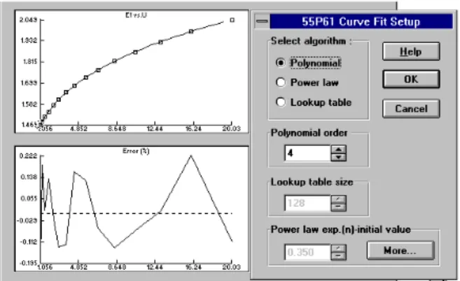
The CTA voltage output, E, has a non-linear relation with the input cooling velocity impinging on the sensor, U. Even though analytical treatment of the heat balance on the sensor shows that the transfer function has a power-law relationship of the form
(King’s Law), with constants A, B, and n, it is most often modeled using a fourth order polynomial relation. Moreover, any flow variable, which affects the heat transfer from the heated CTA sensor, such as the fluid density and temperature, affects the sensor response. Hence, CTA sensors need to be calibrated for their velocity response before use. In many cases, they also need to be calibrated for angular response. A common case such as gradually increasing ambient temperature can be dealt with either by
performing a range of velocity calibrations for the range of ambient temperatures, or by performing analytical temperature corrections for the measured voltages. Jørgensen, Dantec Dynamics A/S describes a temperature correction method, which makes it possible to reduce the influence of temperature variations on the measured velocity to typically less than +/- 0.1%/C.
n
BU A
E2
Figure 5. Typical probe calibration and curve fitting for single sensor probe.
In addition to the King’s Law response by the Hot-Wire Anemometer probe for a velocity normal to the wire, for multi wire probes the probes must also under go a YAW calibration to take into account the Cosine angular response of the wire(s) to the cooling velocity.
X-Probe Directional Calibration
Most CTA probe sensors have a pronounced directional sensitivity, especially cylindrical sensors with a large length to diameter ratios. An infinitely long cylindrical sensor has a cosine relation between the effective cooling velocity and the actual flow velocity. Finite sensors have a tangential cooling added to the cosine contribution, defined by the yaw factor k or k2.
The effective cooling velocity can be described as:
Ueff2 = U02·(cos2D + k2·sin2D) = Un2 + k2·Ut2. (3)
Where
Ueff = Effective cooling velocity U0= Actual velocity
D = angle between sensor normal and the actual velocity k = Yaw factor
Un= Velocity component perpendicular to the sensor Ut= Velocity component parallel with the sensor
The yaw factor is to some extent depending on the angle D and the velocity U0 . Yaw calibration should be performed at the velocity expected during measurements and to select a k-value that optimizes the directional response best within the expected angular range.
Typically X-array probes have configuration defaults for the yaw factors (k12 and k22 ). It is however, recommended to perform individual directional calibrations, to obtain maximum accuracy, especially in highly turbulent flows.
angle and probe voltages are recorded.
In each angular position the cooling velocity equations for the two sensors form an equation system with two unknowns, namely k1 and k2. By solving the equations, a value of k1 and k2 are obtained for each angle. The average k1 and k2 will then be used as yaw constants for the probe, when velocity decomposition are carried out in Conversion/Reduction procedures.
Tri-Axial Probe Directional Calibration
Tri-axial probes are used in 3-D flows and the directional calibration includes the pitch factor in addition to the yaw factor. The pitch factor defines how the sensor response varies, when the actual velocity vector moves out of the wire-prong plane.
The pitch factor h is defined by means of the expression:
U eff
2 = U
0 2
·(cos2T + h2·sin2T) = Un 2
+ h2·Ubn 2
. (4)
Where U
eff = Effective cooling velocity U
0= Actual velocity
T= angle between sensor-prong plane and actual velocity vector h= Pitch factor
Un = Velocity component perpendicular to the sensor (in the sensor/prong plane)
Ubn = Velocity component perpendicular to the sensor/prong plane
Tri-axial probes normally have configuration defaults for both yaw and pitch factors (k2 and h2 ). It is however, recommended to perform individual directional calibrations, if you want to obtain maximum accuracy, especially in highly turbulent flows.
Directional calibrations require that the probe is placed in a rotating holder in a plane flow field of constant velocity. The probe is then set to a fixed inclination angle and rotated through 360q around the probe axis, while related values of roll angle and probe voltages are recorded.
In each angular position the cooling velocity equation for the each sensor forms an equation system with two unknowns, namely k2 and h2. By solving the equations, values of ki
2 and hi
2
(i = 1,2,3) are obtained for each angle. The average ki
2
and hi2 will then be used as yaw and pitch constants for the probe..
Dealing With Multiple Wire Probes
Dual-Sensor (X-Array) Probes.
Figure 6. X-wire wire coordinate system.
Dual sensor probes (X-probes) have the sensor plane in the xy-plane of the probe coordinate system. The angle between the x-axis and wire 1 is denoted D(x/1) and between the x-axisD(x/2).
Velocity Decomposition:
Figure 7. X-wire probe coordinate system.
In StreamWare the following equations are used for calculation the velocity components (W is zero or can be neglected) on basis of the calibration velocities and the yaw-factors k1, k2 for the wires. The following steps are carried out:
Calibration velocity (U1cal,U2cal) to Wire coordinate system (U1,U2):
U
1cal2·(1+k
12)·cos(90-
D
(x/1)) = k
12·U
12+ U
22U
2cal2·(1+k
22)·cos(90-
D
(x/2))
2= U
12+ k
22·U
22.
(5)These two equations are solved with respect to U1 and U2 and inserted in the Wire (U1,U2) to Probe (U,V) coordinate equations:
U = U1·cosD1 + U2·cosD2
V = U·1sinD1 -U2·sinD2. (6)
Tri-Axial Probes:
Figure 8. Triple-wire probe coordinate system.
The probe is placed in a three-dimensional flow with the probe axis aligned with the main flow vector.
The velocity components U, V and W in the probe coordinate system (x,y,z) are given by:
U = U
1·cos54.736
q
+ U
2·cos54.
q
736
q
+ U
3·cos54.736
q
V = -U
1·cos45
q
- U
2·cos135
q
+ U
3·cos90
q
W = -U1·cos114.094q - U2·cos114.094q - U3·cos35.264q. (7)
Where U1, U2 and U3 are calculated from the general set of equations:
U1eff 2
= k1 2
·U1 2
+ U2 2
+ h1 2
·U3 2 U2eff
2 = h2
2 ·U1
2 + k2
2 ·U2
2 + U3
2 U3eff
2 = U1
2 + h3
2 ·U2
2 + k3
2
Where U1eff , U2eff and U3eff are the effective cooling velocities acting on the three sensors and ki and hi are the yaw and pitch factors, respectively.
As Tri-axial probes are calibrated with the velocity in direction of the probe axis Ueff is replaced by Ucal·(1+ki2+hi2)
0.5
·cos54.736q,
where 54.736q is the angle between the velocity and the wires:
U1cal2·(1+k12+h12) · cos254.736q= k12·U12 + U22 + h12·U32 U2cal2·(1+k22+h22)· cos254.736q= h22·U12 + k22·U22 + U32 U3cal2·(1+k32+h32)· cos254.736q = U12 + h32·U22 + k32·U32. (9) With the default values k2 = 0.0225 and h2 = 1.04 the solution for U1, U2 and U3 becomes:
U1=(-0.3477·U1cal2+0.3544·U2cal2+0.3266·U3cal2 )0.5 U2=(0.3266·U2cal2-0.3477·U2cal2+0.3544·U3cal2 )0.5
U3=(0.3544·U1cal2+0.3266·U2cal2-0.3477·U3cal2 )0.5. (10)
Commercial Hot-Wire Anemometers
Figure 9. Typical modern CTA configuration.
Modern Constant Temperature Anemometer systems are typically comprised of three elements.
1. A computer with an Analog to Digital converter and data acquisition software for sampling the analog signal from the Constant Temperature Anemometer and performing some degree of digital signal processing.
2. The Constant Temperature Anemometer, which should provide the user with a range of configuration options. It should be possible to modify resistor configuration for the bridge top (see), since this resistor configuration will influence the maximum heat transfer from a probe for a given application and moreover, the frequency response of the system. Signal conditioning electronics should be present. Typical signal conditioning options are: Signal amplification (gain) typically used in conjunction with turbulence measurements and to match the CTA signal to the digital sampling unit. High and low pass filters to prevent aliasing when digitally sampling the analog CTA signal and to filter out DC signal components to allow high gain turbulence measurements. Input offset to eliminate V0 (the anemometer output signal at zero velocity).
3. A calibration facility that covers a wide velocity range. Water calibration system typically has a velocity range from a few cm/sec to 10 m/s. Gas calibration system typically has velocity range spanning from a few cm/sec at the lower end going up to MACH 1.
Laser Doppler Anemometry (LDA)
Laser Doppler Anemometry is a non-intrusive technique used to measure the velocity of particles suspended in a flow. If these
particles are small, in the order of microns, they can be assumed to be good flow tracers following the flow and thus their velocity corresponds to the fluid velocity. Important characteristics of the LDA technique, listed in the following section, make it an ideal tool for dynamic flow measurements and turbulence characterization.
Characteristics of LDA
Laser anemometers offer unique advantages in comparison with other fluid flow instrumentation:
Non-Contact Optical Measurement
Laser anemometers probe the flow with focused laser beams and can sense the velocity without disturbing the flow in the measuring volume. The only necessary conditions are a transparent medium with a suitable concentration of tracer particles (or seeding) and optical access to the flow through windows, or via a submerged optical probe. In the latter case the submerged probe will of course to some extent disturb the flow, but since the measurement take place some distance away from the probe itself, this disturbance can normally be ignored.
No Calibration - No Drift
The laser anemometer has a unique intrinsic response to fluid velocity - absolute linearity. The measurement is based on the stability and linearity of optical electromagnetic waves, which for most practical purposes can be considered unaffected by other physical parameters such as temperature and pressure.
Well-Defined Directional Response
The quantity measured by the laser Doppler method is the projection of the velocity vector on the measuring direction defined by the optical system (a true cosine response).The angular response is thus unambiguously defined.
High Spatial and Temporal Resolution
The optics of the laser anemometer are able to define a very small measuring volume and thus provides good spatial resolution and yield a local measurement of Eulerian velocity. The small measuring volume, in combination with fast signal processing electronics, also permits high bandwidth, time-resolved measurements of fluctuating velocities, providing excellent temporal resolution. Usually the temporal resolution is limited by the concentration of seeding rather than the measuring equipment itself.
Multi-Component Bi-Directional Measurements
Combinations of laser anemometer systems with component separation based on color, polarization or frequency shift allow one-, two- or three-component LDA systems to be put together based on common optical modules. Acousto-optical frequency shift allows measurement of reversing flow velocities.
Principles of LDA
Laser Beam
core-intensity. At one point the cross section attains its smallest value, and the laser beam is uniquely described by the size and position of this so-called beam waist.
With a known wavelength O of the laser light, the laser beam is uniquely described by the size d0 and position of the beam waist as shown in Figure 10. With z describing the distance from the beam waist, the following formulas apply:
Figure 10. Laser beam with Guassian intensity distribution.
Beam divergence
0
4 d
S O
D (11)
Beam diameter ¸¸ o of
¹ · ¨ ¨ © §
z z
d z d
z
d( ) 1 4 for
2
2 0
0 D
S O
(12)
Wave front radius
¯ ®
f o o
o f o
» » » ¼ º
« « « ¬ ª
¸ ¸ ¹ · ¨ ¨ © §
z z
z z
d z z R
for 0 for 4
1 ) (
2 2 0
O S
(13)
The beam divergenceD is much smaller than indicated in Figure
10, and visually the laser beam appears to be straight and of constant thickness. It is important however to understand, that this is not the case, since measurements should take place in the beam waist to get optimal performance from any LDA-equipment. This is due to the wave fronts being straight in the beam waist and curved elsewhere. According to the previous equations, the wave front radius approaches infinity for z approaching zero, meaning that the wave fronts are approximately straight in the immediate vicinity of the beam waist, thus letting us apply the theory of plane waves and greatly simplify calculations.
Doppler Effect
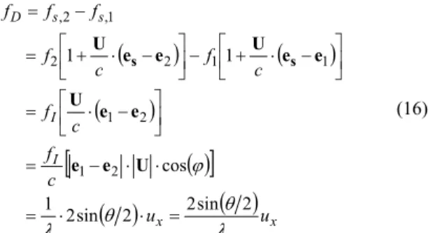
Laser Doppler Anemometry utilizes the Doppler effect to measure instantaneous particle velocities. When particles suspended in a flow are illuminated with a laser beam, the frequency of the light scattered (and/or refracted) from the particles is different from that of the incident beam. This difference in frequency, called the Doppler shift, is linearly proportional to the particle velocity.
Figure 11. Light scattering from a moving seeding particle.
The principle is illustrated in Figure 11 where the vector U represents the particle velocity, and the unit vectors ei and es describe the direction of incoming and scattered light respectively. According to the Lorenz-Mie scattering theory, the light is scattered in all directions at once, but we consider only the light reflected in the direction of the LDA receiver. The incoming light has the velocity c and the frequency fi, but due to the particle movement, the seeding particle “sees” a different frequency, fs, which is scattered towards the receiver. From the receiver’s point of view, the seeding particle acts as a moving transmitter, and the movement introduces additional Doppler-shift in the frequency of the light reaching the receiver. Using Doppler-theory, the frequency of the light reaching the receiver can be calculated as:
cc f
f
s i s
/ 1
/ 1
U e
U ei
(14)
Even for supersonic flows the seeding particle velocity U is much lower than the speed of light, meaning that U/c1. Taking advantage of this, the above expression can be linearized to:
f fc f f c
f
fs# i«¬ª1Ueseiº»¼ i iUesei i' (15)
With the particle velocity U being the only unknown parameter, then in principle the particle velocity can be determined from measurements of the Doppler shift'f.
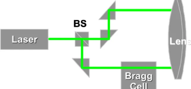
In practice this frequency change can only be measured directly for very high particle velocities (using a Fabry - Perot interferometer). This is why in the commonly employed fringe mode, the LDA is implemented by splitting a laser beam to have two beams intersect at a common point so that light scattered from two intersecting laser beams is mixed, as illustrated in Figure 12. In this way both incoming laser beams are scattered towards the receiver, but with slightly different frequencies due to the different angles of the two laser beams. When two wave trains of slightly different frequency are super-imposed we get the well-known phenomenon of a beat frequency due to the two waves intermittently interfering with each other constructively and destructively. The beat frequency corresponds to the difference between the two wave-frequencies, and since the two incoming waves originate from the same laser, they also have the same frequency,f1=f2=fI, where the subscript “I” refers to the incident light:
Laser
Laser
Bragg
Bragg
Cell
Cell
BS
Lens
Lens
Laser
Laser
Bragg
Bragg
Cell
Cell
BS
Lens
Lens
Figure 12. LDA Set-up – left schematic shows beam-splitter
>
@
x x I I s s D u u c f c f c f c f f f f O T T O M 2 sin 2 2 sin 2 1 cos 1 1 2 1 2 1 1 1 2 2 1 , 2 , »¼ º «¬ ª »¼ º «¬ª
»¼ º «¬
ª
U e e e e U e e U e e U s s (16)
whereT is the angle between the incoming laser beams and M is the angle between the velocity vector U and the direction of measurement. Note that the unit vector es has dropped out of the calculation, meaning that the position of the receiver has no direct influence on the frequency measured. (According to the Lorenz-Mie light scattering theory, the position of the receiver will however have considerable influence on signal strength). The beat-frequency, also called the Doppler-frequency fD, is much lower than the frequency of the light itself, and it can be measured as fluctuations in the intensity of the light reflected from the seeding particle. As shown in the previous equation the Doppler-frequency is directly proportional to the x-component of the particle velocity, and thus can be calculated directly fromfD:
D x f u 2 sin 2 T O (17)
Further discussion on LDA theory and different modes of
operation may be found in the classic texts of Durst et al
(1976) and Watrasiewics and Rudd (1976) and the more
resent Albrecht, Borys, Damaschke and Tropea: Laser
Doppler and Phase Doppler Measurement Techniques
(2003), ISBN 3-540-67838-7, Springer Verlag
Calibration
The LDA measurement principle is given by the relationVx= df
x fd whereVx is the component of velocity in the plane of the laser
beams, and perpendicular to their bisector, df is the distance
between fringes, and fdis the Doppler frequency. The fringe spacing
is a function of the distance between the two beams on the front lens and the focal length of the lens, given by the relation df =O/>2sin
(T/2)@ whereO = laser wavelength and T = beam crossing angle. Sincedfis a constant for a given optical system, there is a linear
relation between the Doppler frequency and velocity. The calibration factor, i.e. the fringe spacing, is constant, calculable from the optical parameters, and mostly unaffected by other changing variables in the experiment. Hence, the LDA requires no physical calibration prior to use.
Implementation
The Fringe Model
Although the above description of LDA is accurate, it may be intuitively difficult to quantify. To handle this, the fringe model is commonly used in LDA as a reasonably simple visualization producing the correct results.
When two coherent laser beams intersect, they will interfere in the volume of the intersection. If the beams intersect in their respective beam waists, the wave fronts are approximately plane, and consequently the interference will produce parallel planes of light and darkness as shown in Figure 13.The interference planes are
known as fringes, and the distanceįf between them depends on the wavelength and the angle between the incident beams:
x
z
x
z
Figure 13. Fringes at the point of intersection of two coherent beams.
2 sin 2 T
O
Gf (18)
The fringes are oriented normal to the x-axis, so the intensity of light reflected from a particle moving through the measuring volume will vary with a frequency proportional to thex-component,ux, of the particle velocity:
x f x D u u f O T G 2 sin 2 (19)
If the two laser beams do not intersect at the beam waists but elsewhere in the beams, the wave fronts will be curved rather than plane, and as a result the fringe spacing will not be constant but depend on the position within the intersection volume. As a consequence, the measured Doppler frequency will also depend on the particle position, and as such it will no longer be directly proportional to the particle velocity, hence resulting in a velocity bias.
Measuring Volume
Measurements take place in the intersection between the two incident focused laser beams, and the measuring volume is defined as the volume within which the modulation depth is higher than e-2 times the peak core value. Due to the Gaussian intensity distribution in the beams the measuring volume is an ellipsoid as indicated in Figure 14
.
Figure 14. LDA measurement volume.
width:
L y
D E
F
S O
G 4 (21)
height:
¸ ¹ · ¨ © §
2 cos 4
T S
O G
L x
D E
F
(22)
where F is the lens’ focal length, E is the beam expansion (see Figure 15), andDL is the initial beam thickness (e-2).
F
D
u
E
-u
(
D
D
L
F
D
u
E
-u
(
D
D
L
Figure 15. shows the use of a beam expander to increase beam separation priorto focusing at a common point.
As important are the fringe separation and number of fringes in the measurement volume. These are given by:
fringe separation:
¸ ¹ · ¨ © §
2 sin
2 T
O
Gf (23)
Number of fringes:
L f
D E F N
S T¸
¹ · ¨ © §
2 tan 8
(24)
This number of fringes applies for a seeding particle moving straight through the center of the measuring volume along the x-axis. If the particle passes through the outskirts of the measuring volume, it will pass fewer fringes, and consequently there will be fewer periods in the recorded signal from which to estimate the Doppler frequency. To get good results from the LDA-equipment, one should ensure a sufficiently high number of fringes in the measuring volume. Typical LDA set-ups produce between 10 and 100 fringes, but in some cases reasonable results may be obtained with less, depending on the electronics or technique used to determine the frequency. The key issue here is the number of periods produced in the oscillating intensity of the reflected light, and while modern processors using FFT technology can estimate particle velocity from as little as one period, the accuracy will improve with more periods.
Backscatter Versus Forward Scatter
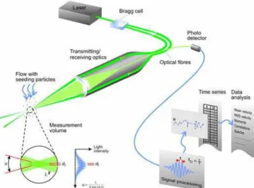
A typical LDA setup in the so-called back-scatter mode is shown in Figure 16. The figure also shows the important components of a modern commercial LDA system. The majority of light from commonly used seeding particles is scattered in a direction away from the transmitting laser, and in the early days of LDA, forward scattering was thus commonly used, meaning that the receiving optics was positioned opposite of the transmitting aperture (consult text by van den Hulst, 1981, for discussion on light scattering).
Figure 16. Schematic of components for a modern back-scatter LDA system.
180 0
90
270 210 150
240 120
300 60
330 30
dp#0.2O
180 0
330 210
240 300
270 150
120 90
60
30
dp#1.0O
180 0
210 150
240 120
270 90
60
300 30
330
dp#10O
Figure 17. Mie scatter diagram for different size seeding particles dp is particle size.
Figure 17 shows the mie scatter function for three different particle sizes. From the left size<O, center size=Oand right size>O.
Most LDA measurements are performed using seeding particles that are larger than the wave length of the laser light of most lasers. Figure 17 illustrates that a much smaller amount of light is scattered back towards the transmitter, but advances in technology has made it possible to make reliable measurements even on these faint signals, and today backward scatter is the usual choice in LDA. This so-called backscatter LDA allows for the integration of transmitting and receiving optics in a common housing (as seen in Figure 16), saving the user a lot of tedious and time-consuming work aligning separate units.
Forward scattering LDA is however, not completely obsolete since in some cases the improved signal-to-noise ratio make forward-scatter the only way to obtain measurements at all. Experiments requiring forward scatter might include:
High speed flows, requiring very small seeding particles, which stay in the measuring volume for a very short time, and thus receive and scatter a very limited number of photons.
Transient phenomena which require high data-rates in order to collect a reasonable amount of data over a very short period of time.
Very low turbulence intensities, where the turbulent fluctuations might drown in noise, if measured with backscatter LDA.
measuring volume, and in many cases also disturbs measurements near surfaces due to reflection of the laser beams.
Figure 18. Off-axis scattering.
Figure 18 illustrates how off-axis scattering reduces the effective size of the measuring volume. Seeding particles passing through either end of the measuring volume will be ignored since they are out of focus, and as such contribute to background noise rather than to the actual signal. This reduces the sensitivity to velocity gradients within the measuring volume, and the off-axis position of the receiver automatically reduces problems with reflection. These properties make off-axis scattering LDA very efficient for example in boundary layer or near- surface measurements.
Optics
In modern LDA equipment the light from the beam splitter and the Bragg cell is sent through optical fibers, as is the light scattered back from seeding particles. This reduces the size and the weight of the probe itself, making the equipment flexible and easier to use in practical measurements. A photograph of a pair of commercially available LDA probes is shown in Figure 19. The laser, beam splitter, Bragg cell and photodetector (receiver) can be installed stationary and out of the way, while the LDA-probe can be traversed between different measuring positions.
Figure 19. Photograph of modern commercial fiber optic based LDA probes.
It is normally desired to make the measuring volume as small as possible, which according to the formulas governing the measurement volume means that, the beam waist
L f
ED F d
S O
4
(25)
should be small. The laser wavelength O is a fixed parameter, and focal length F is normally limited by the geometry of the model being investigated. Some lasers allow for adjustment of the beam waist position, but the beam waist diameterDL is normally fixed. This leaves beam expansion as the only remaining way to reduce the
size of the measuring volume. When no beam expander is installed, thenE= 1.
A beam expander is a combination of lenses in front of or replacing the front lens of a conventional LDA system. It converts the beams exiting the optical system to beams of greater width. At the same time the spacing between the two laser beams is increased, since the beam expander also increases the aperture. Provided the focal length F remains unchanged, the larger beam spacing will thus increase the angle T between the two beams. According to the formulas in governing the measurement volume this will further reduce the size of the measuring volume.
In agreement with the fundamental principles of wave theory, a larger aperture is able to focus a beam to a smaller spot size and hence generate greater light intensity from the scattering particles. At the same time the greater receiver aperture is able to pick up more of the reflected light. As a result the benefits of the beam expander are threefold:
x Reduce the size of the measuring volume at a given measuring distance.
x Improve signal-to-noise ratio at a given measuring distance, or
x Reach greater measuring distances without sacrificing signal-to-noise.
Frequency Shift
A drawback of the LDA-technique described so far is that negative velocitiesux< 0 will produce negative frequenciesfD < 0. However, the receiver can not distinguish between positive and negative frequencies, and as such, there will be a directional ambiguity in the measured velocities.
To handle this problem, a Bragg cell is introduced in the path of one of the laser beams (as shown in Figure 12). The Bragg cell shown in Figure 20 is a block of glass. On one side, an electro-mechanical transducer driven by an oscillator produces an acoustic wave propagating through the block generating a periodic moving pattern of high and low density. The opposite side of the block is shaped to minimize reflection of the acoustic wave and is attached to a material absorbing the acoustic energy.
Figure 20. Principles of operation of a Bragg cell.
The Bragg cell adds a fixed frequency shift f0 to the diffracted beam, which then results in a measured frequency off a moving particle of
x
D f u
f
O - 2 sin 2
0
# (26)
and as long as the particle velocity does not introduce a negative frequency shift numerically larger than f0, the Bragg cell with thus ensure a measurable positive Doppler frequencyfD. In other words the frequency shiftf0 allows measurement of velocities down to
2 sin 2
0
-Of
ux ! (27)
without directional ambiguity. Typical values might be O = 500 nm, f0 = 40 MHz, T = 20o, allowing of negative velocity components down to ux > -57.6 m/s. Upwards the maximum measurable velocity is limited only by the response-time of the photo-multiplier and the signal-conditioning electronics. In modern commercial LDA equipment, such a maximum is well into the supersonic velocity regime.
Figure 21. Resolving directional ambiguity using frequency shift.
Signal Processing
The primary result of a laser anemometer measurement is a current pulse from the photodetector. This current contains the frequency information relating to the velocity to be measured. The photocurrent also contains noise, with sources for this noise being:
x Photodetection shot noise
x Secondary electronic noise
x Thermal noise from preamplifier circuit
x Higher order laser modes (optical noise)
x Light scattered from outside the measurement volume, dirt, scratched windows, ambient light, multiple particles, etc.
x Unwanted reflections (windows, lenses, mirrors, etc). The primary source of noise is the photodetection shot noise, which is a fundamental property of the detection process. The interaction between the optical field and the photo-sensitive material is a quantum process, which unavoidably impresses a certain amount of fluctuation on the mean photocurrent. In addition there is mean photocurrent and shot noise from undesired light reaching the photodetector. Much of the design effort for the optical system is aimed at reducing the amount of unwanted reflected laser light or ambient light reaching the detector.
A laser anemometer is most advantageously operated under such circumstances that the shot noise in the signal is the predominant noise source. This shot noise limited performance can be obtained by proper selection of laser power, seeding particle size and optical system parameters. In addition, noise should be minimized by selecting only the minimum bandwidth needed for measuring the desired velocity range by setting low-pass and high-pass filters in the signal processor input. Very important for the
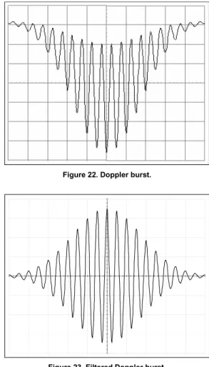
quality of the signal, and the performance of the signal processor, is the number of seeding particles present simultaneously in the measuring volume. If on average much less than one particle is present in the volume, we speak of a burst-type Doppler signal. Typical Doppler burst signals are shown in Figure 22.
Figure 22. Doppler burst.
Figure 23. Filtered Doppler burst.
Figure 23 shows the filtered signal, which is actually input to the signal processor. The DC-part, which was removed by the high-pass filter, is known as the Doppler Pedestal. The envelope of the Doppler modulated current reflects the Gaussian intensity distribution in the measuring volume.
If more particles are present in the measuring volume simultaneously, we speak of a multi-particle signal. The detector current is the sum of the current bursts from each individual particle within the illuminated region. Since the particles are located randomly in space, the individual current contributions are added with random phases, and the resulting Doppler signal envelope and phase will fluctuate. Most LDA-processors are designed for single-particle bursts, and with a multi-single-particle signal, they will normally estimate the velocity as a weighted average of the particles within the measuring volume. One should be aware however, that the random phase fluctuations of the multi-particle LDA signal adds a phase noise to the detected Doppler frequency, which is very difficult to remove.
^
`
2 1 0 2 / 2 exp ¦ N n nk x j kn N
S S (28)
whereNis the number of discrete samples, andK = -N, -N+ 1, …, N – 1. The Doppler frequency is given by the peak of the spectrum.
Data Analysis
In LDA there are two major problems faced when making a statistical analysis of the measurement data; velocity bias and the random arrival of seeding particles to the measuring volume. While velocity bias is the predominant problem for simple statistics, such as mean and rms values, the random sampling is the main problem for statistical quantities that depend on the timing of events, such as spectrum and correlation functions (see Lee & Sung, 1994).
Table 2 illustrates the calculation of moments, on the basis of measurements received from the processor. The velocity data coming from the processor consists of N validated bursts, collected during the time T, in a flow with the integral time scaleWI. For each burst the arrival timeai and the transit timetiof the seeding particle is recorded along with the non-cartesian velocity components (ui,vi,
wi). The different topics involved in the analysis are described in more detail in the open literature, and will be touched upon briefly in the following section.
Making Measurements
Dealing With Multiple Probes (3D Setup)
The non-cartesian velocity components (u1, u2, u3) are transformed to cartesian coordinates (u, v, w) using the transformation matrixC:
° ¿ ° ¾ ½ ° ¯ ° ® ° ¿ ° ¾ ½ ° ¯ ° ® ° ¿ ° ¾ ½ ° ¯ ° ® 3 2 1 33 32 31 23 22 21 13 12 11 u u u C C C C C C C C C w v u (29)
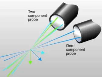
A typical 3-D LDA setup requiring coordinate transformation is shown in Figure 24, where 3-dimensional velocity measurements are performed with a 2-D probe positioned at off-axis angle D1 and a 1-D probe positioned at off-axis angleD2. The transformation for this case is: ° ¿ ° ¾ ½ ° ¯ ° ® ° ° ° ¿ ° ° ° ¾ ½ ° ° ° ¯ ° ° ° ® ° ¿ ° ¾ ½ ° ¯ ° ® 3 2 1 2 1 1 2 1 2 2 1 1 2 1 2 ) sin( cos ) sin( cos 0 ) sin( sin ) sin( sin 0 0 0 1 u u u w v u D D D D D
D D D
D D
D
D (30)
Figure 24. Typical 3-D LDA setup requiring coordinate transformation.
Buchave, in DISA Information No. 29 shows demonstrates that to obtain a good accuracy for the transformed V and W velocity components the minimum angle between the to incident fringe sets should be no less than 19 deg,
Calculating Moments
Moments are the simplest form of statistics that can be calculated for a set of data. The calculations are based on individual samples, and the possible relations between samples are ignored as is the timing of events. This leads to moments sometimes being referred to as one-time statistics, since samples are treated one at a time.
Table 2 lists the formulas used to estimate the moments. The table operates with velocity-components xi and yi, but this is just examples, and could of course be any velocity component, cartesian or not. It could even be samples of an external signal representing pressure, temperature or something else.
Table 2. Estimation of moments.
Mean ¦1
0
N
i i i
u u K Variance 2 1 0
2 N¦
i i i
u u
K V
RMS V V2
Turbulence 100%
u Tu V Skewness 3 1 0 3 1 ¦ N
i i i
u u S K V Flatness 4 1 0 4 1 ¦ N
i i i
u u
F K
V
Cross-Moments uv uv N
u u vi v
i i i
¦1
0
K
Velocity Bias and Weighting Factor
Even for incompressible flows where the seeding particles are statistically uniformly distributed, the sampling process is not independent of the process being sampled (that is the velocity field). Measurements have shown that the particle arrival rate and the flow field are strongly correlated ([McLaughlin & Tiedermann (1973)] and [Erdmann & Gellert (1976)]). During periods of higher velocity, a larger volume of fluid is swept through the measuring volume, and consequently a greater number of velocity samples will be recorded. As a direct result, an attempt to evaluate the statistics of the flow field using arithmetic averaging will bias the results in favor of the higher velocities.
There are several ways to deal with this issue:
Ensure statistically independent samples - the time between bursts must exceed the integral time-scale of the flow field at least by a factor of two. Then the weighting factor corresponds to the
arithmetic mean, N
i
1
K . Statistically independent samples can be accomplished by using very low concentration of seeding particles in the fluid.
Use dead-time mode - The dead-time is a specified period of time after each detected Doppler-burst, during which further bursts will be ignored. Setting the dead-time equal to two time the integral time scale will ensure statistically independent samples, while the integral time-scale itself can be estimated from a previous series of velocity samples, recorded with the dead-time feature switched off.
Use bias correction - If one plans to calculate correlations and spectra on the basis of measurements performed, the resolution achievable will be greatly reduced by the low data-rates required to ensure statistically independent samples. To improve the resolution of the spectra, a higher data rate is needed, which as explained above will bias the estimated average velocity. To correct this velocity-bias, a non-uniform weighting factor is introduced:
¦1
0
N
j j
i i
t t
K (31)
The bias-free method of performing the statistical averages on individual realizations uses the transit time, ti , weighting (see George, 1975). Additional information on the transit time weighting method can be found in [George (1978)], [Buchhave, George & Lumley (1979)] and [Buchhave (1979), Benedict & Gould (1999)]. In the literature transit time is sometimes referred to as residence time.
Particle Image Velocimetry (PIV)
Principles of PIV
PIV is a velocimetry technique based on images of tracer “seeding” particles suspended in the flow. In an ideal situation, these particles should be perfect flow tracers, homogeneously distributed in the flow, and their presence should not alter the flow properties. In that case, local fluid velocity can be measured by measuring the fluid displacement (see Figure 25) from multiple particle images and dividing that displacement by the time interval between the exposures. To get an accurate instantaneous flow velocity, the time between exposures should be small compared to the time scales in the flow, and the spatial resolution of the PIV sensor should be small compared to the length scales in the flow.
>
@
* * * *
D X t t u X t t dt t
t
( ; ,c cc |) ( ), c cc
³
* Xi( )t2
* Xi( )t1
* D
Particle trajectory
Fluid pathline * *
u X t( , ) *
v ti( )
After: Adrian,Adv. Turb. Res.(1995) 1-19
* Xi( )t2
* Xi( )t1
* D
Particle trajectory
Fluid pathline * *
u X t( , ) *
v ti( )
After: Adrian,Adv. Turb. Res.(1995) 1-19
Figure 25. Determination of particle displacement and its relationship to actual fluid velocity.
Principles of PIV have been covered in many papers including Willert C. E., and Gharib, M., (1991), Adrian, R. J., (1991) and Lourenco, L. M. et. al. (1989). A more recent book by Raffel, M., Willert, C., Kompenhans, J., (1998) is an excellent source of information on various aspects of PIV.
Figure 26. Principal layout of a PIV system.
The principle layout of a modern PIV system is shown in Figure
26. The PIV measurement includes illuminating a cross section of the seeded flow field, typically by a pulsing light sheet, recording multiple images of the seeding particles in the flow using a camera located perpendicular to the light sheet, and analyzing the images for displacement information.
The recorded images are divided into small sub-regions called interrogation regions, the dimensions of which determine the spatial resolution of the measurement. The interrogation regions can be adjacent to each other, or more commonly, have partial overlap with their neighbors. The shape of the interrogation regions can deviate from square to better accommodate flow gradients. In addition, interrogation areas A and B, corresponding to two different exposures, may be shifted by several pixels to remove a mean dominant flow direction (DC offset) and thus improve the evaluation of small fluctuating velocity components about the mean.
The peak of the correlation function gives the displacement information. For double or multiple exposed single images, an auto-correlation analysis is performed. For single exposed double images, a cross-correlation analysis gives the displacement information.
Image Processing
Figure 27. Multiple exposure image captured for PIV autocorrelation analysis.
This analysis technique has been developed for photography-based PIV, since it is not possible to advance the film fast enough between the two exposures. The auto-correlation function of a double exposed image has a central peak, and two symmetric side peaks, as shown in Figure
28
. This poses two problems: (1) although the particle displacement is known, there is an ambiguity in the flow direction, (2) for very small displacements, the side peaks can partially overlap with the central peak, limiting the measurable velocity range.Double-exposure image
Interrogation region
Spatial correlation
RP
RD+
R
D-Figure 28. Autocorrelation analysis of a double-exposed image.
In order to overcome the directional ambiguity problem, image shifting techniques using rotating mirrors (Landreth, C. C. et. al, 1988) and electro-optical techniques (Landreth, C. C. et. al. 1988), (Lourenco, L. M., 1993) have been developed. To leave enough room for the added image shift, larger interrogation regions are used for auto-correlation analysis. By displacing the second image at least as much as the largest negative displacement, the directional ambiguity is removed. This is analogous to frequency shifting in LDA systems to make them directionally sensitive. Image shifting by rotating mirrors does however, introduce a parallax error in the resulting velocity estimations. This error has been documented to be as large as 11%.
The preferred method in PIV is to capture two images on two separate frames, and perform correlation analysis. This cross-correlation function has a single peak, providing the magnitude and direction of the flow without ambiguity.
Figure 29. Auto-correlation (left) versus Cross-correlation (right) analysis result.
Common particles need to exist in the interrogation regions, which are being correlated, otherwise only random correlation, or noise will exist. The PIV measurement accuracy and dynamic range increase with increasing time difference 't between the pulses. However, as't increases, the likelihood of having common particles in the interrogation region decreases and the measurement noise goes up. A good rule of thumb is to insure that within time't, the in-plane components of velocity Vx and Vy carry the particles no
more than a third of the interrogation region dimensions, and the out-of-plane component of velocityVz carries the particles no more
than a third of the light sheet thickness.
Most commonly used interrogation region dimensions are 64 by 64 pixels for auto-correlation, and 32 by 32 pixels for cross-correlation analysis. Since the maximum particle displacement is about a third of these dimensions, to achieve reasonable accuracy and dynamic range for PIV measurements, it is necessary to be able to measure the particle displacements with sub-pixel accuracy.
FFT techniques are used for the calculation of the correlation functions. Since the images are digitized, the correlation values are found for integral pixel values, with an uncertainty of ±0.5 pixels. Different techniques, such as centroids, Gaussian, and parabolic fits, have been used to estimate the location of the correlation peak. Using 8-bit digital cameras, peak estimation accuracy of between 0.1 pixels to 0.01 pixels can be obtained. In order for sub-pixel interpolation techniques to work properly, it is necessary for particle images to occupy multiple (2-4) pixels. If the particle images are too small, i.e. around one pixel, these sub-pixel estimators do not work properly, since the neighboring values are noisy. In such a case, slight defocusing of the image improves the accuracy.