K. Kamemoto
Department of Mechanical Engineering Graduate School of Engineering Yokohama National University [email protected]On Contribution of Advanced Vortex
Element Methods Toward Virtual
Reality of Unsteady Vortical Flows in
the New Generation of CFD
The purpose of this paper is to explain the attractive applicability of the advanced vortex element methods and their contribution to the beginning of the new generation of CFD, with introduction of epoch-making application of the methods to simulation of unsteady flows around bluff bodies and virtual operation of fluid machinery. The vortex methods have been developed and applied for analysis of complex, unsteady and vortical flows in relation to problems in a wide range of industries, because they consist of simple algorithm based on physics of flow. Nowadays, applicability of the vortex element methods to various engineering problems has been developed and improved dramatically and it has become encouragingly clear that the vortex methods have so much interesting features that they provide easy-to-handle and completely grid-free Lagrangian calculation of unsteady and vortical flows without use of any RANS type turbulent models. In this paper, the mathematical background and numerical procedure of a vortex method developed by the group of the present author are briefly explained, and topics of calculated flows around bluff bodies, an oscillating airfoil, a swimming fish, virtual operation of fluid machinery (pumps and water turbines) are introduced.
Keywords: Vortex method, unsteady flows, numerical calculation, bluff body fluid dynamics, virtual operation of fluid machinery
Introduction
Although the recent progress of computational fluid dynamics is quite rapid, the numerical analysis of a higher Reynolds number flow seems still not so easy, from the viewpoint of engineering applications. The applicability of the conventional turbulence models of time-mean type seems questionable as far as unsteady separated flows are concerned. And the large eddy simulation of Eulerian type inevitably meets crucial difficulties in its application to flows of higher Reynolds number, because the scheme essentially needs fine grids to obtain reasonable resolution of turbulence structures.1
On the other hand, the vortex methods have been developed and applied for analysis of complex, unsteady and vortical flows in relation to problems in a wide range of industries, because they consist of simple algorithm based on physics of flow. Leonard (1980) summarized the basic algorithm and examples of its applications. Sarpkaya (1989) presented a comprehensive review of various vortex methods based on Lagrangian or mixed Lagrangian-Eulerian schemes, the Biot-Savart law or the vortex in cell methods. Kamemoto (1995) summarized mathematical basis of the Biot-Savart law methods. In 1999, the first International Conference on Vortex Methods was held in Kobe, Japan, in which many leading works related with different kinds of vortex methods were presented, and a book consisting of selected papers of the conference was edited by Kamemoto and Tsutahara (2000). The second International Conference on Vortex Methods was held in 2001, in Istanbul, Turkey. At the conference, many attractive papers on development or application of advanced vortex methods were presented.
As well as many finite difference methods, it is a crucial point in vortex methods that the number of vortex elements should be increased when higher resolution of turbulence structures is required, and then the computational time increases rapidly. Recently, in
Presented at ENCIT2004 – 10th Brazilian Congress of Thermal Sciences and Engineering, Nov. 29 -- Dec. 03, 2004, Rio de Janeiro, RJ, Brazil.
Technical Editor: Atila P. Silva Freire.
order to overcome the crucial point, some of leading researchers examined spatial averaging models of turbulence in high Reynolds number flows for Lagrandian large eddy simulation. Leonard and Chua (1989) proposed application of the Smagorinsky model in simulations of interaction between interlocked vortex rings and interaction between two colliding vortex rings. Mansfield et al. (1998)(1999) proposed a dynamic eddy viscosity model of subfilter-scale stresses for Lagrangian vortex element methods and applied it to simulation of collision of coaxial vortex rings. Kiya et al. (1999) carried out simulation of an impulsively started round jets by a 3-d vortex method using the Smagorinsky model. Saltara et al. (1998) simulated vortex shedding from an oscillating circular cylinder with use of turbulence modeling of Smagorinsky type in a vortex in cell method. Recently, Pereira et al. (2002) proposed a local second-order velocity structure function for calculation of local kinematic energy spectrum and applied it into simulation of vortex shedding flow about a circular cylinder by a vortex method.
On the other hand, Cotte et al (2002) recently investigated reliability of numerical analysis of turbulent structures by a vortex method of so-called vortex-in-cell method presenting a comparison of the performance of the vortex method and the spectral method in a homogeneous turbulent flow at low Reynolds number and a vortex reconnection case at a moderate Reynolds number. And it was clarified from their study that the accuracy of the vortex method in the large and intermediate scales of turbulence is good enough to yield acceptable statistics. And it was also pointed that in the under-resolved case of subcore scales, vortex methods appear to behave as accurate LES models in the sense that they avoid accumulation of energy at the end of the spectrum, without excessive dissipation in the resolved scales. Fukuda and Kamemoto (2004) newly proposed a grid-free redistribution model of 3-D core spreading method for turbulent flow analysis by a vortex method based on the Biot-Savart law, and they examined the availability of the model by applying it into the flow of inclined collision of a pair of vortex rings.
The vortex methods have been applied mostly into analysis of unsteady characteristics of fundamental flows like jets or wakes behind bluff bodies, so far. On the other hand, recently, the applicability of the vortex methods based on the Biot-Savart law has been extended to numerical prediction of unsteady and complex characteristics of various flows related with difficult engineering problems concerning flow-induced vibration, off-design operation of fluid machinery, automobile aerodynamics, and biological fluid dynamics and so on. Kamemoto and Ojima (2004) reported a study of virtual operation of fluid machinery using their advanced vortex method.
In this paper, in order to deepen discussions on the contribution of the Biot-Savart law vortex methods, attractive characteristics of the methods are described, explaining mathematical background of an advanced vortex method developed and examined up to this time by the group of the present author. And, introducing the recent works on development of turbulence models for Lagrangian vortex methods, the subjects of the vortex methods which should be solved as a tool of the Lagrangian large eddy simulation are shortly discussed. Then, examples of numerical simulation of two and three-dimensional unsteady separated flows and engineering applications are introduced.
Algorithms of the Vortex Method Based on Biot-Savart
Law
Mathematical Basis
The vortex methods are based on the Navier-Stokes equation and the continuity equation for incompressible flow which are written in vector form as follows.
u u uu 1 2
w
w Q
Ugradp grad
t (1)
0
u
div (2)
Alternative expression of the governing equations of viscous and incompressible flow gives the vorticity transport equation and pressure Poisson equation which are derived from the rotation and divergence of Navier-Stokes equations, respectively.
Z Z ZZ 2
w
w Q
u
u grad grad
t
(3)
) u u (
2p div grad
U (4)
Where u is a velocity vector. The vorticity Z is defined as
u rot
Ȧ (5)
Lagrangian expression for the vorticity transport expressed by Eq. (3) is given as
Z ZZ Q2
u grad t
d d
(6)
When a two-dimensional flow is dealt with, the first term of the right hand side in Eq. (6) disappears and so the two-dimensional vorticity transport equation is simply expressed as
Z Z Q2
t d
d (7)
In the vortex method based on the Biot-Savart law, Eq. (6) is numerically solved by the operator-splitting scheme of Chorin (1973) (1978). If the vorticity of a fluid particle at time t is written
as Z (t), we obtain an approximate expression of the change of
vorticity through convection and diffusion during a small time interval dt as follows.
dt dt
grad t
dt
t Z Z Z
Z( ) () ( )u Q 2 (8)
In Eq. (8), the second term in the right hand side is based on the three-dimensional convection and stretching of vorticity, which always becomes zero for two-dimensional flow, and the third term is the rate of viscous diffusion of vorticity. If the Reynolds number of the flow is sufficiently large, the convection term is considered much larger than the diffusion term, and thus, the third term in Eq. (8) may be neglected in the computation. Furthermore, if the high Reynolds number flow is two-dimensional, Eq. (8) is approximated by a simple equation like Z (t+dt) = Z (t) = constant. Therefore, if
we take a small sectional area ds for the fluid particle and the
vorticity is assumed constant in this area, the two-dimensional fluid particle is thought a free vortex element which transports a constant circulation ī=Zds.
On the other hand, the motion of the fluid particle at a location r
is represented by a Lagrangian form of a simple differential equation.
u r t d
d (9)
Then, the trajectory of the fluid particle over a time step dt is
approximately computed from the Adams-Bashforth method as follows.
^
t t dt`
dtt dt
t ) r() 1.5u() 0.5u( ) (
r (10)
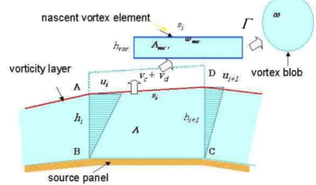
Figure 1. Flow field involving vorticity region.
Generalized Biot-Savart Law
As explained by Wu and Thompson (1973), the Biot-Savart law can be derived from integration of the vorticity definition equation expressed as Eq.(5).
^
`
³ u u
³V 0u0Gdv S (n0 u0) 0G (n0 u0) 0G ds
u Z
Here, subscript “0” denotes variable, differentiation and
integration at a location r0, and n0 denotes the normal unit vector at
a point on a boundary surface S. And G is the fundamental solution
of the scalar Laplace equation with the delta function G (r-r0) in the
right hand side, which is written as
¸ ¹ · ¨ © § R
G log 1
2 1
S (2-D) (12)
or
R G
S 4
1 (3-D) (13)
here, R=r - r0, R = |R| = | r-r0 |.
In Eq. (11), the inner product, n0x u0 and the outer product
n0uu0 stand for respectively normal and tangential velocity
components on the boundary surface, and they respectively correspond to source and vortex distributions on the surface. Therefore, as shown in Fig.1, it is mathematically understood that a velocity field of viscous and incompressible flow is arrived at the field integration concerning vorticity distributions in the flow field and the surface integration concerning source and vortex distributions around the boundary surface.
Calculation of Pressure
Instead of the finite difference calculation of the pressure Poisson equation represented by Eq. (4), the pressure in the flow field is calculated from the integration equation which was formulated by Uhlman (1992) as follows.
³ ¿ ¾ ½ ¯ ®
u
w w ³ u
³
w w
S V S G ds
t G dv G ds n G H
H ( Z) n Q n ( Z)
E u u
(14)
Here,ȕ is ȕ= 1 inside the flow and ȕ= 1/2 on the boundary S. G
is the fundamental solution given by Eq. (12) or Eq. (13), and H is the Bernoulli function defined as
2
2 u p
H
U (15)
here, u = _ u_.
Introduction of Nascent Vortex Elements
The vorticity field near the solid surface must be represented by proper distributions of vorticity layers and discrete vortex elements so as to satisfy the non-slip condition on the surface. In the advanced vortex method developed by the group of the present
author, a thin vorticity layer with thickness hi is considered along
the body surface, and the surface of the solid body is discretized by a number of source panels as shown in Fig. 2. Using normal velocity conditions on the solid surface, the strength of the source panels for the next step of calculation can be evaluated numerically from Eq. (11) by applying the panel method.
Figure 2. Thin vorticity layer and introduction of nascent vortex elements.
If the flow is considered to be two-dimensional for convenience, and a linear distribution of velocity in the thin vorticity layer is
assumed, the normal convective velocity Vc on the outer boundary
of the vorticity layer can be expressed using the relation of continuity of flow and the non-slip condition on the solid surface for the element of the vorticity layer [ABCD] as
¸ ¹ · ¨ © § 2 2
1 i i i 1 i 1
i c u h u h s
V (16)
Here, si, hi and ui respectively denote length of an outer
boundary element, vorticity layer thickness and tangential velocity at each node of the outer boundary.
On the other hand, vorticity of the thin shear layer diffuses through the outer boundary of the vorticity layer into the flow field due to viscous diffusion. In order to consider this vorticity diffusion, a diffusion velocity is employed in the same manner as the vorticity layer spreading method proposed by Kamemoto (1995), which is based on the viscous diffusion of the vorticity in the shear layer developing over a suddenly accelerated plate wall. In this case, the
displacement thickness of the vorticity layer (G ) diffuses with the
progress of time as G= 1.136(QT)1/2 from the solid surface at a time
T. Differentiating G by T and substituting the thickness of the
vorticity layer hi into G, we obtain the diffusion velocity Vd at the
outer boundary of the vorticity layer as follows.
1 2 136 1 i i d h h v
V . (17)
Here, Ȟ is kinematic viscosity of the fluid. If the value of
(Vc+Vd ) becomes positive, a nascent vortex element is introduced
in the flow field, where the thickness and vorticity of the element are given as follows.
V V dthvor c d (18)
vor vor
A
A
*
Z (19)
Here, ī is the circulation originally involved in the element of
the vorticity layer [ABCD], and A and Avor are the areas of the
vorticity layer element and the nascent vortex element.
In case of dimensional flow calculation, a three-dimensional nascent vortex element of a rectangular parallelepiped is introduced in the same manner as the two-dimensional case, through each element of the outer boundary of a thin vorticity layer. The details of treatments have been explained in the paper by Ojima and Kamemoto (2000).
It will be noteworthy that as a linear distribution of velocity is assumed in the thin vorticity layer, the shearing stress on the wall surface is evaluated approximately from the following equation as far as the thickness of the vorticity layer is sufficiently thin.
PZ P W w w y u
w (20)
Replacement with Equivalent Vortex Blobs
For simplification of numerical treatments, every nascent vortex element which is far from the solid surface can be replaced with an equivalent discrete vortex. Either in a two-dimensional flow or in a three dimensional flow, the discrete vortex element is modeled by a vortex blob which has its own smoothed vorticity distribution and a core radius, where the size of core radius spreads with time according to the viscous diffusion expressed by the third term in the right hand side of Eq. (8) as explained by Kamemoto (1995). In the present method, every nascent vortex element which moves beyond
a boundary at the distance of four times hi from the solid surface is
replaced with an equivalent and circular (2-D) or spherical (3-D) vortex blob of the core spreading model.
When a two-dimensional flow is dealt with, the total circulation and the sectional area of the blob core are determined to be the same as those of the rectangular nascent vortex element. As explained by
Leonard (1980), if a vortex blob has a core of radius İi and total
circulation īi, a Gaussian distribution of vorticity around the center
of the blob is given as
°¿ ° ¾ ½ °¯ ° ® ¸¸ ¹ · ¨¨ © § * 2 2 exp ) ( i i i
i r r
r
H SH
Z (26)
Here, ri denotes a position of the center of the blob. As
explained by Kamemoto (1995), the spreading of the core radius Hi
according to the viscous diffusion expressed by Eq. (7) is represented as i i v dt d H H 2 242 . 2 2 (27)
When a three-dimensional flow is treated, a nascent vortex element of a rectangular parallelepiped is replaced by an equivalent vortex blob with a spherically symmetric distribution of vorticity which was proposed by Winckelmans and Leonard (1988) and modified by Nakanishi and Kamemoto (1992). The details of treatments have been explained in the paper by Ojima and Kamemoto (2000). A vortex blob is a spherical model with a radially symmetric distribution of vorticity. Once the i-th vortex blob is given in a flow field by the position ri=(rx,ry,rz), its vorticity
Zi=(Zx, Zy, Zz) and its core radius Hi, the vorticity distribution
around the vortex blob is represented by the following equations.
3
( ) p(| i| / i) i dvi
L r L rr H H
Z Z (28)
Here, dvi is volume of the blob and p([) is smoothing function
proposed by Winckelmans & Leonard (1988).
2 7 2
( ) 15 8 ( 1)
p[ S [ (29)
On the other hand, the evolution of vorticity is calculated by Eq. (8) with three-dimensional core spreading method modified by Nakanishi & Kamemoto (1992). In this method, the stretch term and diffusion term of Eq. (8) are separately considered. The change
of core radius due to the stretching is calculated from the following equations.
d ( grad)
dt
Z Z
u (30)
t
t
dl l d
dt dt
Z
Z (31)
dt dl l dt d t t stretch ¸ ¹ · ¨ © § 2 H H (32)
Here, H and l are the core radius and the length of the vortex
blob model. The viscous term of Eq. (8) is expressed by the core spreading method. The core spreading method is based on the Navier-Stokes equation for viscous diffusion of an isolated two-dimensional vortex filament in a rest fluid, and as well as Eq. (27), the rate of core spreading is represented as follows
t diffusion c dt d H Q H 2 2 ¸ ¹ · ¨ ©
§ , (c=2.242) (33)
Taking account of two factors expressed as Eqs. (32) and (33), characteristic values of the elongated blob element are obtained from the following equations.
t t t
stretch diffusion d d t dt dt ' H H
H H '
ª§ · § · º
«¨ ¸ ¨ ¸ »
© ¹ © ¹
¬ ¼
(34)
t t t
dl
l l t
dt
' '
(35)
2 ¸¸ ¹ · ¨¨ © § ' ' t t t t t t H H Z
Z (36)
And then, the elongated element is replaced with a new and spherical vortex blob which has the volume equivalent to the elongated one.
It should be noted here that in order to keep higher accuracy in expression of a local vorticity distribution, a couple of additional schemes of re-distribution of vortex blobs are introduced in our advanced vortex method. When the vortex core of a blob becomes larger than a representative scale of the local flow passage, the vortex blob is discretized into a couple of smaller blobs. On the other hand, when the rate of three-dimensional elongation becomes large to some extent, the vortex blob is discretized into fractional blobs in order to approximate the elongated vorticity distribution much more properly. Recently, the detail of the redistribution model has been explained in the paper by Fukuda and Kamemoto (2004).
Numerical Procedure
transport and trajectory of each vortex element over the time step are numerically investigated, which provide new distributions of discrete vortices corresponding to the vorticity layers and vorticity regions transported in the flow during the time step.
Consequently, the iteration of the above procedure provides the basic scheme of the grid-free Lagrangian simulation of unsteady, incompressible and viscous flow, by means of the Biot-Savart law vortex method explained in this paper.
Application to Forced Convective Heat Transfer
When forced heat convection in a flow of a high Reynolds number and a not-so-small Prandtl number is assumed, we can ignore the effects of natural heat convection. Then, the energy equation for forced convective heat transfer is expressed as
grad T Tt
T 2
w
w D
u (37)
where T is temperature and Į is the thermal diffusivity. Lagrangian
expression for Eq. (37) is given by
T dt
dT D2 (38)
As firstly pointed out in the study on random-particle simulation of vorticity and heat transport by Smith and Stansby (1989), it is clear that the energy equation expressed by Eq. (38) is of the similar form to the vorticity transport equation expressed as Eq. (6). When a two-dimensional flow is dealt with, the vorticity transport equation is simply expressed by Eq. (7). Therefore, the form of Eq. (38) becomes completely the same as Eq. (7). This fact seems to suggest that the energy Eq. (38) can be solved in an analogous way, with nascent temperature elements, in place of vortex elements using a time splitting scheme.
In the vortex element method developed by the group of the present author, the viscous diffusion expressed by Eq. (7) is approximately taken into account by the core spreading method. In the same manner, the thermal diffusion expressed by Eq. (38) is numerically treated by introducing a thermal core to a discrete heat element which spreads with the increase of time, and as same as that of a vortex element, the trajectory of each heat element in flow is represented by Eq. (9).
The detail of numerical treatment in the calculation of forced convective heat transfer has been explained in the papers by Kamemoto and Miyasaka (1999) and Nakamura et al. (2001).
On Modeling of Wall Turbulence
As described in Chapter 1, all of the LES turbulence models in vortex methods have been proposed and applied only for free turbulence, so far. Any challenging works on modeling of wall turbulence for the Lagrangian vortex methods have not been reported, yet.
However, the results of study by Cotte et al. (2002) are suggesting that introduction of the scheme of vorticity redistribution is more effective to take account of subcore scale turbulence features than using LES models based on Smagorinsky type. Considering existence of unsteady reverse transport process of turbulence energy in energy cascade, local introduction of smaller scale vortex elements as the result of redistribution scheme seems much more useful to take account of the smaller scale manifestation of the flow and to keep the computational effort within a manageable range. Introducing a new grid free type of redistribution into the 3-D core spreading method, Fukuda and
Kamemoto (2004) simulated a flow of inclined collision of two vortex rings, and they were succeeded in reasonable calculation of turbulence energy spectra in the flow. In the redistribution model, deformation of individual vortex element during a short time interval is estimated from its stretching rate, and according to the magnitude of stretching, the vortex element is discretized into smaller-scale vortex elements.
As the algorithms of the advanced vortex method explained in the present paper are very simple, it seems not so difficult to take account of the effects of subcore (subfilter) eddies on the flow represented with discrete vortices. Therefore, as the first step of modeling of wall turbulence, it will be very interesting to test the combination of the SGS models proposed for free turbulence with the redistribution scheme in the Biot-Savart law vortex method, in the proximity of a solid boundary in simulation of a high Reynolds number flow around a body.
Application Examples
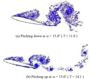
Unsteady Flow Past an Oscillating Airfoil
In order to examine the effectiveness of the present method, the two-dimensional unsteady separated flow past an oscillating NACA 0012 airfoil was computed by Etoh et al. (1997). Figure 3 shows
instantaneous flow patterns at the angle of attack D = 15.0oduring
pitching up and down motion, under condition of oscillation in pitch angle about the quarter chord point as D = 15.0o +5.0o sin : T at
Reynolds number Re=5.0 u 105, where T is the non-dimensional
time based on the cord length and the velocity of uniform flow, and
the non-dimensional time step was dT=0.026 and : was given as :
=1.0. It is clearly shown that in the case of pitching down motion, both a large dynamic stall vortex and a trailing edge vortex exist around the airfoil, whereas in the case of pitching up motion, the dynamic stall is in developing stage, and so the both vortices are not so large, yet.
(a) Pitching down at D = 15.0o ( T = 11.0 )
(b) Pitching up at D = 15.0o ( T = 14.1 )
Figure 3. Instantaneous flow patterns around an oscillating airfoil NACA
0012, here, D = 15.0o +5.0 o sin : T , Re = 5.0 u 105.
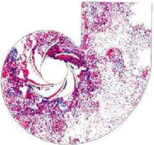
Unsteady Flow in a Centrifugal Pump
The advanced vortex method has been applied to such an engineering purpose as simulation of unsteady and complex flow through a two-dimensional centrifugal impeller by Zhu et al. (1998). Figure 4 shows an instantaneous pattern of flow through the impeller in the case of partial discharge (60% of the design flow
rate) at a non-dimensional time T=2.0 after the start of rotation at a
size was dT=0.01 and the non-dimensional value were based on the inlet meridian velocity at the design condition and the outer diameter of the impeller. It is clearly demonstrated that the flow becomes completely non-axi-symmetrical and some of blade-to-blade passages seem to be blocked with separation bubbles.
(a) Flow pattern represented by discrete vortices.
(b) Velocity vectors.
Figure 4. Two-dimensional unsteady flow in a centrifugal pump at 60% of the design flow rate.
Rotor-Stator Interaction in a Diffuser Pump
As the flow-unsteadiness generated by rotor-stator interaction in turbomachinery usually causes serious problems concerning vibration and noise, development of easy-to-handle methods have been expected to simulate the real unsteady-interaction without introducing either a sliding-surface between the rotating and stationary frames or turbulence models of time-mean type. In order to examine the applicability of the advanced vortex method for those purposes, the unsteady and interactive flows between a two-dimensional centrifugal impeller and a surrounding vaned diffuser were simulated by Zhu and Kamemoto (1999). In the calculation, each vane of the impeller and diffuser was represented 50 vortex panels, and the time step size and Reynolds number were taken as
dt=T/150 and Re=105 respectively, here T is the period of
revolution of impeller.
Figure 5 shows examples of calculated instantaneous pressure distribution at a time and periodic fluctuation of static pressure with time at a point close to the suction-side of leading edge of a diffuser vane compared with experimental data by Tsukamoto et al. (1995). It is found that there exist considerable differences of static pressure
in the flow field around the diffuser inlet corresponding to the relative position between impeller and diffuser vanes. And it is one of the most interesting points that the fluctuation of calculated
pressure coefficient Cp is in good agreement with experimental one
in its absolute value.
(a) Instantaneous pressure distribution
(b) Variation of static pressure with time at a point close to the suction-side of leading edge of a diffuser vane.
Figure 5. Interactive pressure distribution around rotor and stator vanes in a diffuser pump (100%).
Simulation of Forced Convective Heat Transfer Around a Circular Cylinder
Kamemoto and Miyasaka (1999) proposed a vortex and heat elements method and showed application results of analysis of unsteady and forced-convective heat transfer around a circular cylinder in a uniform flow. Figure 6 (a) and (b) respectively show an instantaneous temperature distribution in the flow field around a circular cylinder and the corresponding flow pattern at a
non-dimensional time T= 25.0 after the impulsive start of flow, where Re
= 104and Pr = 0.71. It is clarified that thermal crowds are formed
(a) Instantanenou temperature
(b) Instantaneous flow pattern
(
c) Time-averaged local Nusselt number distribution.Figure 6. Instantaneous temperature distribution and flow pattern. ( Re=104, Pr=0.71, Time=25.0 ).
Simulation of Three-Dimensional Unsteady Flows Through a Wind Turbine
In relation with further development of promising clean energy resources, investigations of unsteady and three-dimensional characteristics of flows around wind turbines are required. Especially, it is necessary to predict the features of complex vortical flows for design of suitable operational procedures under unexpected flow conditions. Corresponding to such requirements, simulation of three-dimensional and unsteady flows through the horizontal-axis wind turbine with a couple of blades of NACA0012 experimented by Vermeer (1991) was performed applying the advanced vortex method by Ojima and Kamemoto (2001). In the calculation, the blade was divided into 572 source and vortex panels (span wise: 22, sectional blade element: 26), and the time step size
and Reynolds number were taken as dtV/R=2ʌ/(200ȍ) and Re=VR/
Ȟ=1.0×10⁶, where V, R andȍ denote the blade tip velocity, the
rotational radius of the blade tip and angular velocity. Figure 7 (a) shows calculated instantaneous flow pattern represented by distribution of discrete vortex elements in operation at the tip speed
ratio Ȝ=V/U=7.5 after three times of rotor revolution, where U is a
wind velocity. At the initial stage of the flow, complex wake structure is formed behind the rotor blade due to interaction among starting vortices shed from the trailing edge and the longitudinal vortices shed from the tip and root of the blade. And it is observed that as time goes on, the starting vortices flow downstream and the longitudinal vortices tend to have dominant role in the flow field.
Figure 7 (b) shows comparison of calculated power coefficient Cpower and axial drag force coefficient CDaxis with experimental
results by Vermeer (1991). It is confirmed that both the power and the axial drag coefficients are reasonably coincident with experimental results.
(a) Instantaneous flow pattern behind a wind turbine after three times rotor revolution at tip speed ratioȜ=7.5
(b) Comparison of calculated wind turbine performance with experimental results.
Figure 7. Simulation of performance of a wind turbine.
Numerical Fish
lower is consisting of clockwise vortices. Figure 8 (b) shows the instantaneous pressure distribution on the skin of a trout obtained from 3-D calculation, here, the convex part shows a higher pressure region and the concave part is a lower pressure region. Figure 8 (c) shows the 3-D and complex vortex structures in the flow around the trout swimming at the best efficiency condition.
(a) Flow around a swimming trout (2-D) a trout (3-D).
(b) Instantaneous pressure distribution around
(c) 3-D vortex structures in the flow behind a trout
Figure 8. Flow around a numerical fish (trout).
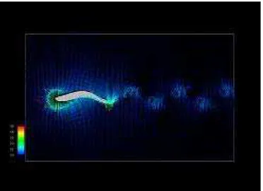
Pump-Turbine
In design and operation of a pump-turbine for hydroelectric power generation, it tends to become much more important to understand the effects of unsteady interaction among individual roles of stay vanes, guide vanes and rotating runner vanes on the unsteady characteristics of its operational performance. Making use of the advantage of the Lagrangian grid-free scheme of the present vortex method, interactive features of two-dimensional, unsteady and complex flows through a model pump-turbine were calculated, where the Reynolds number was Re = U2D2/Q = 6.0 u106, here U2
denotes peripheral velocity at the outlet diameter D2 of the runner
vanes. Figure 9 shows an instantaneous flow pattern in the whole passage during turbine-operation expressed by a number of velocity vectors. It was revealed that unsteady flow characteristics in the runner are essentially originated from the vortical flow features developed in the flow-passage through the stay vanes and guide vanes.
Figure 9. Instantaneous flow pattern in a pump-turbine during turbine-operation.
Mixed Flow Pump
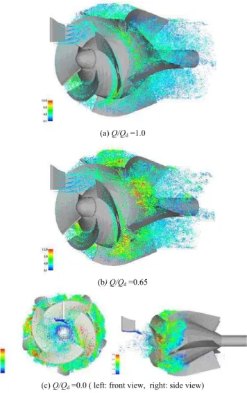
In order to predict the fluctuation of radial force acting on a rotating impeller, the internal flows of a mixed-flow pump were simulated by Kamemoto and Ojima (2004), for three operating conditions: the design point (Q/Qd=1.0 ) , an off-design point ( Q/Qd
= 0.65 ) and a shut-off point ( Q/Qd=0.0). This pump was
manufactured and tested by DMW Corporation in Japan, and it was composed of a 4 bladed mixed-flow impeller, 5 bladed guide vanes and an inlet whirl stop. Here, the outlet diameter of this impeller is 360 mm and the tip clearance is 0.4 mm. Specifications of the pump
are as follows: designed flow rate (Qd) =18.1 m
3
/min, head (H)
(a)Q/Qd =1.0
(b) Q/Qd =0.65
(c)Q/Qd =0.0 ( left: front view, right: side view)
Figure 10. Instantaneous flow patterns.
Figure 10 shows instantaneous flow patterns for the three operation conditions which are represented by a number of discrete vortex elements in the flow fields. It is observed that for both cases
of flow rate Q/Qd=1.0 and 0.65, any remarkable flow separations
are not detected around every impeller vane. In the case of Q/Qd
=0.65 shown in Fig.1 (b), however, strong tip-leakage vortices are formed from the tips of impeller vanes, and the tip-leakage vortices develop to the pressure side surface of the adjacent impeller vane or flow downstream in the passage of diffuser vanes. And then, a strong vortex bubble is formed in a vane-to-vane flow-passage in the diffuser. On the other hand, as shown in Fig.10 (c) in the case
of the shut-off operation (Q/Qd= 0.0), the reverse flow appears and
longitudinal vortices tend to develop in the inlet region of the pump. Figure 11 shows the computed radial fluid-forces acting on the
impeller under the three operation conditions. In this figure, Fx and
Fy denote the radial forces exerting on the impeller in the horizontal
directionx and the vertical direction y. It was confirmed that radial force components were periodically fluctuating with the interaction between rotating impeller-vanes and stationary guide-vanes, and the magnitude of fluctuations becomes larger as the flow rate decreases. Figure 12 shows the computed total head, shaft power, and pump efficiency in comparison with measured ones. Although only three cases of operation condition were simulated in the present study, the predicted characteristics of the pump reasonably agree with the experimental ones.
0 0.5 1 1.5 2 2.5 3 3.5
-400 -200 0 200 400
t/T0 Fx
, F
y
[N
]
: Fx
: Fy
(a) Q/Qd=1.0
0 0.5 1 1.5 2 2.5 3 3.5
-400 -200 0 200 400
t/T0 Fx
,
Fy
[N
]
: Fx
: Fy
(b) Q/Qd=0.65
Figure 11. Radial forces acting on the impeller.
0 0.5 1 1.5 2
-1500 -1000 -500 0 500 1000 1500
t/T0
Fx
, F
y
[ N
]
: Fx
: Fy
(c)Qd=0.0
Figure 11. Radial forces acting on the impeller.
0 10 20 30
0 5 10 15 20 25 30 35 40 45 50
0 20 40 60 80 100
Q [ m3/min ]
H
[
m
]
Ș
(%) ,
L
/2
(k
W
)
: H Exp : L Exp :Ș Exp : H Cal. (with WS) : L Cal. (with WS) :Ș Cal. (with WS) : H Cal. (without WS) : L Cal. (without WS)
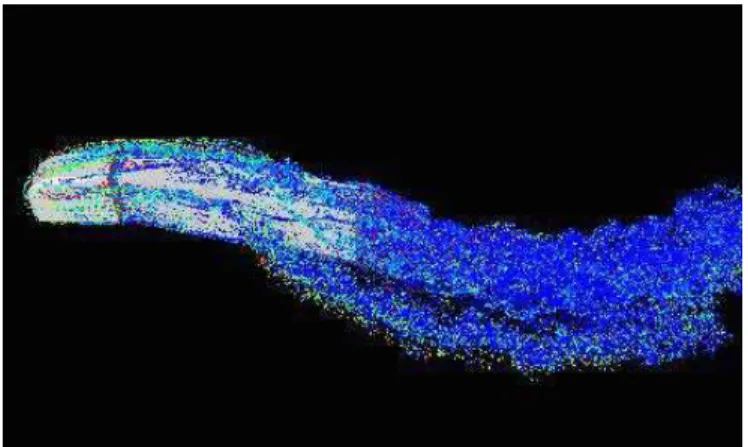
Pump Sump
In order to economize on cost and time in construction of a pump sump, application of numerical simulation technique has been expected to test whether undesirable suction vortices are detected around a suction opening of a pump or not, instead of experimental investigation using a scale model of the sump. Figure 13 shows an example of flow pattern in a pump sump of unsuitable configuration obtained from a trial calculation by the group of the present author. It is clearly observed that a submerged vortex is growing up under the suction opening.
Figure 13. Instantaneous flow pattern in a pump sump.
Tractor-Trailer
Recently, the group of the present author had an opportunity of presenting the result of our numerical investigation of aerodynamic features of a model of tractor-trailer at the United Engineering Foundation Conference on Aerodynamics of Heavy Vehicles, which was held in Monterey, 5-8 December, 2002. Figure14. shows an instantaneous flow patter around a tractor-trailer in condition of meandering motion, where Re = U0S1/2/Q = 3.0 u106 , S: is frontal area of the tractor. It was revealed from the calculation that considerable fluctuations of aerodynamic forces inevitably act on both the tractor and the trailer as a result of unsteady interaction of the flow separated from the tractor with the trailer
Figure 14. Instantaneous flow patter around a tractor-trailer in condition of meandering motion.
Conclusion
In this paper, mathematical background and numerical treatment of the advanced vortex method developed by the group of the present author were mainly explained, and several examples of
challenging application of the method were introduced. The discussion on attractive features and contribution of the advanced vortex method are summarized as follows:
(1) Since the present method is based on the Biot-Savart law, any grid generation is not necessary at all, for its time-splitting calculation of trajectory of discrete vortex elements in a flow field.
(2) Numerical calculation using the method is very stable because the main procedure is consisting of numerical integrations instead of finite difference calculations.
(3) The method is flexibly responsible to required accuracy of calculation, because the minimum scale of discrete vortex element can be determined according to resolution of vorticity distributions sufficient to represent the vortex structures to be solved.
(4) The method is available to direct numerical simulation of turbulent flow with introduction of small vortex elements of the Kolmogorov’s scale in the flow field.
(5) The method is useful for Lagrangian large eddy simulation with introduction of both vortex elements of rather large scale than the Kolmogorov’s scale and conventional Smagorinsky model.
(6) From the results of recent challenging works of application, it has been confirmed that the vortex method is available and useful for research in vortex dynamics and development in various engineering fields.
(7) It has been clear that the method consists of simple algorithm based on physics of flow and provides easy-to-handle and completely grid-free Lagrangian calculation of unsteady and vortical flows without use of any RANS type turbulence models.
Finally, it may be possible to consider that the advanced vortex method is one of the most capable methods to contribute to the new generation of computational fluid dynamics (CFD) and it yields a promising way toward virtual reality of unsteady and complex flows in vortex dynamics
Acknowledgements
The author would like to thank Dr. Takeda, Dr.Ido, and Dr. Yonayama of DMW Corporation in Japan for providing us with experimental data of the mixed-flow pump calculated in this study.
References
Chorin, A.J., 1973, “Numerical study of slightly viscous flow,” J. Fluid Mech. 57, pp.785-796.
Chorin, A.J., 1978, “Vortex sheet approximation of boundary layers,” J. Comp. Phys. 74, pp.283-317.
Cotte, G.H., Michaux, B., Ossia, S. and VanderLinden, G., 2002, “A comparison of spectral and vortex methods in three-dimensional incompressible flows,” J. Comp. Physics 175, pp.702-712.
Eldredge, J.D. Colonius, T. and Leonard, A., 2002, “A vortex particle method for two-dimensional compressible flow, “ J. Comp. Physics 179, pp.371-399.
Etoh, F., Kamemoto, K., Matsumoto, H. and Yokoi, Y., 1997, “Numerical simulation of flow around a rotary oscillating foil with constant amplitude angle by use of the vortex method,” Proc. 11th Symp. on CFD, Tokyo, pp.385-386.
Fisher, R.K., March, P.A., Mathur, D., Sotiropoulos, F. and Franke, G., 1998, “Innovative technologies brighten hydro’s future”, Proc. of the XIX IAHR Symposium on Hydraulic Machinery and Cavitation, Vol.1, pp.2-18.
Fukuda, K. and Kamemoto, K., 2004, “A Lagrangian redistribution model toward the construction of a turbulence model for vortex methods,” Trans. Japan Soc. Mech. Eng., B (in Japanese), (to be published).
Igarashi, T., 1984, “Flow and heat transfer in the separated region around a circular cylinder,” Trans. JSME. B 50-460, pp.3008-3014. (in Japanese).
Iso, Y., 2000, “Study on development of numerical fish,” Master Thesis at Department of Mechanical Engineering,, Yokohama National University.
Kamemoto K. and Miyasaka T., 1999, “Development of a vortex and heat elements method and its application to analysis of unsteady heat transfer around a circular cylinder in a uniform flow,” Proc. of 1st Int. Conf. on Vortex Methods, Kobe, Nov.4-5, pp.191-203.
Kamemoto, K. and Tsutahara, M., 2000, “VORTEX METHODS”, World Scientific..
Kamemoto, K. and Ojima, A., 2004, “Capability of the vortex method for virtual reality by computational hydraulics,” Proc. of 22nd IAHR Symp. on Hydraulic Machinery and Systems, Stockholm,June 29- July 2, Vol. B, B14-3.doc-1(11)-11(11).
Kiya M., Izawa S. and Ishikawa H., 1999, “Vortex method simulation of forced, impulsively started round jet,” Proc. of the 3rd ASME/JSME Joint Fluids Engng. Conf. San Francisco, July 18-22, FEDSM99-6813.
Leonard, A., 1980, “Vortex methods for flow simulations,” J. Comp. Phys. 37, pp. 289-335.
Leonard A. and Chua K., 1989, “Three-dimensional interaction of vortex tubes,” Pysica D (Nonlinear Phenomena), 37, pp.490-496.
Mansfield J.R., Knio O.M. and Meneveau C., 1998, “A dynamic LES scheme for the vorticity transport equation :Formulation and a priori tests,” J. of Comp. Phys., 145, pp.693-730.
Mansfield J.R., Knio O.M. and Meneveau C., 1999, “Dynamic LES of colliding vortex rings using a 3D vortex method,” J. of Comp. Phys., 152, pp.305-345.
Nakamura, H., Kamemoto, K. and Igarashi, T., 2001, “Analysis of unsteady heat transfer in the wake behind a circular cylinder in a uniform flow by a vortex and heat element method,” Proc. of 2nd Int. Conf. on Vortex Methods, Istanbul, Sept. 26-28, pp.235-242.
Nakanishi, Y. and Kamemoto, K., 1992, “Numerical simulation of flow around a sphere with vortex blobs,” J. Wind Engng and Ind. Aero., 46 and 47, pp.363-369.
Ojima A. and Kamemoto K., 2000, “Numerical simulation of unsteady flow around three dimensional bluff bodies by an advanced vortex method,” JSME Int. Journal, B, 43-2, pp.127-135.
Ojima, A. and Kamemoto, K., 2001, “Numerical simulation of unsteady flow through a horizontal axis wind turbine by a vortex method,” Proc. of 2nd Int. Conf. on Vortex Methods, Istanbul, Sept. 26-28, pp.173-180.
Pereira, L.A.A., Ricci, J.E.R., Hirata, M.H. and Neto, A.S., 2002, “Simulation of vortex flow about a circular cylinder with turbulence modeling,” Comp. Fluid Dynamics J., 11-3, pp.315-322.
Saltara F., Meneghini J.R., Siqueira C.R. and Bearman P.W., 1998, “The simulation of vortex shedding from an oscillating circular cylinder with turbulence modelling,” 1998 ASME FEDSM, Proc. of 1998 Conf. on Bluff Body Wakes and Vortex-Induced Vibration, Paper No. 13.
Sarpkaya, T., 1989, “Computational methods with vortices - the 1988 Freeman scholar lecture,” J. Fluids Engng., 111, pp.5-52.
Schmidt, E. and Wenner, K., 1941, “Warmeabgabe uber den Unfang eines angeblasenen geheizten Zylinders,” Forshg. Ing.-Wes. 12, pp.65-73.
Smith P.A. and Stansby, P.K., 1989, “An efficient surface algorithm for random-particle simulation of vorticity and heat transport,” J. Comp. Phys. 81, pp.349-371.
Tsukamoto H., Uno M., Hamafuku H. and Okamura T., 1995, “Pressure fluctuation downstream of a diffuser pump impeller,” Proc. of 2nd Joint ASME/JSME Fluid Engng. Conf., FED-vol. 216, pp.133.
Uhlman, J.S., 1992, “An integral equation formulation of the equation of motion of an incompressible fluid,” Naval Undersea Warfare Center T.R. 10-086.
Vermeer, N.J., 1991, “Performance measurements on a rotor model with Mie-vanes in the Delft open jet tunnel,” IW-91048R, Delft University
Winkelmans, G. and Leonard, A., 1988, “Improved vortex methods for three-dimensional flows,” Proc. Workshop on Mathematical Aspects of Vortex Dynamics. 25-35. Leeburg. Virginia.
Wu, J.C. and Thompson, J.E., 1973, “Numerical solutions of time-dependent incompressible Navier-Stokes Equations using an integro-differential formulation,” Computers & Fluids 1, pp.197-215.
Zhu, B., Kamemoto, K. and Matsumoto, H., 1998, “Computation of unsteady viscous flow through centrifugal impeller rotating in volute casing by direct vortex method,” Comp. Fluid Dynamics J. 7-3, pp.313-323.