Blind Identification of Underdetermined
Mixtures Based on the Characteristic Function:
The Complex Case
Xavier Luciani
, Associate Member, IEEE
, André L. F. de Almeida
, Member, IEEE
, and Pierre Comon
, Fellow, IEEE
Abstract—Blind identification of underdetermined mixtures can be addressed efficiently by using the second ChAracteristic Function (CAF) of the observations. Our contribution is twofold. First, we propose the use of a Levenberg-Marquardt algorithm, herein called LEMACAF, as an alternative to an Alternating Least Squares algorithm known as ALESCAF, which has been used recently in the case of real mixtures of real sources. Second, we extend the CAF approach to the case of complex sources for which the previous algorithms are not suitable. We show that the complex case involves an appropriate tensor stowage, which is linked to a particular tensor decomposition. An extension of the LEMACAF algorithm, called LEMACAF then proposed to blindly estimate the mixing matrix by exploiting this tensor decomposition. In our simulation results, we first provide perfor-mance comparisons between third- and fourth-order versions of ALESCAF and LEMACAF in various situations involving BPSK sources. Then, a performance study ofLEMACAF is carried out considering 4-QAM sources. These results show that the proposed algorithm provides satisfying estimations especially in the case of a large underdeterminacy level.
Index Terms—Blind identification (BI), blind source separation, characteristic function, complex sources, tensor decomposition, underdetermined mixtures.
I. INTRODUCTION
B
LIND Identification of linear mixtures (BI) has now become a major area of signal processing. For instance, since the theory of independent component analysis (ICA) [1], this subject has been at the center of many theoretical works while related methods and algorithms have been successfully used in applicative fields, notably in telecommunications [2], acoustic [3] or biomedical engineering [4], [5] among others; see [6], [7] for surveys.Manuscript received April 09, 2010; revised August 21, 2010; accepted Oc-tober 06, 2010. Date of publication OcOc-tober 25, 2010; date of current version January 12, 2011. The associate editor coordinating the review of this manu-script and approving it for publication was Dr. Philippe Ciblat.
X. Luciani is with the French Institute INSERM U642 and with the Univer-sity of Rennes 1, LTSI, 35042 Cedex, Rennes, France (e-mail: lucianix@gmail. com).
A. L. F. de Almeida is with Wireless Telecom Research Group, Department of Teleinformatics Engineering, Federal University of Ceará, 60455-760, Fort-aleza, Ceará, Brazil (e-mail: andre@gtel.ufc.br).
P. Comon is with the Laboratory Informatique Signaux et Systèmes de Sophia-Antipolis (I3S), UMR6070 CNRS-UNS, F06903 Sophia Antipolis cedex, France. He is also with INRIA, Galaad, F06902 Sophia Antipolis cedex, France (e-mail: pcomon@unice.fr).
Color versions of one or more of the figures in this paper are available online at http://ieeexplore.ieee.org.
Digital Object Identifier 10.1109/TSP.2010.2089625
In the meantime, tensor analysis has gained attention in nu-merous application areas involving data analysis such as psyco-metrics [8], arithmetic complexity [9], and chemopsyco-metrics [10], [11]. In particular, the Canonical Decomposition (CanD) [8] also known as PARAllel FACtor analysis (PARAFAC) [12] has met with success. One of the reasons is that CanD can often favorably replace Principal Component Analysis (PCA), when available data measurements can be arranged in a meaningful tensor form [13]. Indeed, the CanD comes with a nice unique-ness property [14]–[18] and some simple numerical algorithms [10], [19], [20].
Due to multiple connections between the two areas, these ad-vantages have been rapidly exploited for BI purposes [21]–[24]. In addition, tensor-based algorithms allow to solve the problem of underdetermined mixtures (i.e., when the number of sources is greater than the number of sensors), which arises in many practical situations, especially in telecommunications, and in which we are presently interested. A first class of algorithms exploits the trilinear nature of the observations, and the CanD of the data tensor provides a direct source estimation. For instance, this deterministic approach is widely used in fluores-cence spectroscopy [10], [11]. When the observation diversity is not sufficient, one can resort to a second class of algorithms, using the multilinearity properties of High-Order Statistics (HOS) [20]. A large majority of these algorithms involves a tensor containing the cumulants of the observations, the decom-position of which leads to the blind identification of the mixing matrix [23], [25]. This is notably the case of FOOBI [26], FOOBI2 [22] and 6-BIOME [27] algorithms, which use fourth-and sixth-order cumulant tensors, respectively. Nevertheless, a different class of BI methods not exploiting cumulants but the second ChAracteristic Function (CAF) of the observations, has been proposed in [28]–[30]. We are particularly interested in the approach originally proposed in [29], leading to efficient algorithms such as ALESCAF [30]. In that work, the authors showed that partial derivatives of the second characteristic function can be stored in a symmetric tensor, the CanD of which provides a direct estimation of the mixing matrix up to trivial scaling and permutation indeterminacies. In [30], the ALESCAF algorithm is applied to a data tensor constructed from third-order derivatives of the characteristic function. It is worth mentioning that the ALESCAF algorithm has only been applied to BI problems involving real sources (e.g., BPSK and 4-PAM). The present study notably generalizes the CAF approach to the case of complex mixtures of complex sources, which often occurs in digital communications and for which the ALESCAF algorithm needs non trivial extensions.
The paper is organized as follows. In Section II, the BI problem is formulated and the CAF approach is briefly pre-sented by first considering the case of real sources. A new LEMACAF algorithm that copes with the real case is also introduced in this section. In Section III, we transpose the CAF approach to the case of complex sources. A new core equation is obtained and an appropriate decomposition of the derivative tensor is detailed. In order to implement this more general approach, we propose a suitable algorithm called in Section IV. Computer simulation results considering both the real and complex cases are reported respectively in Sections V and VI. The paper is concluded in Section VII. Matlab codes including notably ALESCAF, LEMACAF and algorithms can be found at http://www.i3s.unice.fr/~pcomon/TensorPackage.html.
Notations: In the following, vectors, matrices and tensors are
denoted by lower case boldface , upper case boldface and upper case calligraphic letters, respectively. is the
coordinate of vector and is the column of matrix . The entry of matrix is denoted and the entry of the third-order tensor is denoted . Complex objects are underlined, their real and imaginary parts are denoted and , respectively. denotes the expected value of a random variable.
II. PROBLEMFORMULATION ANDCAF APPROACH IN THEREALCASE
We consider here the classical linear model of a noisy mix-ture of stationary sources received by an array of sensors. The mixture is instantaneous and underdetermined
and defined by a mixing matrix . Define also ,
and as the re-alizations of the observation, source and noise vectors, respec-tively, . According to this linear model we have
Algorithms from the CAF family use the partial derivatives of the observations characteristic function to identify the mixing matrix under the following assumptions:
. The mixing matrix does not contain pairwise col-inear columns.
. The sources are non-Gaussian and mutu-ally statisticmutu-ally independent.
. The number of sources is known.
It has been shown in former studies [31], [32] that is theoret-ically identifiable under these assumptions.
Here, we briefly recall the main steps of the CAF approach originally proposed in [29]. Let us denote and the second generating functions1of the observations and source ,
respectively
1In order to simplify notations and calculations, without any theoretical
impact, we prefer using the generating function instead of the characteristic function.
Replacing by its model and neglecting the noise contribu-tion leads to the decomposicontribu-tion of the observacontribu-tion generating function into the sum of the sources individual generating functions
Using the source independence property, we get
(1) Equation (1) is the core equation of the CAF approach in the real field. Differentiating (1) times with respect to compo-nents of , denoted , and defining
we obtain
(2) with and . These derivatives could be stored in a th-order tensor but in practice, the partial deriva-tives of are computed in points of . The objective is to increase the order of the tensor, aiming at achieving a better estimation quality. Hence, we now have a th-order data tensor, the last dimension describing the differentiation points. The key issue of the CAF approach is that (2) is nothing else but the rank- (truncated) CanD of the data tensor, which allows the identification of matrix . Indeed, when the number of sources is smaller than the generic rank of the tensor, this decomposition admits an essentially unique so-lution for and , (i.e., up to scaling and permutation of their columns), where is the matrix with entries .
The general structure of CAF algorithms can be summarized as follows:
1) Choose points of ;
2) Compute for each point order partial derivatives of and store the results in a tensor ;
3) Estimate from the rank- decomposition of . Note that the differentiation order is an input parameter of the algorithm. The higher the differentiation order, the higher the tensor order, and hence its generic rank for these dimen-sions. Consequently, increasing the differentiation order should allow to identify mixtures involving a larger number of sources without increasing the number of sensors. The price to pay is, of course, an increase in the algorithm complexity and probably a loss in robustness and accuracy.
estimation accuracy. In addition, the successful tensor-based ap-plications of the LM method in different apap-plications [19], [34], [35] has motivated us to introduce a LM-based algorithm called LEMACAF, which achieves the decomposition of higher-order tensors constructed from the derivatives of the characteristic function as follows: Define as the estimated matrix cor-responding to the mode of the CanD (2), , and as the estimated matrix corresponding to the -th mode. Let be the tensor built from the estimated matrices. Note that ideally we should have
and . We consider the mini-mization of the following quadratic cost function:
T (3)
where is the residue and is the parameter vector defined as
T T
T T T T T (4)
where maps a matrix or a tensor to a column vector by stacking its columns one below the other. The LM update at iteration is given by
(5) where denotes the Jacobian matrix given by:
, is the gradient vector given by , or equivalently: and is a positive regularization parameter. At every iteration , ,
, , and are updated. There are many ways to proceed, and we retained the scheme described in [36]:
1) Initialize and compute 2) Compute and deduce
3) Compute
were
is the second-order approx-imation of .
4) if then is accepted,
and . Otherwise is rejected, and .
Compact forms of the gradient vector and Jacobian matrix for a third-order tensor can be found in [34] and [20]. Those can be easily generalized for higher order tensors. After convergence, an estimate of the mixture is obtained from the average of
after a column-wise normalization.
It is worth mentioning that, although ELS refinements and symmetric constraints are applicable to improve the conver-gence speed of the LEMACAF algorithm, our preliminary numerical simulation study has shown no significant improve-ment. Therefore, these refinements are not considered here. Order 3 and 4 versions of the LEMACAF algorithm will be considered later in Section V.
III. EXTENSION TO THECOMPLEXFIELD
In this section, we generalize the BI problem based on the characteristic function to the complex field, i.e., to the case of complex mixtures of complex sources. Although the theoretical aspects are similar to the real case, (1) cannot be used directly in the complex field therefore the CanD of the derivatives given in (2) is no more valid in the complex sources case.
The generalization of the CAF approach to the complex case involves the following steps: i) choosing an appropriate core equation, ii) deduce the associated tensor decomposition by dif-ferentiating this core equation and, finally, iii) formulating an efficient algorithm to estimate the mixing matrix from the struc-ture of the obtained tensor decomposition. In this section we ad-dress the two first steps.
A. The New Core Equation
Observation and source vectors belong now to the com-plex field as well as the mixing matrix .
The second generating function of the observations, , can still be decomposed into a sum of marginal second generating functions of sources, , . In order to see this, start from the definitions of and in the complex field. Gen-erating functions of a complex variable are actually defined by assimilating to . Thus the second generating function of the source taken at the point of is defined as a function of the real and imaginary parts of
In a more compact form, we have
(6) This bijection also applies to . Hence, taken at the point
of is actually defined in by
where and and thus we have
Now, replacing by its model and neglecting the noise contri-bution yields
and (6) yields
Finally, we define two real matrices and so that . This leads to the new core equation that copes with the complex case
(7)
Note that defining and in and , respectively, in-stead of and allows their differentiation. Hence, the next step is the differentiation of (7).
B. Differentiation of
Let us define , and , so that belongs to . From these definitions, (7) can be rewritten as
(8) where
We also introduce three functions , and , respectively, defined by
and
Functions map to
This yields a compact representation of (8) as follows:
Now, we can compute the partial derivatives of
with respect to the real and imaginary parts of . Similarly to the real case, in order to have a sufficient diversity of equations, we have to use higher differentiating orders. The objective is to increase the order of the tensor, with the goal of achieving a better estimation quality. In the theoretical part of this study, we limit ourselves to second- and third-orders, being understood that equations
associated with higher differentiation orders can be obtained in a similar manner.
The number of equations can also be increased for a fixed differentiation order, by computing partial derivatives of in different points of , denoted here as ,
.
1) Order 2 Derivatives: At order 2, we obtain
(9)
(10)
(11)
where
Thereby, each of the three second-order derivatives (9)–(11) are given by a sum of four different third-order CanDs involving the elements of the mixing matrix in different ways. Note that, since all values of and are taken into consideration, (9)–(11) cover all the partial second-order derivatives. We show in Appendix A how to derive (9)–(11) from (8).
2) Order 3 Derivatives: By differentiating both (9) and (10)
with respect to and , , we can obtain the four different order 3 equations. Let us define
Using the fact that and , we get
(13)
(14)
(15) Thus, in the case of order 3 derivatives, each equation is now given by a sum of eight fourth-order CanDs involving the ele-ments of the mixing matrix in different ways.
C. Tensor Stowage and Decomposition
As we have seen in Section II, in the real case the second-order derivatives of can be stored in a third-order tensor, the CanD of which gives a direct estimation of the mixing matrix. The situation is quite different in the complex case but we still use a tensor approach to jointly exploit the different forms of derivatives. Let us first consider the case of second-order deriva-tives. From (9)–(11), we propose to build a fourth-order tensor
of dimensions containing all the three deriva-tive equations by concatenating all the associated decomposi-tions, as follows:
(16)
It appears that the CanD of these tensors or of any combination of those is insufficient here. Therefore CanD based algorithms such as ALESCAF are not pertinent in this case.
By applying the same reasoning to third-order (12)–(15), we can build a fifth-order tensor of dimensions
as
(17)
Our goal is to devise an algorithm capable of jointly esti-mating the real and imaginary parts and of the mixing matrix from or . This issue is addressed in the next section.
IV. ALGORITHM FOR THECOMPLEXCASE
A. Building the Derivative Tensor
First of all, we have to build or from realizations of and (16) or (17), respectively. Tensor entries are computed one by one just like in the real case. We call the first generating function of defined in by
(18) in order that . In practice, the expected value is estimated by the sample mean over all realizations. Note that this estimator is consistent but it leads to a biased estimation of the partial derivatives of , if the latter are computed by finite differences of (18). As in [30], it is preferred to compute formal derivatives, and estimate the obtained expressions with the help of sample means.
Let us define as the partial derivatives of
The first-order derivatives of are given by
(19)
At order 2, the elements of (i.e., second-order derivatives) are obtained by differentiating (19)
(20)
(21)
(22)
At order 3, the elements of (i.e., third-order derivatives) are obtained by differentiating order 2 equations
(23)
(24)
(25)
(26)
B. Description of the Algorithm
The proposed algorithm is named , where “O” indicates the order of differentiation. For instance
consists of iteratively fitting the tensor built from model (9)–(11) to built from (20)–(22), using the Levenberg-Marquardt method.
The basic scheme of is thus similar to the LEMECAF one. However, in this case, we are dealing with highly structured fourth- and fifth-order tensors (when con-sidering and , respectively). Thereby the parameter vector, the cost function and the construction of the Jacobian matrix and the gradient vector used at each LM update are completely different, involving more complicated calculations. In the case, the quadratic cost function is defined as:
T
where is the residue and is the parameter vector
T T T T T T
T T T T T
The LM update at iteration is still given by
where and denotes the Jacobian matrix and gradient vec-tors respectively. These are obtained by computing analytically
and .
Elements of the Jacobian matrix are given in Appendix B for and . At every iteration , , , , and are updated according to the LEMACAF scheme, described in Section II. After convergence of the algorithm, an estimate of the mixture is obtained by
(up to column permutation and scaling).
V. SIMULATIONRESULTSPARTI: THEREALCASE
In this section, we compare both ALESCAF and LEMACAF algorithms on mixtures of synthesized BPSK sources, with the well-known 6-Blind Identification of Overcomplete MixturEs (BIOME) algorithm [27], also referred to as Blind Identi-fication of mixtures of sources using Redundancies in the daTa Hexacovariance matrix (“BIRTH”) when the chosen cumulant order is 6. For these comparisons, we retained third-and fourth-order versions of ALESCAF third-and LEMACAF (re-spectively, ALESCAF-3, ALESCAF-4, LEMACAF-3, and LEMACAF-4). Note that as far as we know, ALESCAF-4 had never been implemented before. Algorithms are evaluated according to the normalized mean square estimation error (NMSE)
TABLE I
REALCASE, MINIMAL, MAXIMAL ANDMEDIANVALUE OF THENMSE ACCORDING TO THENUMBER OFSOURCESCOMPUTEDFROM100 MONTECARLORUNS
Fig. 1. Real case, NMSE distribution according to the number of sources.
NMSE values are computed from 100 independent realizations of source and mixing matrices. The number of sensors, , is always equal to 3. Concerning the CAF algorithms, the derivatives are computed at 8 different points (that is, ), randomly drawn in the range .
A. Impact of the Number of Sources
In this first simulation the noise is null, we use 10 000 ob-servations and we made three Monte Carlo experiments corre-sponding to three different source numbers ( , , ). Histograms of the identification error are represented in Fig. 1, for the five algorithms, and summarized in Table I.
a) 4 sources: Whatever the algorithm most NMSE values
range between and and the largest part is between and , indicating that all algorithms perform well. There is no significant difference between CAF algorithms which all performed slightly better than 6-BIOME.
b) 5 sources: All NMSE values are greater than .
ALESCAF-4 and LEMACAF-4 provide the best results
(40% of NMSE values are less than ) followed by the order three CAF algorithms (30%) and lastly 6-BIOME (less 20%). According to the median error values, LEMACAF seems more efficient than ALESCAF.
c) 6 sources: A majority of Monte Carlo runs did not
con-verge. This holds true for all algorithms. Only the CAF algorithms provide some (less than 10%) NMSE values under . In this case, with about 45% of NMSE values under , order 4 algorithms are clearly better than order 3 (15%). 6-BIOME is on the average with more than 30%. Once again LEMACAF is slightly better than ALESCAF.
d) Conclusion: In this first experiment, it clearly appears that
order 4 algorithms are particularly attractive when the un-derdeterminacy level is high, at the opposite of order 3 algorithms, while 6-BIOME has average results. It also appears that LEMACAF usually provides a better conver-gence than ALESCAF.
B. Impact of the Number of Observations
Now, the number of sources is set to 4, and the number of observations is varied from 200 to 10 000. The results are shown in Fig. 2 in the form of histograms. The variation of the median value of the NMSE is plotted in Fig. 3.
As expected, the performance improves linearly with an increase in the number of observations. Globally, beyond 5000 observations the majority of NMSE values are lower than . Between 5000 and 1000 observations the NMSE values are comprised between and . We have observed no significant differences among the performance of the four CAF algorithms. On the other hand, according to the median plot of Fig. 2, they all give better results than 6-BIOME in all the eight situations. Additionally, these results also show that the difference between the two classes of algorithms is more significant under 700 observations.
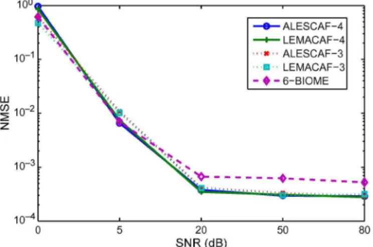
C. Impact of the Signal to Noise Ratio
Finally, the algorithms are compared with the help of six Monte Carlo experiments corresponding to different SNRs, and considering 4 sources and 10 000 observations. The results are presented in Fig. 4 in an histogram form, while the evolution of the median NMSE value is plotted on Fig. 5.
Fig. 2. Real case, NMSE distribution according to the number of observations.
Fig. 3. Real case, evolution of the NMSE median value according to the num-bers of observations.
0 dB SNR. Note that, in this case, very few Monte Carlo re-sults are satisfactory whatever the algorithm. In the middle of the SNRs range (i.e., around 5 dB), LEMACAF4, ALESCAF4 and
6-BIOME present similar performances. Finally, LEMACAF is once again slightly better than ALESCAF.
D. Discussion
From the previous simulation results, it can be concluded that the CAF algorithms perform similarly in more “favorable” sce-narios (i.e., when the SNR and the number of observations are high and the undeterminacy level is low). However a clear dis-tinction between third- and fourth-order algorithms can be made in more difficult cases. As expected, the improvement obtained with higher order algorithms becomes significant when the inde-terminacy level increases. These results show that LEMACAF is an interesting alternative to ALESCAF. It is worth mentioning that LEMACAF converges faster than ALESCAF at the price of a higher computational complexity per iteration [20]. Al-though ALESCAF can still be useful with larger tensors, we think that LEMACAF should be recommended in more prac-tical situations.
Fig. 4. Real case, NMSE distribution according to the SNR.
Fig. 5. Real case, Evolution of the median NMSE value according to the SNR.
algorithm, especially when the number of observations is low and/or when the underdeterminacy level is high and/or when the SNR is above 5 dB. Indeed, in many situations, the 6-BIOME
algorithm offers similar performance as third-order CAF algo-rithms however it is consistently overpass by fourth-order CAF algorithm.
VI. SIMULATIONRESULTSPARTII: THECOMPLEXCASE
TABLE II
COMPLEX CASE, MINIMAL, MAXIMAL ANDMEDIANVALUE OF THENMSE ACCORDING TO THE
NUMBER OFSOURCES, COMPUTEDFROMSEVERALMONTECARLORUNS
Fig. 6. Complex case, NMSE distribution according to the number of sources.
A. Impact of the Number of Sources
We have made three different experiments corresponding to 4, 5, and 6 sources. The SNR is set to 20 dB. An histogram of the NMSE values is given in Fig. 6. Minimal, maximal and median value of the NMSE according to the number of source are given in Table II.
e) 4 sources: Fig. 6 clearly shows that both
algorithms provide statistically the best estimations, since about 40% of the obtained NMSE values are under against about only 16% for 6-BIOME. Note also that performs better than
: 18% of its NMSE values are under against 8% for besides only 8% are above against 14% for
(and 20% for 6-BIOME). Table II confirms this ob-servation. Note that the maximum value obtained with
is only 0.01.
f) 5 sources: For the three algorithms, there are very few
values under whereas a significant number of NMSE values are between and .
dominates with 50% of its NMSE values in this range, against 40% for the other algorithms. More generally, in this case, and 6-BIOME are slightly equivalent. This is confirmed by the median values stored in Table II.
g) 6 sources: 15 Monte Carlo runs have been used for
this test. This is a difficult situation where the under-determinacy level is high. Note that the NMSE values of 6-BIOME do not decrease under , contrary to and . In addition 6-BIOME provides only one values under against 3 for and 6 for . However, according to the median values, the 6-BIOME algorithm offers a performance that is in between third-and fourth-order CAF algorithms.
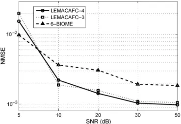
B. Impact of the Signal to Noise Ratio
In the following simulations, the algorithms are compared for five SNR values (5, 10, 20, 30, and 50 dB), and assuming 4 sources. The results are depicted in Fig. 7 and 8. Regarding the median NMSE plotted in Fig. 8, it can be observed that perfor-mances logically degrade as the SNR decreases. However, one can clearly discriminate two opposite situations. Above 5 dB SNR, and offer similar performances and clearly outperform the 6-BIOME algorithm. On the other hand, at around 5 dB SNR, 6-BIOME provides better results.
The histograms plotted in Fig. 7 refine these observations. In the SNR range from 50 to 10 dB, the number of NMSE values above remains stable while a large majority of NMSE values is consistently located between and . This means that all algorithms perform satisfactorily in these conditions.
Fig. 7. Complex case, distribution according to the SNR.
Fig. 8. Complex case, evolution of the NMSE median value according to the SNR.
and respectively. In other words, it confirms our previous observations, since for SNR
values which are higher than 5 dB, CAF algorithms are more attractive than 6-BIOME, otherwise the latter is slightly more efficient. Furthermore, it is worth noting that at the exception of the 10 dB SNR case, consistently provides a larger number of NMSE values located under than does. Therefore, higher order version of still promises a better convergence (from a statistical point view).
VII. CONCLUSION
In this paper we have proposed several new contributions to the blind identification of undertermined mixtures using the characteristic function. Notably, we have extended the theory of CAF approach to the case of complex mixtures of complex sources. Hence an appropriate core equation was developped to cope with the complex case. By differentiating this core equation, we obtained a generalized tensor decom-position from which an estimation of the mixing matrix can be deduced. A Levenberg-Marquardt algorithm, herein called , was proposed to blindly estimate the mixing matrix by exploiting the structure of this tensor decomposition. Two performance studies were carried out. In a first part, a new LEMACAF algorithm, suitable for the real case, was compared to higher order versions of ALESCAF in various situations involving BPSK sources. In a second part, the performance of the algorithm using third- and fourth-order derivatives were evaluated from mixtures of 4-QAM sources. In each situation, the 6-BIOME algorithm was used as a reference for the comparison.
From our simulation results, in both the real and complex cases, we can recommend the use of the CAF family of algo-rithms, especially in the case of highly underdetermined mix-tures and the medium-to-high signal to noise ratios (say, above 5 dB). The choice of the differentiation order is led by the de-sired tradeoff between estimation accuracy and computational cost. In the least favorable situation, we recommend the use of higher order derivatives. In practice it appears that order 3 ver-sions are enough to compete with (and often outperform) an al-gorithm using 6-order statistics such as 6-BIOME.
In the case of real sources, although is appli-cable, one should prefer ALESCAF or LEMACAF algorithms since they are less computationally costly. Since both offer quite similar performance in terms of estimation error, the choice is led by the convergence speed, which means that ALESCAF is only preferable for large tensors.
Finally, as we have pointed out previously, the higher-order derivative tensors that arise when working with complex mix-tures of complex sources follow a decomposition in a sum of structured CanD blocks. We think that block decompositions [37] can be used to decompose these tensors. In this context, it would be interesting to study uniqueness issues and their prac-tical implications to the CAF-based BI problem.
APPENDIXA
COMPUTATIONALDETAILS OFFIRST-ANDSECOND-ORDER
DERIVATIVES OF
The differentiation of (8) with respect to , gives
(27) In the same way, the differentiation with respect to gives
(28)
Now we differentiate (27) and (28) with respect to and , .
(29) Substituting (27) into (29) yields
(30)
Finally, using the fact that , we obtain (9). The same reasoning can be applied to obtain the successive derivatives of (28) and (27) with respect to and , hence (10) and (11).
APPENDIXB
JACOBIANFORMULATION FOR AND
We provide the details of the structure of the Jacobian matrix used in and , (higher orders
can be obtained in a similar manner). Although the Jacobian can be computed automatically for a given differentiation order, this solution is usually very time consuming. Therefore, one would rather use the following precalculated entries. The gradient can be directly deduced from the Jacobian and the error term.
A. Jacobian for
is the multiway error function which is defined as follows:
The Jacobian matrix of is built as a blocks matrix
, , , , contain partial derivatives of with respects to the elements of , , , , and , re-spectively. For instance, defining
and
with , , , , and we have
B. Jacobian for
At order 3, we have now a blocks matrix
and we define
with , , , ,
, and Block entries are computed by differentiation of [(12)–(15)].
REFERENCES
[1] P. Comon, “Independent component analysis,” inHigher Order Sta-tistics, J.-L. Lacoume, Ed. Amsterdam, London: Elsevier, 1992, pp. 29–38.
[2] C. Estevao, R. Fernandes, G. Favier, and J. C. Mota, “Blind channel identification algorithms based on the PARAFAC decomposition of cu-mulant tensors: The single and multiuser cases,”Signal Process., vol. 88, no. 6, pp. 1382–1401, 2008.
[3] F. Asano, S. Ikeda, M. Ogawa, H. Asoh, and N. Kitawaki, “Com-bined approach of array processing and independent component anal-ysis for blind separation of acoustic signals,”IEEE Trans. Speech Audio Process., vol. 11, no. 3, pp. 204–215, 2003.
[4] A. Kachenoura, L. Albera, L. Senhadji, and P. Comon, “ICA: A poten-tial tool for BCI systems,”IEEE Signal Process. Mag. Special Issue on Brain-Comput. Interfaces, vol. 25, no. 3, pp. 57–68, 2008.
[5] L. de Lathauwer, D. Callaerts, B. de Moor, and J. Vandewalle, “Fetal electrocardiogram extraction by source subspace separation,” inProc. IEEE Workshop on Higher Order Statistics, Girona, Spain, 1995, pp. 134–138.
[6] A. Cichocki and S.-I. Amari, Adaptive Blind Signal and Image Pro-cessing. New York: Wiley, 2002.
[8] J. D. Carroll and J. J. Chang, “Analysis of individual differences in multidimensional scaling via n-way generalization of Eckart-Young decomposition,”Psychometrika, vol. 35, no. 3, pp. 283–319, 1970. [9] P. Bürgisser, M. Clausen, and M. A. Shokrollahi, Algebraic Complexity
Theory. New York: Springer, 1997, vol. 315.
[10] R. Bro, “PARAFAC, tutorial and applications,”Chemom. Intel. Lab. Syst., vol. 38, pp. 149–171, 1997.
[11] C. A. Stedmon, S. Markager, and R. Bro, “Tracing dissolved organic matter in aquatic environments using a new approach to fluorescence spectroscopy,”Marine Chem., vol. 82, no. 3–4, pp. 239–254, 2003. [12] R. A. Harshman, “Foundations of the Parafac procedure: Models and
conditions for an explanatory multimodal factor analysis,” UCLA Working Papers in Phonet., vol. 16, pp. 1–84, 1970.
[13] A. Smilde, R. Bro, and P. Geladi, Multi-Way Analysis. New York: Wiley, 2004.
[14] R. A. Harshman, “Determination and proof of minimum uniqueness conditions for PARAFAC-1,”UCLA Working Papers in Phonet., vol. 22, pp. 111–117, 1972.
[15] J. B. Kruskal, “Three-way arrays: Rank and uniqueness of trilinear de-compositions,”Linear Algebra and Appl., vol. 18, pp. 95–138, 1977. [16] J. M. F. Ten Berge and N. D. Sidiropoulos, “On uniqueness in
CAN-DECOMP/PARAFAC,”Psychometrika, vol. 67, pp. 399–409, 2002. [17] T. Jiang and N. D. Sidiropoulos, “Kruskal’s permutation lemma and the
identification of CANDECOMP/PARAFAC and bilinear models with constant modulus constraints,”Trans. on Signal Process., vol. 52, no. 9, pp. 2625–2636, 2004.
[18] L. de Lathauwer, “A link between canonical decomposition in multi-linear algebra and simultaneous matrix diagonalization,”SIAM J. Ma-trix Anal., vol. 28, no. 3, pp. 642–666, 2006.
[19] G. Tomasi and R. Bro, “A comparison of algorithms for fitting the parafac model,”Comput. Stat. Data Anal., vol. 50, pp. 1700–1734, 2006.
[20] P. Comon, X. Luciani, and A. L. F. de Almeida, “Tensor decomposi-tions, alternating least squares and other tales,”J. Chemometr., vol. 23, no. 9, pp. 393–405, Sept. 2009.
[21] N. D. Sidiropoulos, G. B. Giannakis, and R. Bro, “Blind PARAFAC receivers for DS-CDMA systems,”Trans. Signal Process., vol. 48, no. 3, pp. 810–823, 2000.
[22] L. de Lathauwer and J. Castaing, “Blind identification of underdeter-mined mixtures by simultaneous matrix diagonalization,”IEEE Trans. Signal Process., vol. 56, no. 3, pp. 1096–1105, Mar. 2008.
[23] P. Comon, “Blind identification and source separation in 223 under-determined mixtures,”IEEE Trans. Signal Process., pp. 11–22, Jan. 2004.
[24] A. L. F. de Almeida, G. Favier, and J. C. M. Mota, “PARAFAC-based unified tensor modeling for wireless communication systems with ap-plication to blind multiuser equalization,”Signal Process., vol. 87, no. 2, pp. 337–351, 2007.
[25] J. F. Cardoso, “Super-symmetric decomposition of the fourth-order cu-mulant tensor. Blind identification of more sources than sensors,” in
Proc. ICASSP’91, Toronto, Canada, 1991, pp. 3109–3112.
[26] L. de Lathauwer, J. Castaing, and J-. F. Cardoso, “Fourth-order cu-mulant-based blind identification of underdetermined mixtures,”IEEE Trans. Signal Process., vol. 55, no. 2, pp. 2965–2973, Feb. 2007. [27] L. Albera, A. Ferreol, P. Comon, and P. Chevalier, “Blind identification
of overcomplete mixtures of sources (BIOME),”Lin. Algebra Appl., vol. 391, pp. 1–30, Nov. 2004.
[28] A. TALEB, “An algorithm for the blind identification ofnidependent signals with 2 sensors,” inISSPA’01, Kuala Lumpur, 2001, vol. 1, pp. 5–8.
[29] P. Comon and M. Rajih, “Blind identification of complex underdeter-mined mixtures,” inICA Conf., Granada, 2004, pp. 105–112. [30] P. Comon and M. Rajih, “Blind identification of under-determined
mixtures based on the characteristic function,”Signal Process., vol. 86, no. 9, pp. 2271–2281, 2006.
[31] A. M. Kagan, Y. V. Linnika, and C. R. Rao, “Characterization prob-lems in mathematical statistics,” inProbability and Mathematical Sta-tistics. New York: Wiley, 1973.
[32] W. Feller, An Introduction to Probability Theory and its Applica-tions. New York: Wiley, 1966, vol. II.
[33] M. Rajih, P. Comon, and R. Harshman, “Enhanced line search: A novel method to accelerate PARAFAC,”SIAM J. Matrix Anal. Appl., vol. 30, no. 3, pp. 1148–1171, Sep. 2008.
[34] D. Nion, “Methodes PARAFAC generalisees pour l’extraction aveugle de sources. Application aux systemes DS-CDMA,” Thesis, Univ. Cergy-Pontoise, Cergy-Pontoise, 2007.
[35] A. L. F. de Almeida, X. Luciani, and P. Comon, “Blind identification of underdetermined mixtures based on the hexacovariance and higher-order cyclostationarity,” inProc. SSP’09, Cardiff, 2009, pp. 669–672.
[36] K. Madsen, H. B. Nielsen, and O. Tingleff, “Methods for non-linear least squares problems,”Tech. Univ. Denmark, Informat. and Math. Model., vol. 2.
[37] L. de Lathauwer, “Decompositions of a higher-order tensor in block terms-part II: Definitions and uniqueness,”SIAM J. Matrix Anal. Appl., vol. 30, no. 3, pp. 1033–1066, Sep. 2008.
Xavier Luciani(A’09) was born in Toulon, France, in 1979. In 2003, he received both the ISEN engi-neering diploma (College of Electronic and Numeric Engineering) and the Master’s degree in signal pro-cessing from the University of Toulon, France, and the Ph.D. degree in engineering sciences from the University of Toulon in 2007.
From March 2008 to September 2009, he held a postdoctoral position with the I3S Laboratory, Sophia Antipolis, France. He is currently a Postdoctoral Re-searcher with the LTSI Laboratory, U642, INSERM and the University of Rennes 1, France. Its research interests have been in tensor modeling of fluorescence signals, blind source separation and blind identifica-tion based on tensor approaches, algorithms for joint diagonalizaidentifica-tion and tensor analysis, and applications to chemometrics and telecommunications.
André L. F. de Almeida(M’08) received the B.Sc. and M.Sc. degrees in electrical engineering from the Federal University of Ceará, Brazil, in 2001 and 2003, respectively, and the double Ph.D. degree in sciences and teleinformatics engineering from the University of Nice, Sophia Antipolis, France, and the Federal University of Ceará, Fortaleza, Brazil, in 2007.
In 2002, he was a Visiting Researcher with Ericsson Research, Stockholm, Sweden. He was a Postdoctoral Fellow with the I3S Laboratory, CNRS, Sophia Antipolis, from January to December 2008. He is currently an Assistant Professor with the Department of Teleinformatics Engineering of the Federal University of Ceará, Fortaleza. He is also a Senior Researcher with the Wireless Telecom Research Group (GTEL), where he has worked on several funded research projects. His research interests lie in the area of signal processing for communications, including blind identification and signal separation, space-time processing, multiple-antenna techniques, and multicarrier communications. His recent work has focused on the development of tensor models for transceiver design in wireless communication systems.
Pierre Comon(M’87-SM’95-F’07) received the de-gree in 1982, and received the Doctorate dede-gree in 1985, both from the University of Grenoble, France. He received the Habilitation to Lead Researches in 1995 from the University of Nice, France.
He has been in industry for 13 years, first with Crouzet-Sextant, Valence, France, between 1982 and 1985, and then with Thomson Marconi, Sophia-An-tipolis, France, between 1988 and 1997. He spent 1987 with the ISL Laboratory, Stanford University, CA. He joined the Eurecom Institute, Sophia-An-tipolis, in 1997 and left during fall 1998. He is now Research Director with CNRS, where he has been since 1998, also at the Laboratory I3S, Sophia-An-tipolis. His research interests include high-order statistics (HOS), blind deconvolution and equalization, statistical signal and array processing, tensor decompositions, multiway factor analysis and its applications to biomedical end environment.
Dr. Comon was an Associate Editor of the IEEE TRANSACTIONS ONSIGNAL