Credit Bubbles and Misallocation
Pierluca Pannella
⇤†August 11, 2017
Please, download updated version from here
Abstract
Why are bubbles harmful to the economy? According to a recent literature on rational bubbles, the problem is the burst that causes a misallocation of funds and triggers a recession. This paper proposes a theory of rational bubbles where the boom, not the ensuing bust, reduces the output by promoting a misallocation of factors. As in recent literature, financial markets are imperfect and the rise of a bubble alleviates credit constraints and boosts capital accumulation. However, capital accumulation occurs in unproductive sectors and aggregate output is reduced. The result is driven by the fact that heterogeneous borrowers have an advantage with respect to issuing different types of debt contracts. In normal times, High-productive borrowers have higher collateral and thereby attract most of the funds. In bubbly times, borrowers can also issue “bubbly debt,” a debt that is repaid with future debt. The possibility to keep a pyramid scheme and raise bubbly debt depends on the probability of surviving in the market. Therefore, a bubble misallocates resources towards borrowers with low fundamental risk, even if they invest in projects with lower productivity. An augmented version of the model with nominal rigidities is proposed to explain the timing of expansions and recessions during “bubbly episodes”: the initial boom in output is caused by a positive demand effect; the long run reduction in TFP is driven by a misallocation process. The theory is supported by evidence on between-industry misallocation in the years preceding the 2008 financial crisis.
JEL classification: E32, E44, O16
Keywords: bubbles, credit, misallocation, financial frictions, productivity
⇤PhD Candidate, Vancouver School of Economics, The University of British Columbia.
†I wish to thank Paul Beaudry and Viktoria Hnatkovska for their guidance and advice. I would also like to thank Amartya
1 Introduction
In recent decades modern economies have experienced large fluctuations in aggregate credit. Periods of high growth have typically been followed by periods of decline or sudden busts. What drives these cycles is a current subject of research and no consensus has yet been reached. A growing literature links these periods of extraordinary credit growth to the emergence of a bubble. In particular, recent papers on rational bubbles point to the role of asset bubbles in easing the transfer of funds when credit is constrained. According to these sources, bubbles boost the productive efficiency of the economy by improving the allocation of financing - the burst of the bubble initiates a recession. However, there exists an alternative view proposing that credit booms and bubbles actually induce a direct misallocation of resources in the economy.
This paper contributes to the debate in two ways. First, it provides evidence that favors the misallocation view by analyzing the between-industry allocation of factors across Western countries in the years prior to the 2008 financial crisis. Second, it builds on recent theories put forward in the literature on rational bubbles to support this alternative hypothesis. I propose that it is the emergence of a bubble that reduces the output by promoting a misallocation of resources.
The original theory of rational bubbles was introduced by Tirole (1985). In Tirole’s framework, a bubble, defined as an asset with a zero market fundamental, can appear when the economy is dynamically ineffi-cient; i.e., when the marginal return on capital is smaller than the growth rate of the economy. Bubbles, then, enhance the inter-temporal allocation of resources and reduce the stock of capital. However, dynamic inefficiency was considered empirically irrelevant by most economists at the time.1 In addition, real bubbly
episodes are typically characterized by a boom in capital accumulation, a phenomenon that is counterfactual to the capital crowding-out predicted by the model. Recent papers relax the condition for the existence of rational bubbles and relate the arrival and burst of a bubble to credit dynamics. In fact, market returns can be lower than the growth rate even if the economy is dynamically efficient once we allow for imperfections in financial markets.2 According to Kocherlakota (2009), Martin and Ventura (2012, 2016), and Miao and
Wang (2012) a bubble improves the intra-temporal allocation of funds, from unproductive agents to credit-constrained productive ones.3 Intuitively, a bubble in the asset market raises the value of collateral, relaxes
the borrowing constraint, and therefore increases the amount of credit in the economy.4 In these models the
positive reallocation of investment supports a crowding-in of capital.
1See Abel, Mankiw, Summers and Zeckhauser (1989) and Geerolf (2013) for an empirical investigation on dynamic inefficiency. 2Woodford (1990) had already shown that financial frictions could relax the conditions for rational bubbles.
3Kocherlakota (2009) and Miao and Wang (2012) present models with infinite lived agents facing productivity shocks. Martin
and Ventura (2012, 2016) rely on an Over-Lapping Generations model with generations of productive and unproductive agents.
4In Kocherlakota (2009), Miao and Wang (2012) and Martin and Ventura (2016) the bubble is on the assets playing the role
of collateral. The main specification in Martin and Ventura (2012) has no explicit collateral constraint but the model can be reinterpreted with this constraint.
These recent papers on rational bubbles can replicate aggregate macroeconomic facts, such as the rise in investment rate during a credit boom and the start of a recession at the bust. Nonetheless, I question the reallocation channel which drives their result. My theory suggests that a bubble still alleviates credit constraints and raises the stock of capital. However, this is in favor of low productivity sectors.5
In Section 2, I provide the evidence that motivates my model. I investigate the relationship between credit growth and factor allocation in the years preceding the 2008 financial crisis. Specifically, I compare the change in between-industry allocation for a sample of Western countries that experienced a differential growth in credit. The result is that larger credit booms favored the expansion of industries with low Total Factor Productivity growth. In particular, companies from less productive industries relatively increased their leverage in the countries with a higher credit growth. In the following sections I place these facts inside the rational bubble framework.6
The theoretical contribution of the paper is presented in two steps, described in Sections 3 and 4. First, in a stylized model I derive the necessary conditions for bubbles inducing a misallocation of factors. Second, in a richer model I introduce a motivation for bubbles appearing and boosting capital accumulation in low productivity sectors.
My setup is based on the classical Over-Lapping Generations framework. In the model there are two types of agents: workers and investors. Workers earn their wage when young but have no technology to store their income for consumption when old. Investors, on the other hand, can invest today in order to obtain working capital tomorrow. A borrowing constraint limits the credit between workers and investors. However, the latter can potentially expand the funds they raise by issuing bubbly debt, a debt that will not be repaid with future income but with the purchase of this debt by a new generation of workers. It is worth noting that the emergence of bubbly debt is subject to workers’ beliefs regarding future repayment.
A main feature in the model is heterogeneity in investor productivity. In Section 3, agents’ beliefs will not only determine the rise of bubbly debt but also the identity of the issuers. Notably, the ability to issue bubbly debt does not depend on the productivity of an investor, since he will not be responsible for repayment. If workers buy bubbly debt issued by low productive investors, the outcome is a misallocation of resources away from more productive investors.
The mechanism described in Section 3 illustrates how a credit bubble can drag the economy into an
5To my knowledge, factor misallocation in a rational bubble environment has only been discussed in Miao and Wang (2014).
According to them a bubble can arise in a specific sector. However, a sector-specific bubble does not produce any direct misallocation. In keeping with the rest of the literature, the bubble still increases the productive efficiency of the sector. The overall productivity of the economy is negatively affected because the specific sector produces a negative externality on the rest of the economy.
6There are alternative theories that link credit booms and misallocation. For example Cecchetti and Kharroubi (2015) show
that an expansion of the financial sector misallocates high-skilled workers from more productive sectors. Alternatively, Gopinath, Kalemli-Ozcan, Karabarbounis and Villegas-Sanchez (2015) describe an environment in which larger firms have an advantage in accessing credit.
inefficient allocation of factors. There are, however, two drawbacks to this model. First, it does not say anything about how the borrowers issuing bubbly debt are selected. Second, it predicts a reduction in aggregate capital when factors are misallocated. This prediction is counterfactual to the large accumulation of capital that preceded the 2008 financial crisis.
In Section 4, I address both issues by making a substantial addition to my model. I assume that the possibility of sustaining a bubbly scheme is subject to the survival of the issuer on the market: when a singular investor leaves the market, his bubbly debt must burst. In this section, bubbly debt is effectively repaid with future debt until such a time that a borrowing investor dies or fails.7 In the real world, long-lived
investors may be intermediaries that finance traditional sectors such as housing and real estate, activities with typically low productivities that, nonetheless, have low fundamental risk. Assuming that low productive investors also face a lower risk of leaving the market, they have a higher chance of issuing bubbly debt.8 In
addition, their longer life expectancy allows them to accumulate more capital over time. This implies that a bubble can boost aggregate capital even if resources are misallocated and the economy is contracting.
A crucial aspect of both versions of my model is the possibility of initiating a new bubbly scheme by issuing bubbly debt. This possibility is also included in the framework set out by Martin and Ventura (2012) where the agent who issues a bubbly asset effectively earns a rent. The authors identify two types of bubbly episodes: in contractionary episodes capital is crowded-out as in Tirole’s framework; in expansionary episodes capital is crowded-in.9 My paper proposes a third type of bubbly episodes: capital is crowded-in while output
is reduced.
In the paper I also advance an alternative hypothesis for the observed positive correlation between credit, asset prices and output stressed by the recent literature on rational bubbles. In an augmented version of the model I introduce nominal rigidities and show how positive shocks to nominal returns can provoke a positive demand effect in the short-run, while they can trigger the rise of a pyramid scheme and a misallocation of factors in the long-run.
The model I propose presents distinct policy implications when compared to the recent literature. Since bubbles are contractionary, a benevolent social planner would generally work to prevent their appearance.10 A
regulatory authority should limit the creation of debt by the private sector in order to manage the emergence of bubbles.
Besides the rational bubble literature, this paper is related to the wider literature on credit cycles and
7A bubble here can be interpreted as a Ponzi-scheme.
8A low fundamental risk, clearly, does not imply an overall low risk. Interestingly, the framework predicts a negative relation
between fundamental and non-fundamental risk.
9The crowd-in and crowd-out effects of bubbles is explored also in Hirano and Yanagawa (2016) in a model with infinite-lived
agents. The authors analyze how the degree of financial imperfections influences the effect of bubbles on economy’s growth.
financial crisis. Empirical works by Borio and Drehmann (2009), Reinhart and Rogoff (2011), and Schular-ick and Taylor (2012) recognize that credit growth is a main predictor for financial crises. More recently, additional papers have addressed the effect of credit booms on factor allocation. Gopinath, Kalemli-Ozcan, Karabarbounis and Villegas-Sanchez (2015) illustrate how the allocation of capital in Spain deteriorated dur-ing the period of rapid inflows followdur-ing the introduction of the euro in 1999; alternatively Borio, Kharroubi, Upper and Zampolli (2016) present a decomposition of labor productivity across Western economies and claim that credit booms provoke a misallocation of the labor force.11 My theory is also related to the
over-accumulation view of crises.12 Note that, in the model described here, a recession does not simply originate
from an over-accumulation of capital, but rather from an over-accumulation in the wrong sector.
Finally, the paper is linked to the empirical and theoretical research on liquid debt. Indeed, our bubbly debt can be naturally interpreted as a short-term or liquid bank note.13 Growth in aggregate credit is
associated with a near-symmetric increase in bank debt. For example, Krishnamurthy and Vissing-Jorgensen (2015) describe the relation between loans and liquid debt on the two sides of the balance sheets for the US financial sector. From a theoretical perspective, our bubbly debt has similarities to the information-insensitive bank debt described by Dang, Gorton, Hölmstrom, and Ordoñez (2016) where repayment does not depend on the borrower’s productivity. However, in the model set out here there is no liquidity mismatch between the assets and the liabilities of a borrower.
The remainder of the paper is organized as follows: Section 2 presents the empirical results that inform the theory. In Section 3, I describe the stylized version of the model in which workers’ beliefs determine who can issue bubbly debt. In Section 4, I add a risk component to the activity of investors which influences their survival on the market. Here low risk investors have an advantage in the issuing of bubbly debt. Section 4 also describes the dynamics of the model with and without nominal rigidities and the policy implications of the model. Section 5 concludes.
2 Credit Booms and Between-Industry Misallocation
I motivate my theory on the basis of evidence on the allocation of factors across industries in the US and western Europe prior to the 2008 financial crisis. In Figure 1, I show the path of total credit to the Private Non-Financial Sector (PNFS) normalized by GDP. As we can see, from the late 1990s to 2008, the majority of sample countries experienced an unprecedented credit rise. For some countries, this boom was particularly
11The first paper focus on within-industry misallocation, while the second one looks at between-industry misallocation. 12Friedrich Hayek was the most notable proponent of this view on recessions.
13While most of the recent papers have applied the theory of rational bubbles to stock and housing prices, in my model, a
Figure 1 50 100 150 200 250 300 1970 1980 1990 2000 2010 AUT BEL DNK ESP FIN FRA GER IRL ITA NLD SWE UK USA
Total Credit to the PNFS (% of GDP)
Notes: Data are from the "Total credit to the non-financial sector" database by the Bank for International Settlements.
dramatic: in Ireland the credit ratio rose from 100% at the end of the 1990s to over 300% at the peak of the cycle. In my empirical analysis I will exploit variation across countries to assess the impact of a credit boom on the allocation of factors.
In recent years, a new literature focusing on factor misallocation has emerged. A crucial question is which measure should be considered to identify misallocation. Restuccia and Rogerson (2008), and Hsieh and Klenow (2009) assess the within-industry misallocation by measuring the dispersion of marginal prod-ucts. Alternatively, Bartelsman, Haltiwanger and Scarpetta (2013) adopt a measure based on the covariance between size and productivity, where a weaker link denotes a worse allocation of factors. While the approach used here is similar to the latter, the analysis follows a separate line of inquiry in at least two ways. First, I rely primarily on industry-level data to detect between-industry rather than within-industry misallocation. Looking at the reallocation of factors between different industries is more appropriate to motivate my theory; it is also better suited to support the causal claims made by the empirical model set out here. Studies that measure misallocation typically deal with firm-level data and avoid between-industry considerations for comparability issues. However, the goal here is not to obtain an absolute measure of misallocation by doing an accounting of aggregate productivity, but rather to compare the allocation pathway across countries exhibiting different credit growth. The problems related to the lack of comparability of different industries are attenuated by the second point of departure from the literature: this analysis is based on growth rates rather than levels. Then, instead of looking at the correlation between size and productivity, I examine the
different credit growth prior to 2008.14 Specifically, the model I will estimate is:
Y_growthk,j = ↵k(industryk) + j(countryj)
+ (T F P_growthk,j) + (T F P_growthk,j⇥ credit_growthj) + controlsk,j+ "k,j.
The dependent variables will include measures of growth in value added, capital, and labor for industry k in country j. industryk and countryj are dummy variables respectively for industries and countries.
The measure of productivity I will use is the Total Factor Productivity of each industry k in country j, T F P_growthk,j. Finally, credit_growthj is the growth in aggregate credit in country j . While tells
us about the overall correlation between productivity growth and input/output growth, tells us how this relation changes with credit growth. A positive would tell us that in those countries experiencing a larger credit boom, the effect of TFP growth on industry growth is higher. Conversely, a negative would work in the opposite direction: credit booms would be associated with a weaker relation between the productivity and the performance of an industry.
The measures of aggregate credit I use are from the BIS Statistics and include Credit to the Private Non-Financial Sector and Credit to Non-Financial Corporations (NFC).15All quantities are deflated by the
CPI. To build the growth rate variables, I first took the year-by-year log-variation and multiplied by 100, and then computed the simple average from 2001 to 2007.16 The results are reported in Figure 2.
As we can see, all countries went through a period of general credit growth with the sole exception of Germany, which reports a slight decrease in the Credit to the PNFS and to NFC during the examined period. At the opposite extreme, Ireland and Spain, notably the two countries that suffered major banking crises, experienced an outstanding credit boom, as measured by both of the two quantities.
Data on industries are derived from the EU KLEMS Growth and Productivity Accounts. The database contains industry-level measures of output, capital, employment and TFP. Measurements and computations are based on the growth accounting methodology.17 Industrial classification is based on the NACE1, up to 32
industries. Since the focus here is on the allocation of factors to the Non-Financial Sector, I exclude from my sample the entire Finance sector. Measures of Capital and Value Added are in volume indices. The growth variables are built in the same way as those for total credit.
14Borio, Kharroubi, Upper and Zampolli (2016) provide the closest comparison to our study. The authors also look at the
variation of between-industry allocation in relation to credit growth. However, they only focus on labor productivity and follow the same decomposition used by Bartelsman, Haltiwanger and Scarpetta (2013), originally introduced by Olley and Pakes (1996).
15In this quantity the credit to households and non-profit institutions is excluded.
16I chose 2001 as the starting year for my analysis since it corresponds to the bottom of business cycle for most of Western
countries. However, results are robust to small changes in the starting year.
Figure 2
0
5
10
15
AUT BEL DNK ESP FIN FRA GER IRL ITA NLD SWE UK USA
Average Growth in Credit (2001−2007)
Credit to the PNFS Credit to NFC
Notes: Data are from the "Total credit to the non-financial sector" databases by the Bank for International Settlements.
Measures of input and output can tell us about the growth and allocation of productive factors across industries. In order to verify that the results are driven by the credit allocation channel, I integrated the data with a measure of financial leverage to be used as an additional dependent variable. Given that balance sheets data by industry are not available, I constructed a summary variable from Compustat Global and North America. For each company in the dataset I computed the average debt-to-equity ratio and its annual growth.18 I then averaged across companies in each industry and country. Finally, I computed the average
from 2001 to 2007. Note that the growth in leverage is only measured on the intensive margin without considering the entry and exit of firms in the dataset.19
The results for our main specification are reported in Table 1 and 2, respectively when we use the Credit to the Private Non-Financial Sector and the Credit to Non-Financial Corporations.20 For every regression I
include as a control the initial share in 2001 of the dependent variable in the total economy of the country. For the Debt-to-Equity ratio, the respective control is the initial level. I also show the results when controlling for the interaction with the initial level of credit, measured as the ratio to GDP. This is to avoid the results are driven by a convergence in levels of aggregate credit.21 The growth in Debt-to-Equity ratio should help
reveal those industries that increased their dependence on external finance. In order to avoid the variation from a change in the value of assets, I also control for the average asset growth for the respective companies
18The ratio is computed as (Total Liabilities)/(Total Assets-Total Liabilities). Negative values and outlying values over 25
are dropped.
19This is a reasonable restriction given that the Compustat database is limited to the small sub-sample of publicly traded
firms.
20Note that the different number of observations depends on the availability of data for the different industries in the different
countries. In particular, data on capital are not available for Belgium, France and Ireland.
in the Compustat database. Finally I included the square of the TFP growth and the relative interactions in all regressions.22
The interaction between the TFP growth and credit growth is significantly negative in all cases except for the Debt-to-Equity ratio when I use the credit to Non-Financial Corporations and control for the initial credit to GDP level.23 These results are in favor of the hypothesis that credit booms are associated with a worse
allocation of factors between the industries. In fact, those industries which experienced a bigger increase in productivity grew relatively less in countries which experienced a more rapid aggregate credit boomed. The effect is similar when we consider the increase in financial leverage of the Compustat companies. More productive industries showed a relative increase in their Debt-to-Equity ratio when the growth in aggregate credit was lower. This suggests that a misallocation of funds could be at the origin of the misallocation of factors.
A possible critique to the results above is that they could be driven by reverse causality: those countries having a worse allocation of factors may need a bigger increase in aggregate credit to reallocate resources between the industries. In particular, credit could be optimally allocated to low productive sectors to boost long-term development and promote convergence.24 In order to offset the likelihood of reverse causality, I
proxy the TFP growth of the industries in all countries with the TFP growth of the American industries, on the assumption that the growth in productivity of the American industries can be adopted as a measure of their technological advancement. Consistent with the chosen proxy variable, it is argued that all countries should optimally invest in those sectors showing the greatest progress. The model I estimate here is similar to the previous estimation, but the productivity measure is no longer country-specific, which means that the impact of the is now captured by the industry-fixed effects:
Y_growthk,j = ↵k(industryk) + j(countryj)
+ (U S_T F P _growthk⇥ credit_growthj) + controlsk,j+ "k,j.
The results are reported in Table 3 and 4, again for the Credit to the Private Non-Financial Sector and the Credit to Non-Financial Corporations. American industries are now excluded from the regressions. All the controls are similar to the previous specification. As we can see the effect of the interaction between the TFP growth in the American industries and the credit growth is always significantly negative.
The evidence set out here contradicts the proposition of the productive efficiency role of bubbly credit
22Results are similarly significant when we exclude the square terms.
23At the same time, the overall effect of the TFP growth is (most of the time) significantly positive.
24Also note that there is an alternative hypothesis that the increase in credit to an industry reduces its productivity. This
advanced by recent literature on rational bubbles. However, in the following sections, I will show that the emergence of a bubble can be a natural way to admit the misallocation of factors during a credit boom.
3 A Model of Rational Bubbles with Capital Misallocation
In this section, I will introduce the theory supporting the main claim of the paper. The central purpose is to describe the mechanism by which a rational bubble can induce a misallocation of factors and provide the necessary conditions for the misallocation result.
I will first describe the framework and characterize the equilibrium without bubbles. Then I will introduce the possibility of bubbly credit and analyze the bubbly equilibria. Note that the setup is deterministic. I will focus only on the steady state equilibria, given that the model presents trivial dynamics. I will introduce unexpected shocks and examine the dynamics for the richer model proposed in Section 4.
3.1 The Bubble-Free Environment
The model is based on the classic Over-Lapping Generations framework set out by Diamond (1965) and Tirole (1985), with two-periods (young and old) lived agents.25 In the framework, there are three different
types of agents, each of measure one:26 Workers, High-type investors and Low-type investors. To make things
more simple, I assume that all agents will only maximize their old-age consumption.
When young, workers receive a wage w.27 While they may want to save their entire wage to consume
when old, they have no technology to store it. Their only option is lending in the credit market to earn an income in the following period.
Investors, on the other hand, do not receive any wage. However, when they are born, they can install capital and rent in the following period to competitive firms owning production technologies of type H or L:
Ajkj,tf or j2 {H, L} . (1)
Capital is specific for the two types of technologies: once installed, a given type of capital cannot be in-tratemporally rented to a different technology. High-type and Low-type investors differ in the type of capital they can install and, then, on the technology they can access. We assume AH > AL. We also assume that
capital fully depreciates in production.
Finally, young agents in this economy can meet in a competitive credit market. Specifically, young investors can get external financing by selling credit contracts. However, in keeping with the new literature
25Note that qualitatively similar results could be obtained in an environment with infinitely-lived agents hit by uninsurable
idiosyncratic shocks. Woodford (1990), for example, proposes an elegant way to reproduce Over-Lapping Generations behavior starting from infinitely-lived agents.
on rational bubbles, a borrowing constraint limits the amount they can borrow:
Rt+1dj,t+1 MRKj,t+1kj,t+1f or j2 {H, L} (2)
with < 1. On the left-hand side, Rt+1is the market interest rate, and dj,t+1is the debt issued by investor of
type j. The promised repayment Rt+1dj,t+1 cannot be higher than a fraction of the future capital income
of the investor. Note that MRKj,t+1is the price of capital for the two types of production. This constraint is
quite standard in the literature and can be interpreted as a limit on the pledgeable income of the borrower. In keeping with this literature, a binding borrowing constraint can push the interest rate below the growth rate of the economy and open the way for the existence of bubbles even if the economy is dynamically efficient.
Finally the budget constraint for an investor is:
kj,t+1= dj,t+1f or j2 {H, L} . (3)
We can now define the equilibrium in this economy.
DEFINITION: A competitive equilibrium is a list of consumption, debt, capital, labor, and prices such that:
(i) Young workers maximize their old-age consumption by buying credit contracts in the value of w. Old workers consume Rtw
(ii) Young investors choose kj,t+1 and dj,t+1, given prices (Rt+1, M RKj,t+1), maximizing future profits
M RKj,t+1kj,t+1 Rt+1dj,t+1 f or j2 {H, L} (4)
subject to budget constraints (3), borrowing constraints (2) and resource constraints dj,t+1 0.
Old investors consume their profits
(iii) Factors are paid at their marginal productivity:
(iv) All markets clear in every period. In particular, it must be:
dH,t+1+ dL,t+1= w. (6)
In this stylized economy with linear production technologies and borrowing constraints, High-type and Low-type investors can respectively offer rates AH and AL. In equilibrium, it must be R⇤ = AH with
only High-type investors obtaining funds in the credit market. Then, all capital is optimally allocated to the High-type production: d⇤
H = kH⇤ = w. Aggregate production and consumption are Y⇤ = AHw and
C = R⇤w + (1 ) Y⇤= Y⇤= A Hw.
In the next section, I will analyze how the emergence of a bubble distorts the allocation of capital in this economy. In order to introduce bubbles I will make the following assumption:
ASSUMPTION 1: <A1H ! R⇤< 1.
This is the traditional condition for the existence of bubbles: the interest rate must be lower than the growth rate of the economy. It is clear that R⇤ can be lower than 1, even if the economy is dynamically
efficient, i.e., AH > 1. In the following section, I will show how the effect of a bubble on the allocation of
capital depends on the market interest rate and the returns on capital AH and AL.
3.2 Introducing Bubbly Debt
A bubble is an asset with no fundamental value, i.e., essentially a pyramid scheme. A young agent would buy a bubbly asset only with the purpose of reselling it in the following period. Usually, according to the literature on rational bubbles, the stock of bubbly assets is given and the analysis is focused on the exchange. Martin and Ventura (2012) introduced the possibility of issuing new bubbly assets or starting a new pyramid scheme. This aspect is relevant because the agent that introduces a new bubbly asset in the economy earns a windfall. As we will see, the privilege of being an issuer of bubbly assets is crucial for our misallocation result.
I will assume bubbles can be issued only by young investors.28 A bubble can be interpreted as a credit
note, apparently identical to the other credit notes secured by the future pledgeable income of the investors. The main difference is that the bubbly notes will not be repaid by borrowers, but will instead be repaid with the purchase by the future generation of workers.
28The assumption does not affect the qualitative results of my analysis. In the next section I will introduce a rationale for
Credit markets are still competitive. However, now an investor can issue two types of debt, secured and unsecured. For j 2 {H, L}, these debt types are defined as:
dSj,t+1= 8 > > < > > : dj,t+1 if Rt+1dj,t+1 MRKj,t+1kj,t+1 Rt+1M RKj,t+1kj,t+1 if Rt+1dj,t+1> M RKj,t+1kj,t+1 (7) dU j,t+1= 8 > > < > > : 0 if Rt+1dj,t+1 MRKj,t+1kj,t+1 dj,t+1 Rt+1M RKj,t+1kj,t+1 if Rt+1dj,t+1> M RKj,t+1kj,t+1. (8) With the choice of secured funding, the investor will now face the following borrowing constraint:
Rt+1dSj,t+1 MRKj,t+1kj,t+1 f or j2 {H, L} . (9)
It is worthy to stress that both secured and unsecured notes must promise the same return Rt+1 to be
purchased in equilibrium.
When an investor can issue unsecured debt he earns a windfall, since he will not be responsible for its repayment. The budget constraint of an investor can now be rewritten as:
kj,t+1+ lUj,t+1= dSj,t+1+ dUj,t+1f or j2 {H, L} (10)
where lU
j,t+1 represents the purchase of unsecured notes by investors of type j. It is relevant to observe
that the possibility of issuing unsecured debt depends on the beliefs of the agents in the economy. In our framework an investor cannot actively influence these beliefs. This means that he can choose dS
j,t+1 but not
dU j,t+1.
A bubbly scheme is sustainable if the future generations of agents have enough income to repurchase the unsecured notes issued in the market. The equilibrium interest rate is linked to the path of the unsecured debt by the following market clearing relation:
Rt+1 lUH,t+1+ lUL,t+1+ wt dH,t+1S dSL,t+1 = wt+1 (kH,t+2+ kL,t+2) . (11)
The left-hand side represents the t + 1-value of all unsecured notes issued before time t + 1; the right-hand side represents the available income at time t + 1 that young agents do not invest in capital.
We can define the competitive equilibrium when there is bubbly debt in the economy.
unse-cured debt, capital, labor, and prices such that:
(i) Young workers maximize their old-age consumption by buying credit contracts in the value of w. Old workers consume Rtw.
(ii) Young investors choose kj,t+1, dSj,t+1and lUj,t+1, given dUj,t+1and prices (Rt+1, M RKj,t+1), maximizing
future profits
M RKj,t+1kj,t+1 Rt+1 dSj,t+1 lUj,t+1 f or j2 {H, L} (12)
subject to budget constraints (10), borrowing constraints (9) and resource constraints dSj,t+1 dUj,t+1and lUj,t+1 0.
Old investors consume their profits
(iii) Factors are paid at their marginal productivity:
M RKj,t= Aj f or j2 {H, L} . (13)
(iv) Agents hold consistent beliefs about the path of dU
H,t+1 and dUL,t+1
(v) All markets clear in every period. In particular, it must be:
Rt lUH,t+ lUL,t+ wt 1 dH,tS dSL,t = wt (kH,t+1+ kL,t+1) . (14)
In this section, I will characterize the steady state equilibria with bubbly debt. An equilibrium with bubbly debt is supported by the beliefs of the agents, which in turn determine the equilibrium rate Rb.
Furthermore, these beliefs also determine who can issue bubbly debt. This aspect is critical to understanding our misallocation result. The investors issuing unsecured debt earn a rent which they can use to increase their investment. Particularly, this issuing ability has nothing to do with the actual productivity of the issuer. In what follows I will assume that H-type and L-type investors always issue a fraction (1 )and of the total value of new unsecured notes dU
H+ dUL.
In steady state, bubbly debt can exist only if the equilibrium rate Rb is higher than R⇤= A
H. In fact,
if Rb= R⇤, we know from the previous section that it must be w = dS
H, i.e., the H-type investors would be
able to secure the entire lending amount from the workers.
Investors choose to be borrowers or lenders in the credit market depending on whether their return Aj is
three cases: R⇤< Rb
AL, AL< Rb AH and AH < Rb.29
CASE 1 : R⇤< Rb A L
If Rb is lower than A
L, both H-type and L-type investors want to be net borrowers in the credit market.
This also implies lU
H = lLU = 0, i.e., investors do not want to hold bubbly notes. The quantity w dSH dSL
then represents the aggregate value of bubbly debt in the economy, which is the value of newly and previously issued unsecured notes. Specifically, this quantity cannot be entirely transferred to the investors in the form of new unsecured debt - a part of it must be used to repurchase the existing unsecured debt. From market clearing condition (14) we can solve for the total steady state value of new unsecured debt issued by the investors:
dUH+ dUL = 1 Rb w dSH dSL . (15)
In this last equation, we find the traditional necessary condition for the sustainability of a bubbly equilibrium: Rb g = 1. A higher Rb reduces the amount of new unsecured debt the investors can issue since the workers
need to use a larger share of their income to buy existing credit notes. This is in keeping with the characteristic crowding-out effect of rational bubbles. In the extreme case of Rb= 1, there is no unsecured transfer from
the workers to the investors in the steady state.
The equilibrium H-type and L-type capital are given by: kH= dSH+ dUH =RbAHkH+ (1 ) 1 R b w Rb (AHkH+ ALkL) (16) kL= dSL+ dUL = RbALkL+ 1 R b w Rb(AHkH+ ALkL) . (17)
With respect to the equilibrium without bubbles, now the Low-type investors can raise financing in the credit market as long as > 0 and Rb< 1. Moreover, the Low-type investors will invest their rent in L-type capital
given that the market rate Rb is lower than A
L. This, eventually, raises also the amount of secured debt
issued by the Low-type investors. In the case of Rb > A
L, a Low-type investor who issues unsecured notes
would use his rent to purchase credit contracts in the market instead. We can solve further for kH and kLto obtain:
kH= (1 )1 RRbb Rb A L 1 AL 1 AH Rb + (1 )1 R b Rb AH AL 1 AL w (18) kL= 1 Rb Rb Rb AH 1 AH 1 AL Rb + 1 R b Rb AL AH 1 AH w. (19)
In the bubble-free environment, the higher productivity was driving the allocation of financing and the installment of capital in the High-type sector. Here, secured debt still depends on AH and AL. However, the
relative allocation of unsecured funding has no relation to the productivity of the borrower - it is completely driven by the agents’ beliefs about . In particular, an increase in expands the relative allocation of capital in favor of the Low-type sector.
CASE 2 : AL< Rb AH
When Rb is higher than A
L but lower than AH, only the High-type investors will be net borrowers in the
credit market. Young Low-type investors will sell their unsecured notes to purchase credit contracts in the market, or they will simply keep their unsecured notes and sell them when old. In steady state, the market clearing condition (14) becomes:
dUH+ RbdUL = 1 Rb w dSH . (20)
Given dU
L =1 dUH, the value of new unsecured debt issued by the High-type investors is:
dUH = 1 1 (1 Rb) 1 R b ✓ w RbAHkH ◆ . (21)
Aggregate High-type capital is:
kH= dSH+ dUH =
1 1 Rb Rb
1 (1 Rb) A
H
w. (22)
In this second case, there is no capital accumulated in the Low-type sector. A higher reduces the amount of High-type capital as it increases the rent consumed by the Low-type investors.
CASE 3 : AH< Rb
When the interest rate is higher than AH, both types of young investors want to be net lenders in the
market. In this scenario it must be dS
H = dSL = kH = kL = 0. From the market clearing condition (14), all
resources are employed to purchase existing unsecured notes in every time:
We can now summarize our results: kH= 8 > > > > > > > > > > < > > > > > > > > > > : w if Rb= R⇤ (1 )1 Rb Rb Rb AL 1 AL 1 RbAH+(1 ) 1 Rb Rb AH AL 1 AL w if R⇤< Rb AL 1 (1 Rb) Rb 1 (1 Rb) AHw if AL< Rb AH 0 if Rb> A H , (24) kL= 8 > > > > > > > > > > < > > > > > > > > > > : 0 if Rb= R⇤ 1 Rb Rb Rb AH 1 H 1 RbAL+(1 ) 1 Rb Rb AL AH 1 AH w if R⇤< Rb A L 0 if AL < Rb AH 0 if Rb> A H . (25)
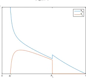
Figures 3, 4 and 5 plot the allocation of High-type and Low-type capital against Rb if 1 A
L < AH,
AL < 1 AH and AL < AH < 1, given = 0.5. The figures confirm that the emergence of a bubble
misallocates capital only if Rb< A
L. We can state the following Proposition.
PROPOSITION 1: A necessary condition for bubbles inducing a misallocation of factors is Rb< A L.
We also want to examine how the bubble affects the aggregate accumulation of capital, the output and the welfare of the economy.
PROPOSITION 2: The emergence of a bubble always reduces aggregate output and capital. The effect on aggregate consumption can be positive only if AH < 1.
The proof of Proposition 2 is in Appendix 1. Figures 6, 7 and 8 plot the steady state values of total output and consumption against Rb, given = 0.5. In this model, a bubble is always contractionary. This result
does not only derive from the typical crowding-out effect. The model adds an additional contractionary effect associated with the misallocation of factors. However, a bubble may still increase aggregate consumption, but only when the economy is dynamically inefficient.30
Finally, we can analyze how the identity of the investor that issues bubbly debt influences the aggregate economy.
PROPOSITION 3: An increase in always reduces aggregate output and capital. The effect on aggre-gate consumption can be positive only if AH< 1.
Proposition 3 is proved in Appendix 2. Intuitively, when Low productivity investors issue a larger share of unsecured notes, factors are misallocated and output is lower. In addition, since Low-type investors earn lower returns, a larger share of the workers’ future endowment must be allocated to the repayment of bubbly debt. This, eventually, reduces the total stock of capital.
To conclude, the model described here adds a new dimension to existing theories of rational bubbles. Bubbles do not only affect the aggregate accumulation of capital, they also have a re-allocation effect. Productive factors can be crowded out from specific sectors to be re-allocated to others. For a given interest rate, the effect of a bubble depends on this re-allocation of factors. In particular, the cost of a bubbly episode may be higher if it involves a large misallocation of capital towards low productive sectors.
This model, however, still does not tell us which investors would have an advantage in the issuing of bubbly debt. In addition, the contraction in output is always associated with a reduction in the stock of capital. In the next section, I will introduce some risk in the activity of the investors - which will affect their life expectancy on the market and, thereafter, their ability to maintain a bubbly scheme and accumulate capital over time. I will show that a bubble can boost aggregate capital accumulation even if that induces a misallocation of factors and a decrease in total production.
4 Credit Bubbles and Misallocation in a Model with Risky
Invest-ments
In this section I will extend the previous model by introducing a mechanism which predicts the misallocation equilibrium in a unique way. Importantly, the same mechanism will also open the doors for capital accumula-tion even if the bubble is contracaccumula-tionary. Here, investors will live for more than two periods but they will face some risk in their investment activity which will affect their life expectancy on the market and, thereafter, their ability to maintain a bubbly scheme and accumulate capital over time. In addition, workers will now supply labor and make an intertemporal consumption choice when young.31 All agents are assumed to be
risk neutral.
I will describe the problem faced by workers and investors in the following subsections. Note that, for simplicity, agents behave as if bubbles were deterministic. In looking at the dynamics, I will assume that the shocks to the system are unexpected.
4.1 OLG Workers
Workers live for two periods as in the previous version of the model. However, they now choose their total labor supply when young and their consumption in both young and old periods, by maximizing the following utility:
log (cY,t) 'ht+ log (cO,t+1) (26)
subject to cY,t= wtht lt+1and cO,t+1= Rt+1lt+1, where lt+1denotes lending in the credit market. For
simplicity I assume that the disutility from working is linear. The solution to the problem gives the aggregate supply of labor and lending:
ht= 2 ' (27) lt+1= 1 2wtht= wt '. (28)
4.2 Risky Investments
Investors are still grouped into two categories of mass one - High-type and Low-type - but they now live for more than two periods. Specifically, each investor has an i.i.d. probability of surviving in each period t. Then, in each period a mass (1 )of old investors leave the market and the same number of new investors enter the market with endowment e.32 Similarly to the previous section, the investors want to maximize
their consumption in their last period of life.33 Then, in all the previous periods, they will always reinvest
and continue to accumulate capital.
Again, the investors have a storing technology that will allow the installation of a specific kind of capital to rent in the following period to High-type or Low-type production. Unlike the activities described in the previous section, here the storing activity is risky. In particular, with respective probabilities (1 "H) and
(1 "L), the storing can fail and the investor can end up with no capital in the following period. I make the
assumption that these shocks are idiosyncratic and not insurable.
Production functions are now Cobb-Douglas combining capital and labor:
Ajkj,t↵h1 ↵j,t f or j2 {H, L} . (29)
I make the following assumptions: ASSUMPTION 2: "H< "L.
32Borrowing banks are modeled in a similar fashion in the model of bank runs described by Gertler and Kiyotaki (2015). 33Note that the same decision would derive if investors maximized a linear utility over consumption in different periods,
P1
ASSUMPTION 3: "↵
HAH > "↵LAL.
Assumption 2 states that the probability of failing is higher for an H-type investor. Nonetheless, Assump-tion 3 confirms that the overall H-type productivity is still higher. These premises describe an environment in which higher productivity sectors are also riskier. Conversely, low productive sectors offer more stability over time. Then, the two types of investment offer a different combination in the risk-return spectrum.
An investor m, of type H or L, raises external funding in the credit market and faces a similar borrowing constraint:
Rt+1dSm,t+1 MRKj,t+1"jim,t+1f or j2 {H, L} , (30)
where dS
m,t+1and im,t+1are secured debt and investment. That is to say, an investor of type j can secure his
borrowing up to a fraction of his expected capital income. The investors can also expand their borrowing by issuing bubbly debt. At this point, a further restriction is imposed:
ASSUMPTION 4: A debt contract can be exchanged as long as the issuer has positive equity.
Assumption 4 comes with an important implication: when an investor fails or dies, all the bubbly notes that he has issued will burst.34 This is a more accurate description of what happens in the real world where
tradable securities fail automatically with their issuers’ failure, or where financial institutions issue short-term notes which are rolled over under the same roof. Assumption 4 introduces a gap in the expected duration of H-type and L-type activities. It is worth pointing out that, given that H-type investors experience a shorter life expectancy on the market, they have a lower probability of rolling over a bubbly scheme.
4.3 Equilibrium and Steady State Solutions
The equilibrium in the economy is now defined as follows:DEFINITION: A competitive equilibrium is a list of consumption, lending, secured and unsecured debt, capital, labor, and prices such that:
(i) Young workers maximize their utility (26) by choosing ht and lt+1. Old workers consume Rtlt
(ii) An investor m of type j who is still active in the market in period t chooses im,t+1, lm,t+1U and dSm,t+1,
given dU
m,t+1 and prices (Rt+1, M RKj,t+1), maximizing profits in the last period of his life 1 X q=1 (1 ) q 1"j⇥M RKj,t+qim,t+q Rt+q dSm,t+q lUm,t+1 ⇤ f or j2 {H, L} (31)
subject to budget constraint
cm,t+ im,t+1+ lUm,t+1= M RKj,tim,t RtdSm,t+ dSm,t+1+ dUm,t+1, (32)
borrowing constraint (30) and resource constraints dS
m,t+1 M RKj,tim,t RtdSm,t+ dUm,t+1 and lm,t+1U 0.
An investor who dies in period t, consumes his final income cm,t= M RKj,tim,t Rt dSm,t lUm,t , while an
investor who fails leaves the market with no final consumption (iii) Factors are paid at their marginal productivity:
wt= (1 ↵) AH ✓ kH,t hH,t ◆↵ = (1 ↵) AL ✓ kL,t hL,t ◆↵ (33) M RKj,t= ↵Aj ✓h j,t kj,t ◆1 ↵ f or j2 {H, L} (34) with kj,t= "j ´ m2jim,tf or j2 {H, L}
(iv) Agents hold consistent beliefs about the path of dU
j,t+1f or j2 {H, L}
(v) All markets clear in every period.
As described in the previous section, the necessary condition to have bubbles misallocating resources is that both borrowing constraints are binding. Therefore, I make the following assumption.
ASSUMPTION 5: Rt+1< "LM RKL,t+18 t.35
Note that Assumption 5 implies Rt+1< "HM RKH,t+1 a fortiori. All investors will try to borrow until
their constraints bind and only the workers will lend in the credit market.
I begin by characterizing the steady state equilibria of the economy. Without bubbles in the economy, the steady state interest rate is:36
R⇤= 2 ↵
1 ↵. (36)
The previous section described bubbly debt equilibria as possible if Rb was lower than the growth rate
of the economy. This was possible because a debt security could also be exchanged after the death of the issuer. Here a bubbly scheme will burst if the issuer dies or fails, which means that in a steady state with
35The condition is on variables endogenously determined in the model. Therefore, it implicitly sets restrictions on parameters
so that all the equilibria we will characterize (with or without bubbles) respect the inequality.
36We can solve by plugging (33) in
R⇤w ' = ↵ ⇣ AHk↵Hh1 ↵H + ALkL↵h1 ↵L ⌘ . (35)
bubbles, High-type and Low-type investors cannot promise a return higher than "H and "L.37 From now
on, I will make the following assumption: ASSUMPTION 6: "H R⇤< "L.
Assumption 6 implies that only L-type investors can run a bubbly scheme in steady state. By backward induction, only L-type investors can credibly initiate a bubbly scheme because their survival rate in the market is higher given a lower probability of failure. A rational bubbly scheme relies on the expectation that the agents will continue to buy in the long run. Borrowers with riskier projects have a lower probability of survival and cannot sustain a long term pyramid scheme. In this course of event, a bubble will necessarily prompt the misallocation of resources from higher to lower productive borrowers. The interest rate Rb in
this bubbly equilibria will be such that R⇤ Rb " L< 1.
The dynamics of aggregate capital can now be set out in both sectors:
kH,t+1= "H ⇢ (1 ) e + (1 ) ↵ 1 ↵wthH,t+Rt+1 ↵ 1 ↵wt+1hH,t+1 (37) kL,t+1= "L ⇢ (1 ) e + (1 ) ↵ 1 ↵wthL,t+Rt+1 ↵ 1 ↵wt+1hL,t+1 + "L ⇢ lt+1 Rt+1 ↵ 1 ↵wt+1ht+1 Rt ✓ lt Rt ↵ 1 ↵wtht ◆ . (38)
The curly braces refer to the H-type and L-type aggregate investments in time t. Newly-arrived investors of both types invest their endowment e. Pre-existing investors who remain in the market in period t, on aggregate reinvest their income: (1 ) M RKj,tkj,t= (1 )1 ↵↵ wthj,tf or j2 {H, L}. All investors in the
market will also invest all external funding they are able to raise in the credit market: Rt+1M RKj,t+1kj,t+1=
Rt+1
↵
1 ↵wt+1hj,t+1f or j2 {H, L}. In addition, L-type investors can invest the rent they obtain from issuing
unsecured debts. In the last line we can see that the rent is given by the portion of current unsecured debt that is not allocated to the repayment of past unsecured debt. In an equilibrium with no bubbles, the rent is equal to 0. Finally, both types of aggregate investments are fractioned by the respective storage survival rate.
In steady state the two equations can be simplified: kH= "H ⇢ (1 ) e + (1 ) + Rb ↵ 1 ↵whH (39) kL= "L ⇢ (1 ) e + (1 ) + Rb ↵ 1 ↵whL+ 1 R b Rb R⇤ Rb w ' . (40) 37
Substituting into (33), the steady state labor allocation is finally obtained as a function of w : hH =⇣ (1 ) e w (1 ↵)"↵ HAH ⌘1 ↵ h (1 ) +Rb i ↵ 1 ↵w (41) hL= (1 ) e + 1 Rb Rb R⇤ Rb w' ⇣ w (1 ↵)"↵ LAL ⌘1 ↵ h (1 ) +Rb i ↵ 1 ↵w . (42)
It is easy to see that in the bubble-free equilibrium, i.e. when Rb = R⇤, the allocation of capital and labor
is driven by the aggregate productivities "↵
HAH and "↵LAL. Since the latter is smaller, High-type investors
receive more capital and labor. The rise of a bubble misallocates factors in favor of the Low-type investors. The following Proposition can now be stated.
PROPOSITION 4: A bubble always reduces total output.
A formal proof is provided in the Appendix. Intuitively, it would seem that a bigger Rb increases the
amount of unsecured debt in the economy, which would raise both the misallocation and the crowding-out of lending. As expected, bubbles in this section are always contractionary. Nevertheless, this does not necessarily imply a reduction in the aggregate stock of capital as it did in the previous section.
PROPOSITION 5: There exist steady state equilibria with bubbles in which aggregate capital increases. The proposition is proved in Appendix 4. The bubbly episodes preceding a financial crisis are typically characterized by a fast accumulation in capital. In particular, in the years prior to 2008 we saw a boom in the housing sector. The original theory of rational bubbles could not explain this phenomenon. In Tirole’s framework, a bubble would reduce capital when the economy is dynamically inefficient. The addition of credit constraints in the new literature on rational bubbles, has introduced a new class of bubbly equilibria: by improving the intratemporal allocation of funding, bubbles can boost output and capital. In this section I in-troduced a further type of bubbly episode. This bubble reduces output and increases capital by misallocating resources towards low productive sectors which, nonetheless, have a higher propensity to accumulate. Our result is driven by the assumption that low productive sectors have a lower fundamental risk. Interestingly, the model predicts the emergence of non-fundamental risk in sectors that are fundamentally more stable.
4.4 The Dynamics of the Model without Nominal Rigidities
This section will set out the simulated dynamics of the model when the system is hit by unexpected shocks to the interest rate Rt. I will start by analyzing the transition dynamics between the bubble-free steady state,
characterized by R⇤, and the bubbly steady state with Rb= " L.
The model is solved numerically. The share of capital is in line with data from developed countries: ↵ = 0.35. The selection of the remaining parameters respects the assumptions set out in the previous section. Specifically, I set AH = 1.9, AL = 1.1, "H = 0.13, "L = 0.6, = 0.75, = 0.4, e = 0.001, ' = 1.
is low enough so that Assumption 5 is respected. Similarly, the choice for , "H and "L is made to meet
Assumption 6. In particular, to confirm Proposition 5, "H is set sufficiently small relatively to "L that a
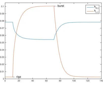
reallocation of funding towards L-type investors would boost capital accumulation. In this simulation the economy starts from a bubble-free steady state: in period 11 the interest rate rises from R⇤ to Rb= "
L; in
period 71 the bubble bursts and the return converges to R⇤.
Figure 9 and 10 report the path for the allocation of capital and labor. While the reallocation in the labor market is symmetrical, given a fixed total labor supply, we can see how the increase in the amount of L-type capital overtakes the reduction in H-type capital when the bubble appears. This can also be observed in the path for aggregate capital presented in Figure 11. However, the rise in the aggregate stock of capital is not reflected in a long run expansion in output. Total production gradually decreases at the emergence of the bubble, and only returns to its initial steady state level when the bubble bursts (Figure 12).
An apparent drawback to this model is the timing of the expansion and the recession. Bubbly times are generally expansionary, at least in the short run; recessions typically start at the burst of the bubble. For this reason, recent papers have introduced a productive efficiency role for rational bubbles. In the next section I will propose a different channel by which an increase in asset prices produces a positive effect on output. I will add nominal rigidities to our environment and show how a rise and drop in returns can be associated with both short-run and long-run effects. A nominal rise in the credit market return, given price rigidities, will imply a higher demand and an optimal increase in the labor supply. In the long run, when prices can adjust, the demand effect will be absorbed and only the emergence of a bubble can support high real returns.
4.5 The Dynamics of the Model with Nominal Rigidities
To introduce demand effects associated with nominal rigidities, I will now assume that firms produce dif-ferentiated goods and compete in a monopolistic fashion. Specifically, agents in the economy consume two perfectly substitutable composite goods produced by firms of type H and L:
Yt= YH,t+ YL,t= ˆ n2H y ⌘ 1 ⌘ n,t dn ⌘ ⌘ 1 + ˆ n2L y⌘⌘1dn ⌘ ⌘ 1 (43) for ⌘ 1, where yn,t is the output of a single firm, while YH,t and YL,t are the aggregate output from
one. The implied composite prices are: Pt= PH,t= PL,t= ˆ n2H p1 ⌘n,t dn 1 1 ⌘ = ˆ n2L p1 ⌘n,t dn 1 1 ⌘ . (44)
In equilibrium, the two composite prices must be equal, given that the two goods are perfect substitutes. In what follows, all variables in nominal terms will have a superscript N. In order to keep the study of the dynamics as simple as possible I will keep the assumption that shocks to the system are unexpected.
I assume young workers own the monopolistic firms and earn their profits. Then, they maximize:
log (cY,t) 'ht+ log (cO,t+1) (45)
subject to cY,t= w N t Pt ht+ ⇧Nt Pt lt+1 and cO,t+1= ⇣ RN t+1PPt+1t ⌘
lt+1. lt+1 denotes the real amount of lending
in the credit market. wN
t and ⇧Nt respectively denote the nominal wage and profits. RNt+1 is the nominal
return. Young workers choose the following optimal supply of labor and lending:
ht= wN t ht ⇧N t + wtNht 2 ' (46) lt+1= 1 2 ✓wN t Pt h +⇧ N t Pt ◆ = wt '. (47)
It is worthy to note that the labor supply increases with the relative share of labor income to profits. This is crucial to generating demand effects in the economy.
Each firm n maximizes its profits
pn,tAjk↵n,th1 ↵n,t QNj,tkn,t wNt hn,t f or j2 {H, L} (48)
given prices QN
j,t and wNt , and demand constraint yn,t =
⇣P
n,t
Pt
⌘ ⌘
Yj,t. Note that the price of capital Qj,t
can now be different from the marginal return on capital MRKj,t, given the presence of monopolistic rents.
I assume that the price of a good is set one period in advance: as long as no unexpected shock hits the economy, a firm will set the price at a constant markup ⌘
⌘ 1 over its marginal cost. Optimal capital and
labor demand will be such that
n,tpn,t↵Aj ✓ hn,t kn,t ◆1 ↵ = QNj,tf or j2 {H, L} (49) n,tpn,t(1 ↵) Aj ✓k n,t hn,t ◆↵ = wNt f or j2 {H, L} , (50)
where n,t is the portion of revenues allocated to the payment of factors. When a firm can optimally set his
price, it must be n,t= ⌘ 1⌘ 8 n38. The aggregate tin period t can be defined as
t= H,tYH,t
Yt
+ L,tYL,t
Yt
, (51)
where H,tand L,tare the respective shares of High and Low type firms. Fluctuations in twill be associated
to demand effects. The incomes and profits in the economy can be rewritten as a function of tand aggregate
output YN
t : QNH,tkH,t+ QL,tN kL,t = t↵YtN, wtNht= t(1 ↵) YtN and ⇧Nt = (1 t) YtN. Then, from (46),
I can express the labor supply as an increasing function of t:
ht=
(1 ↵) t
(1 t) + (1 ↵) t
2
'. (52)
The workers are willing to increase their labor supply when the share of revenues allocated to the payment of factors is larger.
The dynamics of capital is still described by equations (37) and (38); in Appendix 5 I report the steady state solutions for this economy. In this version of the model, the return is subject to two shocks of different nature. First, as in the previous subsection, the interest rate can change because of the emergence and burst of a bubble. Second, a monetary shock can induce a demand effect because of the presence of nominal rigidities.
From the binding borrowing constraint, we can express the realized nominal return of the secured notes RN
t as a function of a natural rate ¯Rt, a gap in the repayment of factors
✓ tYt ⌘ 1 ⌘ Y¯t ◆ and inflation⇣ Pt Pt 1 ⌘ : RNt = Rt ✓ Pt Pt 1 ◆ = ¯Rt ⌘ 1tYt ⌘ Y¯t ! ✓ Pt Pt 1 ◆ . (53)
In Appendix 6 I describe how to obtain the formula above. In the previous subsection I analyzed the system when hit by unexpected shocks to ¯Rt. These shocks were associated with the start or end of a bubble scheme.
Every time, it must be:
¯ Rt 2 ↵ 1 ↵ (⌘ 1) (1 ↵) 1 + (⌘ 1) (1 ↵) ¯ wt wt 1 . (54)
In particular, the condition holds with equality when there is no bubbly debt in the economy. In this subsection I will consider also the effect of a shock to✓ tYt
⌘ 1 ⌘ Y¯t ◆ ⇣ Pt Pt 1 ⌘ . In a deterministic envi-ronment it must be ✓ tYt ⌘ 1 ⌘ Y¯t ◆
= 18 t. However, by assuming that prices must be set one period in advance, an unexpected change in ✓ tYt ⌘ 1 ⌘ Y¯t ◆
is possible. Therefore, a variation in RN
demand effect. For example, a rise in the credit market return, given price rigidities, would trigger an increase in demand, which can only be satisfied by a reduction in the firms’ markup. This encourages the supply of labor, from equation (52) and, ultimately, boosts the returns on capital and relax the borrowing constraint. It is relevant to note that an increase in the real return Rtcan be associated with an economy contraction
when driven by a change in ¯Rt, and an economy expansion when driven by a positive demand shock.
I will simulate the dynamics of the model when the system is hit by a positive and a negative demand shock. In a first simulation, I assume that the shocks are absorbed in the long run without the emergence or burst of a bubble. In particular, I assume that the shocks imply a permanent change in the nominal return, but an adjustment in the inflation rate brings the real return back to its original steady state. In a second simulation, I assume that, after the original positive (negative) demand shock, prices do not adjust and a bubble arises (bursts).
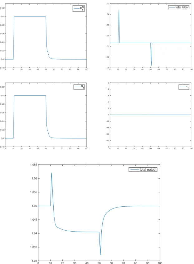
The model is solved numerically. ⌘ is set equal to 11, in order to have a 10% markup. The remaining parameters are similar to the ones chosen in the previous subsection: ↵ = 0.35, AH = 1.9, AL = 1.1,
"H = 0.13, "L = 0.6, = 0.75, = 0.45, e = 0.001. In both simulations, I assume that in period 11 RNt
increases from R⇤= 0.42to 0.43; then, from period 51 the rate RN falls back to 0.42.
Figure 13 reports the results of the first simulation. In this case, there are no bubbles appearing in the economy. The sudden increase in RN
t triggers a demand effect in the time of the shocks, given that prices
are rigid. The real return reacts in an identical way only in the time of the unexpected shocks. Starting from the periods that follow the positive (negative) shock, the inflation rises (drops) and the real interest rate goes back to the bubble-free steady state level. The demand shocks produce a temporary real effect. In the period of the increase (fall) in RN
t , the labor supply reacts in a positive (negative) way. The total output
is boosted in period 11 because of the higher labor supply. Then it gradually goes back to its original steady state. The opposite dynamics is triggered from period 51 on. Note that Rt and ⇡t do not follow a smooth
path after the shocks. For example, Rtfalls below the steady state level after the initial positive shock. The
reason can be seen in equation (54): a positive demand shock that boosted the output at time t 1, induces a reduction in ¯Rtgiven an increase in the total lending.
In Figure 14 I present the results of the second simulation. Here, prices do not adjust after the initial demand shocks. Then, the higher (lower) real return is supported by the emergence (burst) of a bubble. Such a dynamics may be justified by a coordination on zero-inflation equilibria.39 Therefore, inflation is stationary
while the total labor reacts in period 11 and 51 as in the previous scenario. This experiment allows me to reproduce a situation in which the initial boom in market returns induces an immediate positive demand effect which gradually vanishes and gets replaced by a long run misallocation of factors. The output boom in
period 11 turns into a recession in the following periods. Similarly, the output drop in period 51 is followed by an expansion that brings the system back to the initial steady state.
The exercise proposed in this subsection provides a potential interpretation for the dynamics of credit, output and TFP that we observed in the recent times of low inflation. While the initial boom is triggered by a positive demand effect, the reduction in TFP is induced by the emergence of a bubble. Although the two effects are driven by two different types of shocks, they are both associated with higher market returns. In the next section, I will study the policy implications suggested by the model.
4.6 Policy Implications
By way of a final contribution, this paper looks at the policy prescriptions implicit in the model. In the model, a monetary authority, controlling the nominal value of the secured credit contracts, can effectively close the gap between the output Ytand its natural level ¯Yt. However, this has no effect on ¯Rt.
In order to influence the real return ¯Rtand the allocation of factors, other instruments are needed. Given
the simple structure of the framework set out here, an optimal allocation of factors is one in which all credit and labor are assigned to high productive investors.40 In this context, a planner would promote a reallocation
by discouraging L-type activity. A simple route to this would be to tax the capital income of the L-type investors. In particular, for a proportional tax ⌧L,t, L-type investors would prefer to lend to H-type investors
if
(1 ⌧L,t) "LM RKL,t< Rt; (55)
i.e., if the equilibrium interest rate was higher than the expected return from the L-type investment.41 In
the following I assume ⌧L,t is large enough to allow the condition to be respected.
Bubbles are still possible even if high productive borrowers obtain the entire funds. In a long run steady state, the social planner would like to target the return ¯Rg that maximizes the aggregate welfare of the
economy: log 1 2 ✓ 1 ↵⌘ 1 ⌘ ◆ YH R¯g + log 1 2R¯ g✓1 ↵⌘ 1 ⌘ ◆ YH R¯g + (1 ) ↵⌘ 1 ⌘ YH R¯ g + ¯Rg 1 1 R¯ge. (56)
The first line refers to the utility of the workers; the second line reports the utility of the H-type investors and L-type investors. Given an optimal allocation of factors, a bubbly scheme is certainly contractionary
40Since "↵
HAH> "↵LAL, it is always "HM RKH,t> "LM RKL,t. 41
- the only effect is to crowd-out H-type capital. However, by transferring resources from younger to older agents, the consumption of the latter may increase if the economy is dynamically inefficient.
A social planner can target an optimal rate ¯Rgt+1 by imposing its monopoly on the creation of bubbly
notes. The planner would set a cap on the debt creation by the private sector. It must be: dH,t+1 ¯Rg
t+1
↵YH,t+1 R¯gt+1 8 t. (57)
In addition he can directly introduce bubbly notes when ¯Rgt+1is larger than the bubble-free rate R⇤ t+1 and
the workers have extra resources to lend. An optimal amount of unsecured notes dU t+1 R¯
g
t+1 can be issued
by a government in the form of government bonds,42or by a central bank in the form of bank notes. Clearly,
the fraction that the planner earns as a rent should be transferred to subsidize H-type investment.
5 Conclusions
Financial crises are typically preceded by a credit boom. According to a widespread view, the costs of a crisis originates in the sudden freezing of the credit markets. Recent contributions to the literature on rational bubbles associate these fluctuations in credit to bubbly episodes. In these papers, bubbles expand output and capital by improving the allocation of funding when productive agents are financially constrained. The burst of the bubble would then lead to a recession.
The evidence, however, shows that a rapid growth in credit promotes a misallocation of resources towards low productive industries. For example, housing and real estate sectors are the usual recipients of an increased share of capital in a credit boom. This paper shows how this phenomenon can be explained in the rational bubble framework. Here, investors with different productivities can borrow by pledging their future income as collateral or by repaying with future new debt issues. The key intuition for the misallocation result is that borrowing through unsecured debt does not require high productivity. Instead, a credit bubble favors those borrowers who have a low probability of exiting the market in the future and can maintain a long-lived scheme.
An important result of the theory is that bubbles can promote capital accumulation even if they are contractionary. Funding would be reallocated towards lower productive sectors which have a higher propensity for accumulation. This explains both the investment misallocation and the growth in capital stock that can be observed during a credit boom.
The implications of my framework stand in stark contrast to the recent literature on rational bubbles. A bubbly expansion in credit is harmful to the economy, not from the risk of a future collapse, but for the