DIETRICH STAUFFER1,2∗∗, PAULO M.C. DE OLIVEIRA2∗∗∗, SUZANA MOSS DE OLIVEIRA2, THADEU J.P. PENNA2and JORGE S. SÁ MARTINS3
1Institute for Theoretical Physics, Cologne University, D-50923 Köln, Germany (Permanent address) 2Instituto de Física, Universidade Federal Fluminense, Av. Litorânea, s/n – Boa Viagem, 24210-340 Niterói, RJ
3Colorado Center for Chaos and Complexity / CIRES, University of Colorado, Boulder CO 80309, USA
Manuscript received on November 22, 2000; accepted for publication on November 29, 2000.
ABSTRACT
The sexual version of the Penna model of biological aging, simulated since 1996, is compared here with alternative forms of reproduction as well as with models not involving aging. In particular we want to check how sexual forms of life could have evolved and won over earlier asexual forms hundreds of million years ago. This computer model is based on the mutation-accumulation theory of aging, using bits-strings to represent the genome. Its population dynamics is studied by Monte Carlo methods.
Key words:parthenogenesis, genome, menopause, testosterone, Monte Carlo simulation.
1. INTRODUCTION
Can physicists contribute to understand biological subjects? Since the first attempts by the Nobel lau-reate Schrödinger (1944), there were a lot of tenta-tive answers to this question, probably most of them useless. What particular knowledge can physicists bring to Biology? One particular tentative, biased answer for this second question is presented below. It is biased because it concerns just the authors’ tra-ditional line of research.
Critical phenomena appear in macroscopic physical systems undergoing continuous phase tran-sitions. An example is water crossing the critical temperature of 374◦C, above which one can no longer distinguish liquid from vapour. Another is a ferromagnetic material which loses its spontaneous magnetisation when heated above its critical
tem-∗Invited paper
∗∗Foreign Member of Academia Brasileira de Ciências (ABC) ∗∗∗Member of ABC
Correspondence to: Paulo M.C. de Oliveira E-mail: [email protected]
manufac-turing of artificial muscles, catheters which unblock arteries, microengines, etc.
These features have attracted the attention of physicists since more than a century. They dis-covered an also unusual behaviour concerning the mathematical description of such systems: the ap-pearence ofpower-laws, i.e. Q ∼ |T −Tc|−γ or C ∼ |T −Tc|−α, whereQis the quoted diverging quantity (compressibility or magnetic susceptibil-ity),C is the specific heat, and|T −Tc|measures how far the system is from its own critical point. The symbol∼represents proportionality. Critical
exponents likeγ,α, etc are characteristic of the cor-responding quantity,Q,C, etc.
The most interesting feature of these phenom-ena is the so-called universality: the precise val-ues of the exponentsγ,α, etc are the same for en-tire classes of completely different systems. For instance,α = 0.12 for both water and any
ferro-magnet in which ferro-magnetisation presents uni-axial symmetry. Also,γ =1.24 for both the water
com-pressibility and the magnetic susceptibility of the ferromagnetic material. Besides critical exponents, many other qualitative and quantitative character-istics of the various systems belonging to the same universality class coincide as well. In spite of having been observed much before, these coincidences re-mained unexplained until the work of Wilson (1971), three decades ago, who was awarded with the No-bel prize because of this work (see also: Wilson & Kogut 1974, Wilson 1979). The key concept needed to understand this phenomenon is the decaying of correlations with increasing distances. Suppose one picks two points inside the system, separated by a distancex. How much a perturbation performed at one of these points will be felt at the other? The correlationI between these two points is a measure of this mutual influence, and generally decays for larger and larger values ofx, according to the expo-nential behaviour
I ∼exp(−x/ξ )
(for non critical situations), (NC)
whereξ is the so-called correlation length. Would
one take two points distant from each other a dis-tancex larger than ξ, the correlationI would be negligible. This means that one does not need to study the macroscopic system as a whole, with its enormous number of component units: it is enough to take a small piece of the system with linear di-mensions of the same order asξ (for instance, a sphere with radius, say, 10ξ). Once one knows, for instance, the specific heat of this small piece, that of the whole system is obtained by a simple volume proportionalityC∼V orQ∼V.
However, the nearer the system is to its critical point, the larger isξ, and the larger is the “small” piece representing the whole, i.e. ξ ∼ |T −Tc|−ν. Justatthe critical point, one can no longer break the system into small pieces: the macroscopic critical behaviour of the system is no longer proportional to its volume. Instead, critical quantities become non-linear, non-extensive, and behave asQ∼Vγ or C ∼ Vα, where
γ = γ /3ν, α = α/3ν, etc. Also, the above exponential form (NC) forI concerns only the dominating decay valid for a finite ξ. Atthe critical point whereξ → ∞, however,
other sub-dominating terms enter into the scene, i.e.
I ∼x−η
(for critical situations), (C)
whereηis another critical exponent.
Both forms (NC) and (C) mean that correla-tions decay for larger and larger distances. The im-portant conceptual difference is that in (NC) they de-cay much faster, according to a characteristic length scaleξ above which correlations become negligi-ble. On the opposite, there is no characteristic length scale in the critical case (C): correlations are never negligible even between two points very far from each other, inside the system. Thus clusters and holes are observed at all sizes, a crucial property e.g. for electrophoresis.
property: most microscopic details of the system are irrelevant in what concerns its critical behaviour, since large distances dominate the scenario. That is why water compressibility presents exactly the same critical exponentγ as the magnetic suscepti-bility of any uni-axial ferromagnet, as well as the same values for the other exponents α, ν, η, etc, and thus the same critical behaviour. Not only wa-ter and such ferromagnetic mawa-terials, but also any other natural or artificial system which belongs to the same (huge) universality class. One example of such mathematical toys is the famous Ising model: each point on a regular lattice holds a binary variable (a number 0 or 1), and interacts only with its neig-bouring sites. No movement at all, no molecules, no atoms, no electrons interacting through compli-cated quantum rules. The only similarities between this toy model and real water are two very general ingredients: the three-dimensionality of the space and the one-dimensionality of the main variables involved (the numbers 0 or 1 within the toy, and the liquid-vapour density difference within water, also a number, as opposed to a three-dimensional vector). Nevertheless, one can use this very simple toy in order to obtain the critical behaviour common to all much more complicated systems belonging to the same universality class.
However, even the study of these toy models is far from trivial, due to the already quoted impos-sibility of breaking the system into small, separate pieces. Thus, the main instrument is the computer, where one can store the current state of each unit, i.e. a number 0 or 1, into a single bit of the mem-ory. By programming the computer to follow the evolution of this artificial system time after time, i.e. by repeatedly flipping 0s into 1s (or vice-versa) according to some prescribed microscopic rule, one can measure the various quantities of interest. Note that this approach has nothing to do with the numer-ical solution of a well posed mathematnumer-ical problem defined by specific equations. Instead, the idea isto simulatethe realdynamicalbehaviour of the sys-tem on the computer, andto measurethe interesting quantities. During the last half century, this “almost
experimental” technique was tremendously devel-oped by the (now-called) computational physicists, a fast growing scientific community to which the au-thors belong (Stauffer & Aharony 1994, de Oliveira 1991, Moss de Oliveira et al. 1999a).
Biological evolution (Darwin 1859) also pres-ents the same fundamental mathematical ingredi-ents which characterise physical critical systems: the power-laws. A lot of evidences are known, today (see, for instance, Kauffman 1993, 1995, Bak 1997). A simple and well known example is the numberAof still alive lineages within an evolving population: it decays in time according to the power-lawA∼t−1, where the exponent−1 can be exactly obtained from
the coalescence theory (see, for instance, Excoffier 1997). According to this, after many generations, all individuals of the population are descendents of a single lineage-founder ancestor. The number of generations one needs to wait for this coalescence is proportional to the number of founder individuals, due to the value−1 of the exponent. Also, during the
whole evolution of the population, the numberEof already-extinct lineages withnindividuals behaves asE∼n−0.5, where the new exponent−0.5 is also
exactly known. The interesting point is that these exponents are universal, i.e. their precise values do not change for different microscopic rules dic-tating how individuals die, how they are born, etc. Another simple example is the evolution of a reces-sive disease: the frequency of the recesreces-sive gene among the evolving population also decays in time as a power-law, thuswithout a characteristic ex-tinction time. Due to this particular mathematical decaying feature, the recessive gene extinction is postponed forever (Jacquard 1978). An explanation for the narrow relation between biological evolution and critical dynamics is presented by de Oliveira (2000).
dur-ing the last half decade, and was applied to many different biological problems involving aging, al-ways within the general interpretation above:a very simple model supposed to reproduce the univer-sal features of much more complicated, real phe-nomena.
Senescence, or biological aging, can mean many things; for computer simulations it is best de-fined as the increase of mortality with increasing age. It seems not to exist for bacteria, where even the concept of death is difficult to define, but for humans as well as for other organisms (Vaupel et al. 1998) this rapid increase of the probability to die, after childhood diseases are overcome, is well known. Fig. 1 shows typical human data for a rich country.
The reasons for aging are controversial (Watch-er & Finch 1997, see also the whole special issues of La Recherche: July/August 1999 and Nature: November 9th, 2000). There may be exactly one gene for longevity, or senescence comes from wear and tear like for insect wings and athlete’s limbs, from programmed cell death (apoptosis - Holbrook et al. 1996), from metabolic oxygen radicals de-stroying the DNA (see for instance Azbel 1994), or from mutation accumulation (Rose 1991). The computer simulations reviewed here use this last as-sumption, which does not exclude all the other rea-sons. For example, the oxygen radicals may produce the mutations which then accumulate in the genome transmitted from one generation to the next. Ex-cept if stated otherwise, the mutations here are all detrimental and inherited.
After a short description of the model in section 2, we deal in section 3 with the question whether sexual reproduction was better or worse than asexual reproduction hundreds of million years ago when sex appeared, while section 4 tries to explain why today’s women live longer than men and have meno-pause. Section 5 reviews other aspects, and Section 6 gives a short summary.
A more detailed account, but without the results of 1999 and 2000 emphasized here, is given in our book (Moss de Oliveira et al. 1999a).
2. THE PENNA MODEL
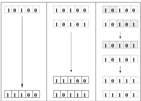
In the original asexual version of the Penna model (Penna 1995) the genome of each individual is rep-resented by a computer word (bit-string) of 32 bits (each bit can be zero or one). It is assumed that each bit corresponds to one “year” in the individual lifetime, and consequently each individual can live at most for 32 “years”. A bit set to one means that the individual will suffer from the effects of a dele-terious inherited mutation (genetic disease) in that and all following years. As an example, an individ-ual with a genome 10100...would start to become sick during its first year of life and would become worse during its third year when a new disease ap-pears. In this way the bit-string represents in fact a “chronological genome”. The biological motiva-tion for such a representamotiva-tion is, for instance, the Alzheimer disease: its effects generally appear at old ages, although the corresponding defective gene is present in the genetic code since birth.
The extremely short size of the 32 bit-string used in the model would be totally unrealistic if all our genes were related to life-threatening diseases. However, among the average number of 108units we
have in our real genome, only around 104to 105units
play a functional role. Moreover, only a subgroup of these will give rise to a serious disease at some moment of the individual lifetime. Besides, qual-itatively there was no difference when 32, 64 and 128 bits were taken into account (Penna & Stauffer 1996).
One step of the simulation corresponds to read-ing one bit of all genomes. Whenever a new bit of a given genome is read, we increase by one the indi-vidual’s age. The rules for the individual to stay alive are: 1) The number of inherited diseases (bits set to 1) already accumulated until its current age must be lower than a thresholdT, the same for the whole population. In the example given above, ifT =2
environ-0.0001 0.001 0.01 0.1 1
0 20 40 60 80 100
mor
tality function
age
Fig. 1 – Male (+) and female (x) mortality functions in the USA, 1991-1995; from J.R. Wilmoth’s Berkeley Mortality Database demog.berkeley.edu/wilmoth/. The straight line through the male data indicates the expo-nential increase with age (Gompertz law). These mortality functions are defined as−dlnS(a)/dawhereS(a) is the probability to survive up to an age ofayears.
ment can support andN (t )is the current population size. We usually considerNmaxten times larger than the initial populationN (0). At each time step and for each individual a random number between zero and one is generated and compared withV: if it is greater thanV, the individual dies independently of its age or genome. The smaller the population size is, the greater is the probability of any individual to escape from this random killing factor.
If the individual succeeds in staying alive un-til a minimum reproduction age R, it generatesb offspring in that and all following years (unless we decide to set also some maximum reproduction age). The offspring genome is a copy of the parent’s one, except forMrandomly chosen mutations introduced at birth. Although the model allows good and bad mutations, generally we consider only the bad ones.
backward ones (reverse mutations deleting harmful ones - Pamilo et al. 1987).
The sexual version of the Penna model was first introduced by Bernardes (1995, 1996), followed by Stauffer et al. (1996) who adopted a slightly differ-ent strategy. We are going to describe and use the second one (see also Moss de Oliveira et al. 1996). Now individuals are diploids, with their genomes represented by two bit-strings that are read in paral-lel. One of the bit-strings contains the genetic infor-mation inherited from the mother, and the other from the father. In order to count the accumulated number of mutations and compare it with the thresholdT, it is necessary to distinguish between recessive and dominant mutations. A mutation is counted if two bits set to 1 appear at the same position in both bit-strings (inherited from both parents) or if it appears in only one of the bit-strings but at a dominant posi-tion (locus). The dominant posiposi-tions are randomly chosen at the beginning of the simulation and are the same for all individuals.
The population is now divided into males and females. After reaching the minimum reproduction ageR, a female randomly chooses a male with age also equal to or greater thanRto breed (for sexual fidelity see Sousa & Moss de Oliveira 1999). To con-struct one offspring genome first the two bit-strings of the mother are cut in a random position (crossing), producing four bit-string pieces. Two complemen-tary pieces are chosen to form the female gamete (recombination). Finally,mf deleterious mutations are randomly introduced. The same process occurs with the male’s genome, producing the male gamete withmmdeleterious mutations. These two resulting bit-strings form the offspring genome. The sex of the baby is randomly chosen, with a probability of 50% for each one. This whole strategy is repeated b times to produce the b offspring. The Verhulst killing factor already mentioned works in the same way as in the asexual reproduction.
A very important parameter of the Penna model is the minimum reproduction ageR. According to mutation accumulation-theory, Darwinian selection pressure tries to keep our genomes as clean as
possi-ble until reproduction starts. For this reason we age: mutations that appear early in life are not transmitted and disappear from the population, while those that become active late in life when we barely reproduce can accumulate, decreasing our survival probability but without risking the perpetuation of the species. One of the most striking examples of such a mech-anism is the catastrophic senescence of the pacific salmon and other species called semelparous: In these species all individuals reproduce only once in life, all at the same age. This can be easily imple-mented simply by setting a maximum reproduction age equal toR. After many generations, the inher-ited mutations have accumulated in such a way that as soon as reproduction occurs, individuals die. This explanation was given by Penna et al. (1995), using the Penna model (see also Penna & Moss de Oliveira 1995 and a remark from Tuljapurkar on page 70 in Wachter & Finch 1997).
3. COMPARISON OF SEXUAL AND ASEXUAL REPRODUCTION
3.1.Definitions
In this section we check which way of reproduc-tion is best: Sexual, asexual or something in be-tween. We denote as asexual (AS) and sexual (SX) the simulation methods described in the previous section, that means cloning of a haploid genome for AS, and crossover for diploid genomes with males and females separated for SX. Intermediate possi-bilities which will also be compared are apomic-tic parthenogenesis (AP), meioapomic-tic parthenogenesis (MP), hermaphroditism (HA), and mixtures of them. One could also group AS, AP and MP into asexual and HA and SX into sexual reproduction. Parasex, the exchange of haploid genome parts between dif-ferent bacteria, is not simulated here.
phe-nomena are overcome, is regarded as the best. We assume it would win in a Darwinian selection (see Stauffer et al. 2000 for some justification) if dif-ferent populations following these difdif-ferent ways of reproduction would compete against each other in the same environment, without any symbiosis or predator-prey relation between them.
AS and SX were defined already in the preced-ing section. For AP the diploid genome is copied without crossover, only mutations. For MP the diploid genome is crossed over, and one of the two resulting haploid bit-strings is randomly cho-sen, duplicated and mutated to form the new diploid genome. HA is similar to SX except that there is no separation into males and females; instead all of them can generate offspring and each individual se-lects randomly a partner from the whole population to exchange genome as in SX. Fig. 2 summarizes the four versions schematically.
In all the copying of genome (bit-strings), point mutations are assumed to happen with the same probability per bit. Thus typically for AS with a genome of 32 bits we assume one mutation per gen-eration for the whole genome, while for the diploid cases AP, MP, HA and SX we assume two. (We as-sume the same mutation rate for males and females in the Penna model simulations.) The birth rate is also assumed to be the same for all birth-giving in-dividuals. For example, for AS, AP, MP and HA we have four offspring per suitable individual and per year, while for SX we have four offspring per suitable female and per year. Thus the birth rate av-eraged over males and females is only two instead of four. And we have to find out whether this loss of a factor of two in the average birthrate for SX is overcome by advantages not contained in the other ways of reproduction.
(For HA as simulated by Stauffer et al. (2000) during one iteration some individuals have already aged by one “year”, while others have not yet aged. Results do not change much, see topmost data in Fig. 3 below, if now in one iteration we first let everybody age one time unit, and only afterwards partners are selected.)
3.2.Comparison without aging
The Redfield model (Redfield 1994) is an elegant model requiring much less computer time than the Penna model, but having no age structure. It is not a population dynamics model following the lifetime of each individual, but only simulates their proba-bilities to survive up to reproduction. The mortality increases exponentially with the number of muta-tions in the individual. For the sexual variant the number of mutations in the child is determined by a binomial distribution such that on average the child has as its own number of mutations half the number of the father, plus half the number from the mother. At birth, new mutations are added following a Pois-son distribution, for both AS and SX. Because of the lack of an explicit genome, the forms AP, MP, HA between AS and SX were not simulated.
This model triggered many publications in the physics literature since it originally made SX much worse than AS: The average mortality was about 25 percent for AS, and did not change when the simula-tion switched to SX. But still the males were eating the food away from the females. Actually, the male mutation rate is much higher than the female one, and when that was taken into account the mortality with SX became much higher than for AS (Redfield 1994).
However, the picture changed drastically when we took into account (Stauffer et al. 1996) that most hereditary diseases are recessive (acting only when both father and mother had them in their transmit-ted genome) and not dominant (acting already when only one of the two inherited bit-strings has them). Then the mortality decreased by about an order of magnitude, and SX became much better than AS. The same drastic improvement was found when for SX the females selected only males with few muta-tions.
domi-1 0 domi-1 0 0 1 0 1 0 1 0 1 0 0
0 1 1
1 1 0 1 0
0
0 1
1 0 1 0 1
1 0 1 0 1
1 0 1 1
1 1 1 0 1 1 1 1 1 0 0
1 0 1 1 1 1 0 0
1 1
Fig. 2a – Schematic representation of the genomic changes for AS, AP, MP (from left to right).
1.6e+07 1.7e+07 1.8e+07 1.9e+07 2e+07 2.1e+07 2.2e+07 2.3e+07
0 2000 4000 6000 8000 10000
n
umber
time
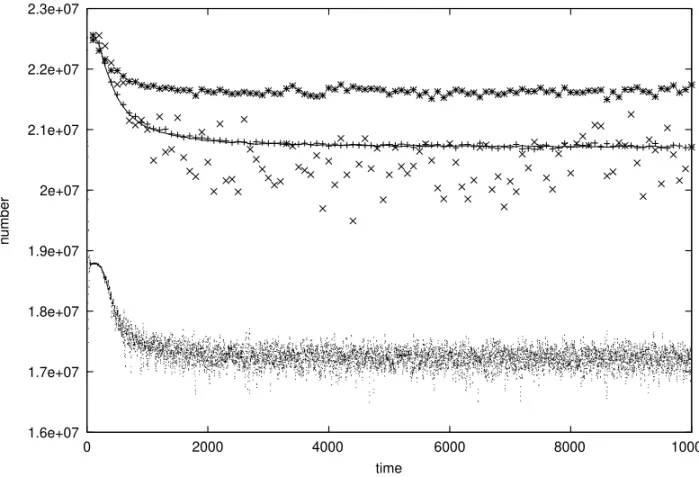
Fig. 3 – Comparison of populations, versus number of iterations or “years”, for (from below) SX, AP, MP. The highest data refer to a mixture of HA and MP withµ=4; nearly the same results are obtained forµ=3 and 5. The data for AS (line) overlap with those of MP (+), while AP(x) fluctuates around slightly lower values. For SX we show the sum of males and females. ThresholdT =9, 4 births per year and per female above minimum reproduction rate of 8, one mutation per string of 32 bits at birth,Nmax= 80 million is about four times larger than the actual populations.
nant diseases, SX lost out for the originally selected mutation rate (Redfield 1994) of 0.3. Increasing the mutation rate to 1 for both AS and SX, SX won (Stauffer 1999) over AS if the male mutation rate was the same as the female one, and AS won over SX when the male mutation rate was three or more times higher than the female one. Thus, as also ob-served in Nature, sometimes asexual and sometimes sexual reproduction is better.
A more realistic model, involving an explicit genome in the form of bit-strings, was more recently investigated by Örçal et al. (2000). It did not involve aging, however, since all bit positions were treated equally. Instead, Örçal et al. (2000) used the Jan et al. (2000) parameter µ defined such that only
individuals withµ and more mutations exchange genome. (The model is then closer to HA than to SX.) Healthy individuals without many mutations reproduce similarly to AS. Five different versions were studied, depending on the number of offspring and on whether individuals withµand more muta-tions mate only with each other or also with a wider population having less mutations. The simulation showed that in none of the five cases the sexual pop-ulation died out; in one case it won even completely and made the AS population extinct.
possible justification of sex comes only from intrin-sic genetic reasons, not from extrinintrin-sic or social rea-sons like parasites, changing environment, or child protection. On the other hand, there are also cases were asexual reproduction is better. With aging in-cluded to make the simulation more realistic, the next subsection will tell us a different story.
3.3.Comparison in Penna aging model
Most organisms age, and thus we should compare sexual and asexual reproduction in a model with ag-ing, where reproduction starts only after a certain age. The Penna model of section 2 is the only one for which we know of computer simulations for ag-ing and sex. The first comparisons of MP with SX in this model were published by Bernardes (1997). More recently, AS, AP, MP, HA and SX were simu-lated with it (Stauffer et al. 2000). We enlarge the range of possibilities by incorporating into it the Jan parameter (Jan et al. 2000)µsuch that organisms withµand more mutations try to find a partner with whom they exchange genome (HA and SX), while those with less thanµmutations use AP or MP. One counts only the mutations already set, up to the cur-rent age of each individual, to make the choice.
The simulated mixtures of reproduction were: MP-HA, MP-SX, AP-SX. In the first case, the final population depends non-monotonically onµ show-ing a maximum for intermediateµ, while in the two other mixtures the behaviour is monotonic making the mixtures less interesting. SinceT mutations kill an individual, we have 0 ≤ µ ≤ T, withµ = 0
describing pure HA andµ=T describing pure MP for the MP-HA mixture. Fig. 3 summarizes our main results.
We see that SX (the small dots in the lower half) is by far the worst, MP (+) and AS (line) give nearly identical results, AP (x) is slightly worse than AS, and finally a mixture of HA and MP (stars) with µ = 4 gives the best results. Why then do males
exist?
Some people claim men should eat less steaks and drink less alcohol. Taken to the extreme, we as-sume the males eat nothing and are so much smaller
than the females that they consume no space. Some animals followed this way of life long before us. Then their contribution to the Verhulst dying proba-bility(Nm+Nf)/Nmaxmentioned in section 2 be-comes negligible, and the dying probability is sim-plified toNf/Nmax. With this change, the popula-tion for SX roughly doubles, not surprisingly, and then SX is by far the best solution. The majority of the present authors insist that this result is an ar-tifact of the assumptions and is no way to regulate their lives. In the evolution of sex hundreds of mil-lion years ago it is difficult to imagine that together with the mutation towards SX, immediately also the male body size became much smaller and consumed much less food.
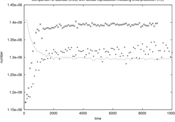
Perhaps male aggressiveness plays a useful role in protecting the children while reducing the male survival chances. Using the algorithm to be de-scribed in section 4 for testosterone as an explana-tion for the lower mortality of women compared to men, and female partner selection described later in this section, Fig. 4 shows that now SX is above MP or AS. This child protection is already an ef-fect outside the intrinsic genetic efef-fects discussed before. The following paragraphs discuss environ-mental effects which can also justify SX over AS, in agreement with reality.
Parasites have long been claimed to justify sex-ual reproduction, since the greater genetic variety of the offspring gives the parasites less chance to adapt to the host. An early computer simulation (Howard & Lively 1994) without aging already showed sex-ual reproduction to die out compared with asexsex-ual reproduction if no parasites are present (thus similar to Redfield 1994), while in the presence of parasites sex can give the better chance of survival (Howard & Lively 1994). Within the more realistic Penna model, including aging, the parasite problem was studied more recently by Sá Martins (2000) with the same result: Parasites justify sex.
1.15e+06 1.2e+06 1.25e+06 1.3e+06 1.35e+06 1.4e+06 1.45e+06
0 2000 4000 6000 8000 10000
n
umber
time
Comparison of asexual (lines) with sexual reproduction including child protection (+,x)
Fig. 4 – Comparison of populations, versus number of iterations, for SX with child protection (+,x), and AS (line). (For the data marked by x, females select only male partners with at most one active bad mutation.) Nmax= 5 million; otherwise parameters as in Fig. 3.
an individual can switch from MP to SX or back. The parasites are represented by bit-strings. Each female host has contact with 60 parasites, and if one parasite agrees in its bit-string with that of the fe-male, this host loses her ability to procreate. The parasite bit-string, on the other hand, is modified into the female bit-string if the parasite meets the same bit-string for the second time.
Starting with SX, the whole population changes to MP after a few hundred time steps, if no parasites are present. In the presence of parasites, however, starting with MP the whole population switches to SX in an even shorter time (Sá Martins 2000). Thus the well known greater variety of SX (Sá Martins & Moss de Oliveira 1998, Dasgupta 1997) compared to MP saves the sexual population from the attacks of parasites.
Both papers (Howard & Lively 1994, Sá
Mar-tins 2000) were motivated by observations of biol-ogist Lively and his collaborators on snails. They do not discuss if parasites already were plaguing the presumably much smaller organisms nearly 109
years ago when sex appeared.
0 10000 20000 30000 40000 50000 60000 70000
49900 49950 50000 50050 50100 50150 50200
n
umber
time
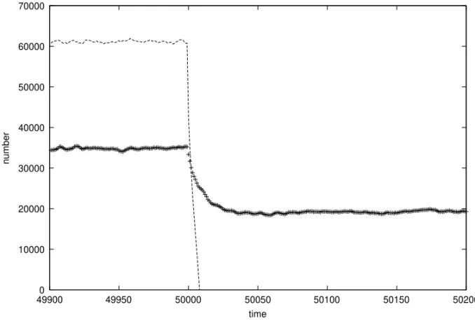
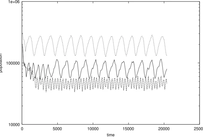
Fig. 5 – Comparison of MP (lines) with SX (crosses) population before and after a sudden change in the environment. For SX, the female birth rate of two was the same as for all MP individuals. (Nmax = 400000, T =3, d=5, R=10, one mutation per bit-string.)
chance to survive the catastrophe than MP.
Another reason why genomic exchange be-tween different individuals may be better than AS, AP or MP is partner selection (Redfield 1994, Stauf-fer et al. 1996). Let us simulate in the sexual Penna model first a birthrate of eight children per female and “year”; then we reduce the birth rate to four to account for males not getting pregnant; and in the third step we assume that the females select as part-ners only healthy males with few mutations. Some parameter region could be found, Fig. 6, where lection in step 3 gave a strong advantage over no se-lection (step 2), but this advantage was not enough to overcome the loss of half the births compared with step 1. With the parameters of Fig. 3 instead, the SX data would shift upward to 18.5 million if only males with at most one active mutation are selected. Thus, while the simpler models without aging gave clear intrinsic justifications for the existence of
males, the more realistic aging model required par-asites, catastrophes, or child protection for this pur-pose (partner selection may help somewhat) and in-trinsically slightly preferred a HA-MP mixture over haploid asexual cloning. It remains to be seen what SX simulations will give in other models (e.g. Onody 2000).
4. WHY WOMEN LIVE LONGER AND HAVE MENOPAUSE?
Men may be useless according to section 3.3, but why do they live shorter than women, in the devel-oped countries of the 20th century?
10000 100000 1e+06
0 5000 10000 15000 20000 25000
population
time
Fig. 6 – Can partner selection overcome the loss of half the births? The top data show step 1, the bottom data step 2, and the middle data step 3 (see text): Selection helps, but not enough.
roughly the same mutations from the parents; for the same reason, women are not killed by mutations after menopause (see below), in contrast to Pacific Salmon (Moss de Oliveira et al. 1999a, Penna et al. 1995). Somatic mutations, which are not inher-ited and not given on to the offspring, reduce the male mortality compared to the female one if the rate of somatic mutations is higher for males than for females (Moss de Oliveira et al. 1996). Alter-natively, females could be just more resistant than males against diseases (Penna & Wolf 1997). Mam-malian females have two X chromosomes, while the males have one X and one Y chromosome such that all X mutations are dominant (Schneider et al. 1998). Except at old age, these last three assump-tions all lead to higher male than female mortalities, as in reality (Fig. 1), and where reviewed in our book (Moss de Oliveira et al. 1999a).
A more recent idea was suggested to us by
the medical researcher Klotz and is related to male lifestyle (steaks and alcohol) caused by testosterone (Klotz 1998, Klotz & Hurrelmann 1998, Baulieu 1999). This hormone causes higher male aggressiv-ity leading to death, as well as more arteriosclerosis later in life. These bad effects were perhaps coun-terbalanced earlier in human evolution by helping the males to defend their families against predators or fellow men. This child protection by males can in some other form also occur in other animals. Us-ing this child protection assumption together with sexual selection as described below, the above SX results in Fig. 4 were produced. And for today’s hu-mans, the testosterone parameters of this child pro-tection model could be chosen such that the male mortality is about twice as high as the female mor-tality, except at old age, in agreement with reality (Stauffer & Klotz 2000, Stauffer 2000).
between the mortalities of men and women is a com-bination of genetic and social effects, as is shown by the variation from country to country within Europe (Gjonça et al. 1999). The XX-XY chromosome hy-pothesis (Schneider et al. 1998) is supported by the observation (Paevskii 1985) that male birds usually live longer than the females: For birds, the females have two different and the males have two identical chromosomes, opposite to mammals.
(Technical remark: To simulate the effects of male testosterone level in Fig. 4, the Verhulst dy-ing probability was increased, for males only, by an amount proportional to the age-dependent tes-tosterone levelk(a)(Stauffer & Klotz 2000, Stauf-fer 2000). On the other hand, the probability of babies to survive was multiplied by a factor min(const·k(a),2) such that a too low testosterone level of the father causes his babies to be killed by others. The functionk(a)evolved to an optimum shape through small heritable mutations ink(a).)
Menopause for women means an abrupt ceas-ing of their reproductive function, while for men, andropause is a rather smooth decay with age. Sim-ilar effects exist for the other mammals (though per-haps under different names, which we ignore here). For Pacific Salmon, life ends for males and females shortly after the end of reproduction of both (Penna et al. 1995); why does the same effects not occur for women?
Pure genetic reasons (Stauffer et al. 1996) in the unmodified Penna model, without child care, al-ready allow women to survive menopause. Concep-tion decides randomly whether the new baby is a boy or a girl, and the genome is the same apart from the difference in X and Y chromosomes. Thus if all bits above reproductive age would be set equal to one for women (as for Pacific Salmon), the men would also die at that same age of menopause. To kill the women earlier than men, mother Nature would need a longevity gene in the Y chromosome, which in re-ality contains little genetic information. In this way, female survival after menopause is consistent with the mutation-accumulation hypothesis in the Penna model.
This consistency does not yet explain why menopause evolved. The only simulation we are aware of explaining menopause (Moss de Oliveira et al. 1999b) introduces two new assumptions into the Penna model: a risk of dying at birth for the mother which increases with the number of active muta-tions and thus with age; and child care in the sense that young children die if their mother dies. Then the maximum age for reproduction was allowed to emerge from the simulation, instead of being put in fixed at the beginning, by assuming it to be hered-itary apart from small mutations up or down. As a result, the distribution of the maximum age of repro-duction peaked at about 15 “years” whereas without child care its maximum was at 32 years, at the oldest possible bit position.
5. OTHER ASPECTS
Geneticist S. Cebrat (priv. comm.) has criticized our crossover method for the sexual Penna model as published in Moss de Oliveira et al. (1999a). Since we split the bit strings at some randomly selected position and then combine the first part of one bit-string with the second part of the other bit-bit-string, and since bit positions correspond to individual age, we produce correlations for the mutations in con-secutive ages. In real DNA, the genes are not stored consecutively in the order in which they become ac-tive during life. Thus it is better to select randomly one subset of bits from one bit-string, and the other bits from the complimentary bit-string. Simulations indicate no clear difference, Fig. 7.
Overfishing (Moss de Oliveira et al. 1995, Penna et al. 2000) and the inheritance of longevity (de Oliveira et al. 1998) were simulated using the asexual version of the Penna model.
0.001 0.01 0.1 1 10
0 5 10 15 20
mor
tality function
age
Fig. 7 – Comparison of traditional ordered crossover (x, squares) with better random crossover (+, stars) showing little difference. The Verhulst deaths appear at all ages (+, x) or only at birth (stars, squares).
Partridge and Barton review (Partridge & Barton 1993). There they proposed a constraint for the sur-vival rates from babies to juvenilesJ and juveniles to adultsAasJ+A4=1. Because it has only two
parameters and three ages, the exponential increase of mortalities cannot be observed. Some attempts of implementing antagonistic effects on bit-string models have been done. Bernardes imposed an ex-tra deleterious mutation at advanced ages for a frac-tion of the populafrac-tion with higher reproducfrac-tion rates (Bernardes 1996). Sousa and Moss de Oliveira, in a more detailed study, have shown that the combined action of mutation accumulation and antagonistic pleiotropy at defined ages can extend the lifespan of a population (in preparation). Sousa and Penna have introduced a different strategy, where both sides of the antagonism are present: good (bad) mutations at earlier (later) ages (in preparation). The minimum
age at reproduction is allowed to vary. The later the individual reaches the sexual maturity, the more fer-tile it is. There is a clear compromise to postpone the maturity (and consequently to decrease the inte-grated fertility) against to be more exposed to death by competition or action of bad mutations. Pre-liminary results suggest that except for unrealistic handicaps on the fertility for later maturity, natural selection drives the populaton to earliest maturity (see also Medeiros et al. 2000).
6. CONCLUSIONS AND PERSPECTIVES
hap-loid genomes. We speculate that from this asexual way, mother Nature may have evolved via apomictic and/or meiotic parthenogenesis towards hermaphro-ditism, and only later separated the population into males and females because of external or social rea-sons, as simulated. Finally, menopause appeared because of the need for child care by the mother and the risks for her associated with giving birth later in life. For practical applications, simulations sug-gested not to catch young fish, or young and old lobsters, in order to maximize the catch (Moss de Oliveira et al. 1995, Penna et al. 2000).
7. ACKNOWLEDGMENT
We are indebted to the Brazilian agencies CAPES, CNPq and FAPERJ for partial financial support.
RESUMO
A versão sexual do modelo de envelhecimento biológico de Penna, simulada desde 1996, é comparada aqui com formas alternativas de reprodução bem como com mo-delos que não envolvem envelhecimento. Em particular, queremos verificar como formas sexuais de vida pode-riam ter evoluído e predominado sobre formas assexuais há centenas de milhões de anos. Este modelo computa-cional baseia-se na teoria do envelhecimento por acumu-lação de mutações, usando ’bits-strings’ para representar o genoma. Sua dinâmica de populações é estudada por métodos de Monte Carlo.
Palavras-chave: partenogênese, genoma, menopausa, testosterona, simulação Monte Carlo.
REFERENCES
Azbel MYa. 1994. Universal biological scaling and
mortality.Proc Natl Acad Sci USA91:12453-12457.
Bak P.1997. How Nature Works: the Science of
Self-Organized Criticality, Oxford University Press.
Baulieu EE.1999. Le vieillissement est-il soluble dans
les hormones? La Recherche322:72-74.
Bernardes AT. 1995. Mutational meltdown in large
sexual populations.J PhysiqueI5:1501-1515.
Bernardes AT.1996. Strategies for reproduction and
aging.Ann Physik5: 539-550.
Bernardes AT.1997. Can males contribute to the genetic
improvement of the species? J Stat Phys86: 431-439.
Darwin C.1859.On the Origin of Species by Means of
Natural Selection, Murray, London.
Dasgupta S.1997. Genetic crossover vs. cloning by
computer simulation.Int J Mod PhysC8: 605-608.
de Oliveira PMC.1991.Computing Boolean Statistical
Models, World Scientific, Singapore/ London/ New York.
de Oliveira PMC.2000. Why do evolutionary systems
stick to the edge of chaos.Theory in Biosci: in press.
de Oliveira PMC, Moss de Oliveira SM, Bernardes
AT & Stauffer D.1998.Lancet352:911-912.
Excoffier L.1997. Ce que nous dit la genealogie des
genes.La Recherche302:82-84.
Gjonça A, Tomassini C & Vaupel JW.1999. Pourqoi
les femmes survivent aux hommes? La Recherche 322:96-99.
Holbrook NJ, Martin GR & Lockshin RA.1996.
Cel-lular Aging and Death, Wiley-Liss, New York.
Howard RS & Lively CM.1994. Parasitism, mutation
accumulation and the maintenance of sex. Nature 367:554-557 and368:358 (Erratum).
Jacquard A.1978.Éloge de la Différence: la Génétique
et les Hommes, Éditions du Seuil, Paris.
Jan N, Moseley L & Stauffer D.2000. A hypothesis
for the evolution of sex.Theory in Biosci119: 166-168.
Kauffman SA.1993. Origins of Order:
Self-Organi-zation and Selection in Evolution, Oxford University Press, New York.
Kauffman SA.1995. At home in the Universe, Oxford
University Press, New York.
Klotz T.1998.Der frühe Tod des starken Geschlechts,
Cuvillier, Göttingen.
Klotz T & Hurrelmann K.1998. Adapting the health
Lynch M & Gabriel W.1990. Mutation load and the survival of small populations. Evolution44: 1725-1737.
Medeiros G, Idiart MA & de Almeida RMC.2000.
Selection experiments in the Penna model for biolog-ical aging.Int J Mod PhysC11:No. 7.
Moss de Oliveira S, Penna TJP & Stauffer D.1995.
Simulating the vanishing of northern cod fish. Phys-icaA215:298-304.
Moss de Oliveira S, de Oliveira PMC & Stauffer D. 1996. Aging with sexual and asexual reproduction: Monte Carlo simulations of mutation accumulation. Braz J Phys26:626-630.
Moss de Oliveira S, de Oliveira PMC & Stauffer D.1999a. Evolution, Money, War and Computers, Teubner, Leipzig.
Moss de Oliveira S, Bernardes AT & Sá Martins JS.1999b. Self-organisation of female menopause in populations with child care and reproductive risk. Eur Phys JB7:501-504.
Onody RN.2000. The Heumann-Hötzel Model revisited.
Talk O-24 at FACS 2000, Maceió, Brazil.
Örçal B, Tüzel E, Sevim V, Jan N & Erzan A.2000.
Testing a hypothesis for the evolution of sex. Int J Mod PhysC11:973-986; and also DeCoste C & Jan N, priv. comm.
Paevskii VA.1985. Demography of Birds(in Russian),
Nauka, Moscow.
Pamilo P, Nei M & Li WH. 1987. Accumulation of
mutations in sexual and asexual populations. Genet Res, Camb49:135-146.
Partridge L & Barton NH.1993. Optimality, mutation
and the evolution of aging.Nature362:305-311.
Penna TJP.1995. A bit-string model for biological aging.
J Stat Phys78:1629-1633.
Penna TJP & Moss de Oliveira S.1995. Exact results
of the bit-string model for catastrophic senescence. J PhysiqueI5: 1697-1703.
Penna TJP & Stauffer D.1996. Bit-string aging model
and German population.Zeits PhysB101:469-470.
Penna TJP & Wolf D.1997. Computer simulation of
the difference between male and female death rates. Theory in Biosc116:118-124.
Penna TJP, Moss de Oliveira S & Stauffer D.1995.
Mutation accumulation and the catastrophic senes-cence of the Pacific salmon.Phys RevE52: R3309-R3312.
Penna TJP, Racco A & Sousa AO. 2000. Can
mi-croscopic models for age-structured populations con-tribute to Ecology? Talk IT-11 at FACS 2000, Ma-ceió, Brazil (to appear inPhysica A).
Redfield RJ.1994. Male mutations and the cost of sex
for males.Nature369:145-147.
Rose MR.1991.Evolutionary Biology of Aging, Oxford
University Press, New York.
Sá Martins JS.2000. Simulated coevolution in a
mu-tating ecology.Phys RevE61:2212-2215.
Sá Martins JS & Moss de Oliveira S.1998. Why sex
– Monte Carlo simulations of survival after catastro-phes.Int J Mod PhysC9:421-432.
Schneider J, Cebrat S & Stauffer D.1998. Why
do women live longer than men? A Monte Carlo Simulation of Penna-type models with X and Y cro-mossomes. Int J Mod PhysC9:721-725.
Schrödinger E.1944. What is Life?, Cambridge
Uni-versity Press, Cambridge.
Sousa AO& Moss de Oliveira S.1999. High
repro-duction rate versus sexual fidelity.Eur Phys JB10:
781-785.
Stauffer D.1994. Monte Carlo simulations of
biologi-cal aging.Braz J Phys24:900-906.
Stauffer D.1999. Why care about sex? Some Monte
Carlo justification.PhysicaA273:132-139.
Stauffer D. 2000. Self-organisation of testosterone
level in the Penna-Klotz aging model.Theory in Bio-sciences, in press.
Stauffer D & Aharony A.1994.Introduction to
Per-colation Theory, Taylor and Francis, London.
Stauffer D & Klotz T.2000. The mathematical point
in-fluence of testosterone in an aging simulation model and its consequences for prevention. Submitted to The Aging Male.
Stauffer D, de Oliveira PMC, Moss de Oliveira S
& Zorzenon dos Santos RM.1996. Monte Carlo
simulations of sexual reproduction. PhysicaA231:
504-514.
Stauffer D, Sá Martins JS & Moss de Oliveira S. 2000. On the uselessness of men – Comparison of sexual and asexual reproduction. Int J Mod PhysC
11:No. 7.
Vaupel JW, Carey JR, Christensen K, Johnson TE, Yashin AI, Holm NV, Iachine IA, Kanisto V, Khazaeli AA, Liedo P, Longo VD, Zeng Y,
Manton KG & Curtsinger JW. 1998.
Biode-mography of longevity. Science280:855-860.
Wachter KW & Finch CE.1997.Between Zeus and the
Salmon. The Biodemography of Longevity, National Academy Press, Washington DC.
Wilson KG. 1971. Renormalization group and
crit-ical phenomena I. Renormalization group and the Kadanoff scaling picture.Phys RevB4:3174-3183.
Wilson KG.1979. Problems in physics with many scales
of length.Sci Am241:140-157.
Wilson KG & Kogut J.1974. The renormalization