Greenhouse Gases Emissions and
Economic Performance of Livestock,
an Environmental Input-Output Analysis
1Luiz Carlos de Santana Ribeiro
2, Eder Johnson de Area Leão
3and Lúcio Flávio da Silva Freitas
4Abstract: In the last three decades, the developing countries have sharply increased its contribution to global warming. From 2005 to 2012, Brazil has reduced its total emissions in 12% due to deforestation control. In the same period, the total GHG emissions excluding land-use change and forestry have increased 18% (WRI, 2014), while per capita GPD has raised 17%. The Brazilian climate policy must go beyond the deforestation control to avoid an unsustainable pattern of development. Since the mitigation effort bears heavily on primary activities, one must ask: how important are those sectors for Brazilian economy? And how their emissions are connected to other sectors along the productive chain? Specifically, this paper aims to calculate the GHG emissions multipliers of the Brazilian economy in 2009 and associate these results with the employment and income multipliers, particularly of the Agriculture sector. The ‘field of influence’ method (SONIS and HEWINGS, 1992) is applied to calculate the intersectorial relations in terms of input linkages and GHG emissions.
Key-words: input-output, GHG emissions, agriculture, Brazilian economy.
Resumo: Nas últimas três décadas, os países em desenvolvimento aumentaram significativamente a sua contribuição para o aquecimento global. O Brasil, entre 2005 e 2010, reduziu suas emissões totais em 12%, devido ao controle do desmatamento. No mesmo período, as emissões totais de GEE, excluindo mudanças no uso da terra e florestas, aumentaram 18% (WRI, 2014), enquanto o PIB per capita aumentou 17%. A política climática brasileira deve ir além do controle do desmatamento para evitar um padrão insustentável de desenvolvimento. As principais medidas para o controle das emissões são aplicadas às atividades primárias, assim, cabe perguntar: qual a importância dessas atividades para a economia brasileira? E como as suas emissões estão ligadas às emissões de outras atividades ao longo da
1. Data de submissão: 12 de junho de 2016. Data de aceite: 11 de setembro de 2017.
2. Universidade Federal de Sergipe. São Cristóvão-SE, Brasil. E-mail: [email protected] 3. Instituto Federal de Educação do Maranhão. Bacabal-MA, Brasil. E-mail: [email protected].
O autor agradece ao suporte financeiro da Fundação de Amparo e Pesquisa do Estado da Bahia – Fapesb.
1. Introduction
In the last three decades the developing countries have sharply increased its contribution to global warming. In the near future they will become the major part of world GHG emissions (GOLDEMBERG and GUARDABASSI, 2012). Because of accumulated emissions, the developed economies should take the leadership on fighting global warming. Nevertheless, the developing world should find the cleanest route to affluence.
For instance, from 2005 to 2012, Brazil has reduced its total emissions in 12% due to deforestation control. In the same period, the total GHG emissions excluding land-use change and forestry have increased 18% (WRI, 2014), while per capita GPD has raised 17%. The Brazilian climate policy must go beyond the deforestation control to avoid an unsustainable pattern of development. Otherwise, in the long run the Brazilian emissions could reach a similar level of nowadays developed countries.
In fact, the Brazilian Intended Nationally Determined Contributions (INDCs) wants more. It aims to “zero illegal deforestation by 2030 and compensating for greenhouse gas emissions from legal suppression of vegetation by 2030” (BRAZIL, 2015, p. 7). And also to increase the use of renewable energy sources, promoting the restoration and reforestation of 12 million hectares of degraded land (BRAZIL, 2015) and reinforcing the Low Carbon Agriculture Plan. Deforestation is usually connected to agricultural activities, mainly cattle production (BUSTAMANTE et al., 2012). Altogether INDCs is supposed to reduce the Brazilian GHG emissions by 43% below 2005 levels in 2030.
Since the mitigation effort bears heavily on primary activities, one must ask: how important are those sectors for Brazilian economy? And how their emissions are connected to other sectors along the productive chain? Worldwide the main source of GHG is fossil fuel consumption (IPCC, 2001). However, in the primary sectors, emissions are mainly the result of biotic processes, as enteric fermentation and changes in land use, especially deforestation (MOSIER et al., 1998; JANZEN, 2004; SMITH and CONEN, 2004).
The direct and indirect emissions throughout the productive chain may be assessed by using extended input-output models that incorporate environmental aspects. Using this framework, Young (2011) has demonstrated that the most Brazilian dynamic sectors, in terms of jobs, wages and GDP, are the less pollutant ones, regarding to the potential pollution indices from Industrial Pollution Projection System (HETTIGE et al., 1994). Montoya et al. (2016) estimated the requirement of fossil fuel and the emissions’ multipliers of economic activities. The service sector had an important contribution to GHG from fossil fuel consumption. Also Lenzen et al. (2013) decomposed the Brazilian CO2 emissions from 1970 to 2005. The per capita GDP is the most important driver of emissions and the cattle production is the economic activity that emits more.
The international literature presents many studies about the intensity of CO2 or GHG emissions in economic sectors for different countries/regions from an environmental input-output framework. Studies by Carvalho et al. (2013), Rhee and Chung (2006) and Su et al. (2013), based on international trade’s perspective, evaluated CO2 emissions of Minas Gerais (Brazilian state), between Korea and Japan and China, respectively. Yamakawa and Peters (2011), Butnar and
O método de “campo de influência” (SONIS and HEWINGS, 1992) é aplicado para calcular as relações intersetoriais e as emissões de GEE.
Palavras-chaves: insumo-produto, emissões de GEE, agropecuária, economia brasileira.
JEL Classification: Q54, Q56, Q10.
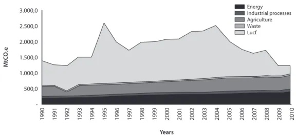
Figure 1. Greenhouse gas emissions in Brazil, 1990 to 2010
Energy
Industrial processes Agriculture Waste Lucf 3.000,0
Years
1990 1991 1992 1993 1994 1995 1996 1997 1998 1999 2000 2001 2002 2003 2004 2005 2006 2007 2008 2009 2010 2.500,0
2.000,0
1.500,0
MtC
O2
e
1.000,0
500,0
-a) The gases listed in these estimates were carbon dioxide (CO2), methane (CH4), nitrous oxide (N2O), hydrofluorocarbons (HFCs), perfluocarbons
(FC’s) and sulfur hexafluoride (SF6). Emissions in CO2eq.
b) LUCF is the Land Use Change and Forestry.
c) The Energy sector comprises emissions from fossil fuel combustion related to the oil, gas and coal production. In the industrial processes, emissions arise from the production processes themselves, exclusively those resulting from fuel combustion, which is accounted for in the energy category. d) In agriculture, emissions from enteric fermentation of herds, rice cultivation, animal waste management, agricultural land and burning of agricultural residues were considered.
e) In LUCF the balance between removals and emissions between different land uses, in addition to liming and biomass burning (MCTI, 2013).
Source: MCTI (2013).
Llop (2011), Silva and Perobelli (2012) and Brizga et al. (2014) used the structural decomposition analysis (SDA) to evaluate CO2 or GHG emissions in Norway, Spain, Brazil and Baltic States, respectively. Cristóbal (2010, 2012), Hristu-Varsakelis et al. (2010) and Hristu-Varsakelis
et al. (2012) used an environmental input-output linear programming model to minimize GHG emissions subject to environmental and economic constraints.
All those studies have used input-output models that somehow cover the intensities of emissions. None of them, however, has been concerned with specifically analyzing the role of the agriculture/livestock sector as an important generator of GHG emissions and its relationship with its economic performance and linkages effects.
Specifically, this paper aims to calculate the GHG emissions multipliers of the Brazilian economy in 2009 and associate these results with the employment and income multipliers, particularly of the Agriculture and Livestock sectors. The “field of influence” method (SONIS and HEWINGS, 1992) is applied to calculate the intersectorial relations in terms of input-output linkages and GHG emissions. In this regard, data from Nereus (GUILHOTO and SESSO FILHO, 2005, 2010)
were used to construct an environmental input-output model for Brazil. To achieve the proposed objectives, Section 2 presents data about the GHG Brazilian emissions. Section 3 presents the input–output (IO) model incorporating GHG emissions and some IO indicators. Section 4 describes the database. Section 5 presents and discusses the empirical results and Section 6 presents the conclusions.
2. GHG Brazilian emissions
Two trends have been quite prominent in the Brazilian emissions: i) the change in total due to LUCF, with progressive decrease since its peak in 2004, and ii) the continued increase in emissions by other sour-ces, notably agriculture and energy generation. The Brazilian INDCs is supposed to reduce total emissions and to change its main sources. While deforestation, agricultural and forestry sectors would reduce the total GHG emissions, the other sources together are allowed to increase in 21% their emissions.
Agriculture and Livestock have emitted 437 MtCO2eq in 2010, that is, 35% of total emissions. In this sector, methane from enteric fermentation in ruminants accounted for 56.2% of emissions, and agricultural soils by other 35.2%, mainly by animal manure on pasture and nitrogen fertilizer use. Animal waste management, especially with respect to herds raised in intensive confinement, which favors anaerobic decomposition of waste, has emitted 4.9%; the cultivation of rice, 2%; and burning waste from sugarcane and cotton, 1.5%. Since 1990 emissions growth in agriculture has been of 43%.
Beef cattle totaled almost 90% of the methane from enteric fermentation in 2005 (MCTI, 2010). The prospect in this segment is of an emission increase in the mid-term. There is an increasing global demand for beef. Furthermore, Brazil is the second largest exporter, after Australia. Currently, domestic demand represents 84% of production and per capita consumption is 40 kg/year, surpassed only by Argentina, 51 kg. Slaughter grew at 5.1% per year between 2000 and 2011 (LOYOLA, 2013).
According to IBGE (2009), Brazil has 190 million head cattle herd in 2009, being the second largest slaughterer country, only behind China. Ranching occupies 199,000 hectares, the largest area among all agricultural activities in Brazil. Livestock market also has lower employment generation per area, one job per 500 hectares. There is also a high informality in the sector. In 2006, the livestock market generated only 440 thousand formal jobs, 43% of which were generated in the Southeast, a region that corresponds to only 19% of the Brazilian cattle.
Net emissions of LUCF were 279 MtCO2eq, or 22% of 1,246 Mt emitted in 2010. Almost all of these emissions have been caused by deforestation, except 10 Mt that was due to the application of Calcium (liming). The main gas was carbon dioxide (90%). Among the Brazilian biomes, the Amazon and the
Cerrado together accounted for 93% of net emissions of LUCF (MCTI, 2013).
According to Houghton (2005) the emissions from tropical deforestation are determined by two factors: i) rates of land-use change (including harvest of wood and other forms of management) and ii) per hectare changes in carbon stocks following deforestation (or harvest). The amount of carbon held in trees is 20-50 times higher in forests than in cleared lands, and changes in carbon stocks vary with the type of land use (for example, conversion of forests to croplands or pastures), with the type of ecosystem (tropical moist or tropical dry forest), and with the tropical region (Asia, America, or Africa).
In the past two decades, Brazil has been the world leader in tropical deforestation, clearing an average of 19,500 km2/year from 1996 to 2005. This forest conversion to pasture and farmland released from0.7 to 1.4 GtCO2eq per year to the atmosphere. According to FAO (2010), the highest rates of deforestation (in 106 ha/year during the 1990s) occurred in Brazil.
The main causes of deforestation in Brazil, specifically in the Amazon, are its exploitation for timber and agriculture (NEPSTAD et al., 2001; MARGULIS, 2003; FEARNSIDE, 2005; RIVERO et al., 2009). Even with the supervision of the federal government, there is an illegal large-scale harvesting of timber, especially the most profitable species (mahogany and ipe).
A reduction in deforestation has been achieved after 2004, when The Action Plan for Prevention and Control of the Legal Amazon Deforestation (PPCDAM) and analogue plans for Cerrado and Caatinga regions were released. Through such measures, the Brazilian government took the responsibility to control deforestation and reduce it to a minimum rate by the year 2020 (MMA, 2013). In the Amazon biome the annual rate dropped from 27,772 km² in 2004 to 6,418 km² in 2011. In 2012, the figure of 4,571 km² was the lowest ever recorded by the Project of Deforestation Monitoring in the Legal Amazon, and in 2013, 5,891 km² have been deforested (PRODES/INPE, 2014). In Cerrado, the drop was from the average of 14,179 km² in the period 2002-2008 to the average of 6,469 km² in 2009-2010 (MCTI, 2013). In 2010, the GHG annual emissions were 65% lower than those registered in 1990.
that crops have advanced faster than livestock, and it also expands to states that have a well-structured agribusiness such as Mato Grosso and Tocantins. In the 1990s, according to Costa (2000), tax incentives from the federal government for ranchers through Finam (Amazon Fund), rural credit and FNO (Constitutional Fund for the development of the North region) may have encouraged deforestation in the Amazon.
Between 2004 and 2010 the Brazilian economy registered strong growth in production, more than 4% per year. The decoupling of LUCF emissions from the economic cycle reveals that the country had an advantage to reduce its emissions. It is not the same to other emerging countries where GHG releases are most associated with energy generation, such as China or Russia.
3. The input-output model
incorporating emissions
The input-output model traces the trade between industries and the final demand of the economy in an integrate perspective. More specifically, according to Leontief (1941): “An attempt to apply the economic theory of general equilibrium – or better, general interdependence – to an empirical study of inter-relations among the different parts of a national economy as revealed through covariations of prices, outputs, investments and incomes” (p. 3). This model may be represented by the following system of matrix equations:
x
=
Ax
+
F
(1)
x
= (
I
–
A
)
-1f
(2)
In which x and f are respectively the total output and final demand; A = [aij] is the Technological Matrix
defined as quantity of intermediate input used by sector i to produce an output unit of production sector
j (in monetary terms), for i, j = 1, …, n; and L = (I – A)-1 is the Leontief Inverse Matrix.
To incorporate emissions associated with the production of inter-sector activities, according to Miller and Blair (2009), we consider a matrix of direct emissions coefficients Ep = [ep
kj], wherein each element indicates
the amount of pollutants of the type k, generated per unit of production of industry j. Therefore, the level of
emissions associated with the vector of total output can be expressed as:
x
p=
E
px
(3)
In which xp is a vector that represents the level of
emissions per economic activity. Combining equations 2 and 3, there is:
x
p=
E
p(
I
–
A
)
-1or
x
p= [
E
p⋅
L
]
⋅
f
(4)
The result of the multiplication [Ep⋅L] represents
a matrix of total coefficients of environmental impact, that is, the elements of this matrix represent the total emissions impact generated per unit of final demand.
There are several methods of analysis that can be calculated from the input-output tables. For the present article, we calculate the multipliers for emissions, employment and income. Furthermore, to measure the linkages effects, it is also calculated the traditional field of influence and the field of influence that incorporates emissions.
3.1. Input-output indicators
Input-output multipliers are overall used to evaluate the impact of exogenous changes on the output, income, employment, value added, among other variables. The simple output multiplier of sector
j (Mp
j) can be defined as the total required emissions
from all sectors, to meet the variation in a monetary unit of the total demand of sector j (MILLER and BLAIR, 2009), and can be expressed by:
M
je l
p kj p
ij i
n
1
$
=
=
/
(5)
Wherein lij are the elements of the Leontief Inverse
Matrix. It is important to highlight that the simple multiplier is calculated from a model with household exogenous. The employment multiplier is defined (Mej) as follows:
Me
jv L
iji n
1
$
=
=
t
6 @
/
(6)
In order to identify the strongest linkages that may cause greater impacts on the Brazilian economy, the field of influence developed by Sonis and Hewings (1992) is presented. From it, it is possible to view the sectors that exerted greatest influence, from their intersectoral relationships, on the rest of the economy. To evaluate the impact of these variations on each element of the Technological Matrix (A), a small change (ε)5 must occur, on each a
ij isolatedly, (i.e.), ∆A is a matrix
C = |εij|. If the change occurs in location (i1, j1) i.e.:
if i
i
j
j
if i
i
j
j
0
and
and
ij 1 1 1 1!
!
ε
ε
=
=
=
*
(7)
In this case, a variation of magnitude ∆A in the coefficients of Matrix A results in a new Technological Matrix: A* = A + ∆A. Accordingly, Leontief Inverse Matrix may be rewritten as: L* = (I – A – ∆A)-1. The field of influence (F) of each coefficient is approximately equal to:
*
F
ijL
L
ij
ε
ε
=
−
^ h
(8)
The total influence of each technical coefficient of the input-output matrix is given by equation (9). The higher the Sij, the larger the field of influence of
coefficient aij on the productive structure.
S
ijf
kl ij l n k n 2 1 1ε
=
= = ^ h 6 @/
/
(9)
To incorporate the emissions, a new matrix G is used, in which G = Ep⋅ (I – A)-1 and G* = Ep⋅ (I – A –
∆A)-1, therefore equation (8) may be rewritten as:
*
F
ijG
G
ij
ε
ε
=
−
^ h
(10)
To calculate the new field of influence that incorporates the direct coefficients of GHG emissions, it is simply necessary to use the result obtained by equation (10) in equation (9).
The input-output matrix used in this paper was taken from the Nereus database (GUILHOTO and SESSO FILHO, 2005, 2010). This database was built from official information of national accounts, and comprises a set of annual input-output tables for the period of 2000-2009, at the level of 56 sectors of economic activity. The data from GHG emissions was
5. ε = 0.001.
taken from the Brazilian inventory of GHG emissions, compiled by the Ministry of Science, Technology and Innovation (MCTI, 2013).6
The intermediate emissions were taken according to intermediate consumption share on total consumption. The emissions from fossil fuel consumption were distributed amongst the economic sectors according to their share on intermediate consumption, by type of fuel, on monetary values.7 The same way, the emissions from production processes were distributed according to the sectorial share on intermediate production, by type of process that release GHG.
4. Results and discussion
According to the World Bank data, in 2009 Brazil was ranked as the world’s tenth largest economy in terms of GDP. In the same year, according to World Resources Institute, the country emitted 870.74 million tCO2eq. excluding Land-use Change and Forestry (LUCF), accounting for 2.1% of global emissions. Other emerging countries, such as China, India and Russia, emitted more GHG than Brazil. In the same year, their shares on global emissions were, respectively, 22%, 6% and 5% (WRI, 2014). Figure 2 represents the Brazilian GHG emissions per major economic sectors.
Agriculture and livestock, in 2009, accounted for 47% of total GHG emissions in Brazil, followed by energy sector. This is due to enteric fermentation of livestock, animal waste management, agricultural soils, rice cultivation, burning of agricultural wastes (MOSIER
et al., 1998; SMITH and CONEN, 2004; JANZEN, 2004; MCT, 2010). Is the environmental cost generated by agriculture and livestock reversed in economic returns through the generation of employment and income, for instance? To answer this question, the results of the emissions multiplier reported in Table 1 have been confronted with the results of traditional employment and income multipliers.
6. Only CO2, N2O, and CH4 were considered. These gases
are more than 95% of Brazilian total CO2 equivalent
emissions.
Figure 2. Percentage of GHG Brazilian direct emissions, excluding LUCF – 2009
Energy; 42%
Industrial processes; 5% Agriculture; 47%
Waste; 5% Bunker fuels; 2%
Source: WRI (2014).
Table 1. Multipliers of GHG emissions, employment and income – 2009
Sectors GHG
(tCO2eq)
GVP (R$ 1,00)
Production Multiplier Traditional multipliers
GHG/GVP (direct effect)
Indirect effect
Total
effect Empl. Income 1. Agriculture, forestry, extractive 26.082.858 176.093.00 0,15 0,13 0,28 77 0,23
2. Livestock and fishing 413.971.696 100.354.000 4,13 0,48 4,61 70 0,31
3. Oil and natural gas 19.362.452 81.614.000 0,24 0,15 0,38 12 0,26
4. Iron ore 3.530.316 29.516.00 0,12 0,14 0,26 9 0,18
5. Other mining and quarrying 21.581.181 19.494.00 1,11 0,21 1,32 21 0,27
6. Food and beverage 5.404.611 358.919.000 0,02 1,01 1,02 44 0,30
7. Smoking products 10.909 11.408.000 0,00 0,19 0,19 41 0,26
8. Textiles 1.311.124 40.363.000 0,03 0,14 0,17 42 0,29
9. Vestment goods and acessories 45.742 41.550.000 0,00 0,08 0,08 64 0,35 10. Leather goods and footwear 38.422 24.239.000 0,00 0,17 0,17 44 0,40 11. Wood products – excluding furniture 166.161 19.285.000 0,01 0,12 0,13 46 0,34 12. Pulp and paper products 4.488.480 45.049.000 0,10 0,17 0,27 23 0,29 13. Newspapers, magazines, discs 27.108 38.675.000 0,00 0,08 0,08 20 0,29 14. Oil refining and coke 32.650.376 150.105.000 0,22 0,23 0,45 9 0,17
15. Alcohol 2.918.339 22.444.000 0,13 0,23 0,36 45 0,25
16. Chemicals 12.671.257 64.447.000 0,20 0,24 0,44 12 0,22
17. Manufacture of resin and elastomers 1.006.111 21.566.000 0,05 0,19 0,24 11 0,22 18. Pharmaceutical products 700.775 39.496.000 0,02 0,10 0,12 13 0,27
19. Agrochemicals 277.844 16.735.000 0,02 0,15 0,17 15 0,27
20. Perfumes, hygiene and cleaning 21.390 26.960.000 0,00 0,19 0,19 20 0,25 21. Paints, varnishes, enamels and lacquers 1.859.994 12.358.000 0,15 0,17 0,32 13 0,26 22. Diverse chemical products and mixtures 129.116 14.787.000 0,01 0,14 0,15 17 0,27 23. Rubber and plastic goods 569.606 60.196.000 0,01 0,13 0,14 17 0,28
24. Cement 28.402.670 11.889.000 2,39 0,27 2,66 13 0,23
25. Other products of non-metallic minerals 12.084.047 40.368.000 0,30 0,32 0,62 26 0,31
26. Manufacture of steel and derivatives 58.654.911 70.506.000 0,83 0,24 1,08 10 0,22
Sectors GHG (tCO2eq)
GVP (R$ 1,00)
Production Multiplier Traditional multipliers
GHG/GVP (direct effect)
Indirect effect
Total
effect Empl. Income
36. Trucks and buses 28.088 22.163.000 0,00 0,18 0,18 14 0,31
37. Parts and acessories for automotive vehicles 603.566 65.741.000 0,01 0,22 0,23 16 0,33 38. Other transport equipment 331.448 33.685.000 0,01 0,16 0,17 13 0,29 39. Furniture and products from diverse industries 131.138 44.393.000 0,00 0,14 0,14 34 0,29 40. Eletricity and gas, water, sewage and urban cleaning 17.120.645 170.669.000 0,10 0,09 0,19 8 0,20
41. Construction 1.533.022 285.293.000 0,01 0,22 0,23 34 0,30
42. Trade 2.100.347 493.217.000 0,00 0,06 0,06 38 0,32
43. Transport, storage and postal mail 140.911.195 270.901.000 0,52 0,13 0,65 24 0,31
44. Information service 109.408 206.566.000 0,00 0,04 0,04 19 0,28 45. Financial intermediation and warranties 113.535 310.934.000 0,00 0,02 0,02 9 0,28 46. Real estate services and rent 59.663 253.718.000 0,00 0,01 0,01 5 0,05 47. Maintenance and repair services 32.527 39.237.000 0,00 0,04 0,04 55 0,27 48. Lodging and food services 374.390 121.514.000 0,00 0,32 0,32 50 0,30 49. Service provided to companies 418.223 231.604.000 0,00 0,03 0,03 30 0,39 50. Mercantile education 148.235 49.985.000 0,00 0,04 0,05 38 0,58
51. Mercantile health 200.053 99.267.000 0,00 0,07 0,07 29 0,39
52. Service provided to families 233.000 123.466.000 0,00 0,12 0,12 48 0,39
53. Domestic service 0 37.701.000 0,00 0,00 0,00 188 0,92
54. Public education 83.517 147.125.000 0,00 0,05 0,05 33 0,66
55. Health education 154.687 97.398.000 0,00 0,05 0,05 24 0,58
56. Public administration and social security 1.586.841 441.287.000 0,00 0,04 0,04 18 0,49
Average 14.681.588 97.870.375 0,20 0,17 0,37 29 0,31
Source: Own elaboration based on Nereus database (GUILHOTO and SESSO FILHO, 2005, 2010).
Sector 2–Livestock and Fishing presents the greatest emissions multiplier, 4.61 – well above the average of the Brazilian economy (0.37). This means that for every R$ 1,000 of variation in demand from this sector, the entire economy produces 4.61 tCO2eq to meet this demand. It is noteworthy that 89% (4.13tCO2eq.) of such emission are generated directly and only 11% are generated indirectly (0.48 tCO2eq.). The largest indirect effect of emissions (1.01) is activity Food and Beverage.
The employment coefficient per generated of GVP (E/GVP) demonstrates that livestock is more labor intensive than the rest of the economy, since it uses 3 times more workers per R$ million of output (50) than the average of Brazilian economy (16).
This explains, in part, the higher multiplier effect on job creation of this sector, once for every R$ 1,000,000 of variation in final demand from livestock and fishing, 70 new jobs are generated, which is high above the Brazilian average (29). On the other hand, while for every R$ 1 of variation in final demand in this sector only about R$ 0.31 of additional income is
generated, which represents exactly the average in the economy. As matter of fact, according to Costa et al. (2013), the effects on the increase in final demand in some Brazilian agro-industrial sectors are higher than in the non-agricultural sectors. However, as will be seen later, Sector 2 has shown few important linkages with the other sectors of the production structure.
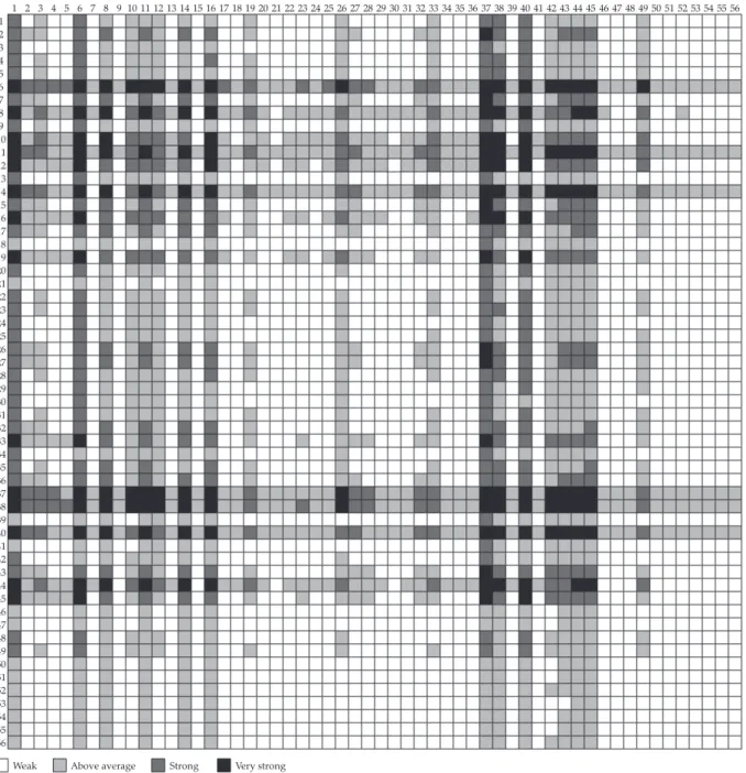
Figure 3 depicts the field of influence calculated in its traditional fashion, (i.e.), without the incorporation of the vector of GHG emissions intensity. This analysis defines the importance of each of the intersectoral relations of purchase and selling. In order to facilitate interpretation, the results for each production link were highlighted in color scales8 indicating the above-average fields of influence, that is, the most important linkages for the economy as a whole. Reading is similar to the input-output matrices, in other words, the lines
Figure 3. Brazilian Economy Field of Influence – 2009
1 2 3 4 5 6 7 8 9 10 11 12 13 14 15 16 17 18 19 20 21 22 23 24 25 26 27 28 29 30 31 32 33 34 35 36 37 38 39 40 41 42 43 44 45 46 47 48 49 50 51 52 53 54 55 56 1
2 3 4 5 6 7 8 9 10 11 12 13 14 15 16 17 18 19 20 21 22 23 24 25 26 27 28 29 30 31 32 33 34 35 36 37 38 39 40 41 42 43 44 45 46 47 48 49 50 51 52 53 54 55 56
Weak Above average Strong Very strong
Source: Own elaboration based on Nereus database (GUILHOTO and SESSO FILHO, 2005, 2010).
are formed by input seller sectors, while the columns are input buyer sectors.
It is noticed that sector 2 – Livestock and Fishing presents few important linkages when compared to other activities. The relations with the sector 37 – Parts and accessories for automotive vehicles are classified as very strong.
Figure 4. Field of Influence weighted by GHG emissions – 2009
1 2 3 4 5 6 7 8 9 10 11 12 13 14 15 16 17 18 19 20 21 22 23 24 25 26 27 28 29 30 31 32 33 34 35 36 37 38 39 40 41 42 43 44 45 46 47 48 49 50 51 52 53 54 55 56 1
2 3 4 5 6 7 8 9 10 11 12 13 14 15 16 17 18 19 20 21 22 23 24 25 26 27 28 29 30 31 32 33 34 35 36 37 38 39 40 41 42 43 44 45 46 47 48 49 50 51 52 53 54 55 56
Weak Above average Strong Very strong
Source: Own elaboration based on Nereus database (GUILHOTO and SESSO FILHO, 2005, 2010).
withthe columns 2 and 24, which highlights the greater intensity of emissions during the production of inputs and outputs. It is noteworthy that these two sectors accounted for 53% of Brazil’s GHG emissions in 2009.
On the other hand, 2 – Livestock and Fishing, and 24 – Cement, as suppliers, have very strong connections along the whole economy. A contribution of this approach is the identification of these two
sectors as the most important on the transmission of GHG intensive inputs to the others sectors. Mitigation of GHG emissions on these sectors could spread to the whole economy.
Demand on the horizontal axis. Supply on vertical axis.
contribution to its generation of employment and income. Nevertheless, one must consider this activity as a significant part of the so-called agribusiness.9 For instance, Montoya et al. (2016) estimated the contribution of agribusiness to the Brazilian GDP at 21% and the contribution to employment generation at 32% in 2009. Taking into account emissions from energy consumption only, the sector was responsible for 40% of the generated CO2 (MONTOYA et al., 2016).
Nevertheless, when Brazil’s emissions are taken into perspective, although the CO2 resulting from the consumption of fossil fuels presents a growth tendency (EPE, 2013; MONTOYA et al., 2016), methane from enteric fermentation and carbon dioxide from slash-and-burn are the greatest part of GHG emissions and are concentrated in Livestock and Fishing. For Bustamante et al. (2012), more than 50% of GHGs are directly or indirectly related to agriculture. Thus, it is relevant to note that although investments in other sectors of the economy generate greater impacts in the productive structure, they have lower GHG emissions levels. The same applies to exports. Indeed, the increase in exports of higher added-value food products over the exports in agriculture can decrease the intensity of emissions from foreign trade (PERUSSO, 2012). Nevertheless, technological changes on Livestock and Fishing, such as the crop and livestock integration, could have major results on mitigation of GHG (MACEDO, 2009) and reduce the GHG intensity on the others economic sectors.
5. Conclusion
The present article has examined the contribution of Livestock and Fishing to the release of GHG in Brazil, taking into account the influence of these emissions
9. The delimitation of agribusiness was accomplished “con-sidering the profound technological, productive, finan-cial and business relationships that agriculture has with industry and other economic activities, the measurement of the agribusiness must be implemented from a systemic view, in which input and output flows and transfers from one sector to another are integrated” (Montoya et al., 2016, p. 387, translation by authors). The aggregation of activ-ities in agribusiness considers the participation of agricul-tural inputs, agriculagricul-tural products, agroindustry products and services related to agriculture; see Finamore and Montoya (2003).
on emissions from other sectors, and vis-à-vis their contribution to the generation of employment and income. To do so, we have used the methodology of the field of influence and impact multipliers applied to the input-output analysis weighted by the coefficients of GHG emissions.
The result indicates that this sector has decisive contributions to the emissions, while its impact on the economic activity is less pronounced. The immediate implication is that investments in other sectors of the economy would result in better economic and environmental performance.
Nevertheless, it is important not to lose sight of the overall importance of agribusiness to the Brazilian economy and of the role that this country shall play in world’s food supply, given its comparative advantages and the growing demand from emerging countries. In this sense, the largest share of higher value-added food in the exportation agenda as substitute for agricultural products may not only favor the generation of employment and income, but also decrease the intensity of emissions from foreign trade.
With the objective of bringing new results to the literature, we intend to perform similar exercises to the ones applied here in future works, but this time considering the economic relations in agribusiness given its relevance to the Brazilian economy.
6. References
AGUIAR, A. P., CÂMARA, G. and ESCADA, M. I. S. Spatial statistical analysis of land-use determinants in the Brazilian Amazonia: exploring intra-regional heterogeneity.Ecological Modelling, v. 209, n. 2-4, p. 169-188, 2007.
BRAZIL. Ministério do Meio Ambiente (MMA).
Informação adicional sobre a INDC. Apenas para fins de esclarecimento. Brasília, 2015, available at http:// mma.gov.br/index.php/comunicacao/agencia-informma?view=blog&id=1163, in 29/09/2015.
BRIZGA, J., FENG, K. and HUBACEK, K. Drivers of greenhouse gas emissions in the Baltic States: a structural decomposition analysis. Ecological Economics, v.98, p. 22-28, 2014.
BUTNAR, I. and LLOP, M. Structural decomposition analysis and input–output subsystems: changes in CO2 emissions of Spanish service sectors (2000-2005).
Ecological Economics, v. 70, p. 2012-2019, 2011.
CARVALHO, T. S., SANTIAGO, F. S. and PEROBELLI, F. S. International trade and emissions: the case of the Minas Gerais state – 2005. Energy Economics, v. 40, p. 383-395, 2013
CASTRO, E. Dinâmica socioeconômica e desmatamento na Amazônia. Novos Cadernos NAEA, v. 8, n. 2, p. 5-39, 2005.
COSTA, C. C., GUILHOTO, J. J. M. and IMORI, D. Importância dos setores agroindustriais na geração de renda e emprego para a economia brasileira. Revista de Economia e Sociologia Rural, v. 51, n. 4, p. 797-814, 2013.
COSTA, F. A. Formação agropecuária da Amazônia: Os desafios do desenvolvimento sustentável. Belém: Núcleo de Altos Estudos Amazônicos v. 1, 2000.
CRISTÓBAL, J. R. S. An environmental/input-output linear programming model to reach the targets for greenhouse gas emissions set by the Kyoto protocol.
Economic Systems Research, v. 22, n. 3, p. 223-236, 2010.
______. A goal programming model for environmental policy analysis: application to Spain. Energy Policy, v. 43, p. 303-307, 2012.
DINIZ, M. B. et al. Causas do desmatamento da Amazônia: uma aplicação do teste de causalidade de Granger acerca das principais fontes de desmatamento nos municípios da Amazônia Legal brasileira. Nova Economia, v. 19, n. 1, p. 121-151, 2009.
EPE – Empresa de pesquisa energética. Plano Decenal de Expansão de Energia 2022. Brasília, Ministério das Minas e Energia, 2013.
FAO – Food and Agriculture Organization of the United Nations. Global forest resources assessment 2010, 2010.
FEARNSIDE, P. M. Deforestation in Brazilian Amazonia: history, rates and consequences. Conservation Biology, v. 19, n. 3, p. 680-688, 2005.
FINAMORE, E. B. and MONTOYA, M. A. PIB, tributos, emprego, salários e saldo comercial no agronegócio gaúcho. Ensaios FEE, v. 24, n. 1, p. 93-126, 2003.
GOLDEMBERG, J. and GUARDABASSI, P. M. Climate change and historical responsibilities. Ambiente & Sociedade, v. 15, n. 1, p. 201-206, 2012.
GUILHOTO, J. J. M. and SESSO FILHO, U. Estimação da matriz insumo-produto a partir de dados preliminares das contas nacionais. Economia Aplicada, v. 9, n. 2, p. 277-299, 2005.
GUILHOTO, J. J. M. and SESSO FILHO, U. A. Estimação da matriz insumo-produto utilizando dados preliminares das Contas Nacionais: aplicação e análise de indicadores econômicos para o Brasil em 2005.
Revista Economia & Tecnologia, v. 6, n. 4, p. 53-62, 2010.
HETTIGE, H. et al. The Industrial Pollution Projection System (IPPS). Policy Research Working Paper, n. 1431, Part 1 and 2, 1994.
HOUGHTON, R. A. Aboveground forest biomass and the global carbon balance. Global Change Biology, v. 11, n. 6, p. 945-958, 2005.
HRISTU-VARSAKELIS, D. et al. Optimizing production with energy and GHG emission constraints in Greece: An input-output analysis. Energy Policy, v. 38, n. 3, p. 1566-1577, 2010.
HRISTU-VARSAKELIS, D. et al. Optimizing production in the Greek economy: exploring the interaction between greenhouse gas emissions and solid waste via input–output analysis. Economic Systems Research, v. 24, n. 1, p. 55-75, 2012
IPCC – International Panel on Climate Change.
Climate change 2001: the scientific basis. Contribution of working group I to the third assessment report of the intergovernmental panel on climate change. Cambridge, UK: Cambridge University Press, 2001.
JANZEN, H. H. Carbon cycling in earth systems – a soil science perspective. Agriculture, Ecosystems and Environment, v. 104, n. 3, p. 399-417, 2004.
LENZEN, M. et al. Drivers of change in Brazil’s carbon dioxide emissions. Climatic Change, v. 121, n. 4, p. 815-824, 2013.
LEONTIEF, W. The structure of the American economy, 1919-1939: an empirical application of equilibrium analysis. Oxford University Press: New York, 1941.
LOYOLA, G. Perspectivas para o mercado de proteína animal. Tendências consultoria. Apresentação para o Congresso Internacional de Carnes, Goiânia (GO). Available online at <http://www.congressodacarne2013.com.br/ palestras/Gustavo%20Loyola.pdf>, 2013.
MACEDO, M. C. M. Integração lavoura e pecuária: o estado da arte e inovações tecnológicas. Revista Brasileira de Zootecnia, v. 38, p. 133-146, 2009.
MARGULIS, S. Causas do desmatamento da Amazônia brasileira. Brasília: Banco Mundial, 2003.
MCTI – Ministério da Ciência, Tecnologia e Inovação.
______. Estimativas anuais das emissões de gases de efeito estufa no Brasil. MCTI, 2013.
MILLER, R. E. and BLAIR, P. D. Input-output analysis: foundations and extensions. 2. ed. New York: Cambridge University Press, 2009.
MMA – Ministério do Meio Ambiente. Plano de prevenção e controle do desmatamento na Amazônia Legal. Available online at <http://www.mma.gov.br/ florestas/controle-e-preven%C3%A7%C3%A3o-do- desmatamento/plano-de-a%C3%A7%C3%A3o-para-amaz%C3%B4nia-ppcdam>. 2013.
MOLL, S. et al. Environmental input-output analysis based on NAMEA data. A comparative European study on environmental pressures arising from consumption and production patterns European topic center on resource and waste management: European Environment Agency, 2006.
MONTOYA, M. A. et al. Consumo de energia, emissões de CO2 e a geração de emprego e renda no agronegócio brasileiro: uma análise insumo-produto. Economia Aplicada, v. 20, n. 4, p. 383-412, 2016.
MOSIER, A. R. et al. Mitigating agricultural emissions of methane. Climatic Change, v. 40, n. 1, p. 39-80, 1998.
NEPSTAD, D. et al. Road paving, fire regime feedbacks, and the future of Amazon forests.Forest Ecology and Management, v. 154, n. 3, p. 395-407, 2001.
PERUSSO, A. Reduction in carbon emissions in the Brazilian agricultural value chain through a decrease in transported volume. International Journalof Green Economics, v. 6, n. 4, p. 390-400, 2012.
PRODES/INPE – Projeto de monitoramento da Floresta Amazônica por satélites. Instituto Nacional de Pesquisas Espaciais. Available online at <www.inpe.br>, 2014.
RHEE, H-C. and CHUNG, H-S. Change in CO2emission and its transmissions between Korea and Japan using international input–output analysis.
Ecological Economics, v. 58, p. 788-800, 2006.
RIVERO, S. et al. Pecuária e desmatamento: uma análise das principais causas diretas do desmatamento na Amazônia. Nova Economia, v. 19, n. 1, p. 41-66, 2009.
SILVA, M. P. N. and PEROBELLI, F. S. Efeitos tecnológicos e estruturais nas emissões brasileiras de CO2 para o período 2000 a 2005: uma abordagem de análise de decomposição estrutural (SDA). Estudos Econômicos, v. 42, n. 2, p. 307-335, 2012.
SMITH, K. A. and CONEN, F. Impacts of land management on fluxes of trace greenhouse gases.Soil Use and Management, v.20, n. 2, p. 255-263, 2004.
SONIS, M. and HEWINGS, G. J. D. Coefficient change in input–output models: Theory and applications.
Economic Systems Research, v. 4, n. 2, p. 143-158, 1992.
SU, B., ANG, B. W. and LOW, M. Input–output analysis of CO2 emissions embodied in trade and the driving forces: processing and normal exports. Ecological Economics, v. 88, p. 119-125, 2013.
YAMAKAWA, A. and PETERS, G. P. Structural decomposition analysis of greenhouse gas emissions in Norway 1990–2002. Economic Systems Research, v. 23, n. 3, p. 303-318, 2011.
YOUNG, C. E. F. Potencial de crescimento da economia verde no brasil. Política Ambiental. Economia verde: desafios e oportunidades, n. 8, p. 88-97, 2011.
WRI – World Resources Institute. Data visualizations. Available online at <http://www.wri.org/resources/ data_visualizations>. 2014.