A Convergence Indicator for Multi-Objective Optimisation Algorithms

(1)

doi: 10.5540/tema.2018.019.03.0437

A Convergence Indicator for

Multi-Objective Optimisation Algorithms

T. SANTOS and S. XAVIER

Received on January 26, 2018 / Accepted on April 16, 2018

ABSTRACT. The algorithms of multi-objective optimisation had a relative growth in the last years. Thereby, it requires some way of comparing the results of these. In this sense, performance measures play a key role. In general, it’s considered some properties of these algorithms such as capacity, convergence, diversity or convergence-diversity. There are some known measures such as generational distance (GD), inverted generational distance (IGD), hypervolume (HV), Spread(∆), Averaged Hausdorff distance (∆p),

R2-indicator, among others. In this paper, we focuses on proposing a new indicator to measure conver-gence based on the traditional formula for Shannon entropy. The main features about this measure are: 1) It does not require to know the true Pareto set and 2) Medium computational cost when compared with Hypervolume.

Keywords: Shannon Entropy, Performance Measure, Multi-Objective Optimisation Algorithms.

1 INTRODUCTION

Nowadays, the evolutionary algorithms (EAs) are used to obtain approximate solutions of multi-objective optimisation problems (MOP) and these EAs are called multi-multi-objective evolutionary algorithms (MOEAs). Some of these algorithms are very well-known among the community such that NSGA-II (See [1]), SPEA-II (See [2]), MO-PSO (See [3]) and MO-CMA-ES (See [4]). Although the most of MOEAs to use the previous criteria, whenm>3 the MOP is called

Many Objectives Optimization Problemsand in this case algorithms Pareto-Based is not good enough. Some papers try to explain the reason why such thing happens (See [5, 6]). To avoid the phenomenon caused by Pareto relation, some researchers indicates others way of comparative the elements (See [7]) or change into Non-Pareto-based MOEAs, such as indicator-based and aggregation-based approaches (See [8, 9]).

With the MOEAs in mind, it’s natural to know how theirs outputs are relevant. According the [10], it was listed 23 indicators which intend to provide us some information about this such as

*Corresponding author: Thiago Santos – E-mail:santostf@gmail.com

(2)

algorithms. Those indicators have basically three goals, that is: 1) Closeness to the theoretical Pareto set, 2) Diversity of the solutions or 3) number of Pareto-optimal solutions. Build an in-dicator which give us information about all those three goals above it is something tough to do it. However, there are great ways to measure the quality in this path. The most used one, it is the Inverted Generational Distance (IGD) and Generational Distance (GD)(see [11]) because of simplicity and low cost to calculate. Recently, another one based on this measure was propose so called Hausdorff Measure (see [12]) which combines the IGD and GD and takes its maximum. These indicator is efficient to obtain informations about closeness of the output of some algo-rithm with the True Pareto set. The difficult here is because in the order to calculate the IGD/GD it’s necessary to know the True Pareto Set of the problem and some ( or the most of time) such as information it’s not available. Another one, very well-know, is the Hypervolume or S-metric (see [13]). The main problem with this indicator is related with its huge computational cost and to avoid this some authors suggest to use Monte Carlo Simulation to approximate the value and decrease the cost (see [14]).

Here, we will be providing an indicator which allow us talk about nearness of the True Pareto Set. The idea comes from the [15] what introduce a great function that satisfies the KKT conditions. With this function, we do not need to know anything about the exact solutions of the problem or needs to choose a right reference point.

The paper is organised as follow: on section 2 we establish the general multi-objective problem and on 3 we talk about three well-known indicators. Finally, on section 4 we presents our idea and on 5 we do some numeral simulations.

2 MULTI-OBJECTIVE PROBLEM (MOP)

It’s common to define multi-objective optimisation problems (MOP) as follows:

minf(x), f(x) = (f1(x),f2(x),· · ·,fm(x))

s.t: x∈Ω⊂Rn (2.1)

in whichx∈Rn

is thedecision variable vector, f(x)∈Rm

is theobjective vector, andΩ⊆Rn is thefeasible setthat we consider as compact and connected region. In this work, we assumed here that the functions fi(·)are continuously differentiable (orC2(Ω)).

The aim of multi-objective optimisation is to obtain an estimate of the set of points belonging to

Ωwhich minimize, in the certain sense that we will call by Pareto-optimality.

Definition 1.Let u,v∈Rm_{. We say that u dominates v, denoted by u}_{v, iff} _∀i₌₁_{, . . . ,}_m

(3)

Definition 2.A feasible solution x∗∈Ωis a Pareto-optimal solution of problem (2.1) if there is no x∈Ωsuch that f(x)f(x∗). The set of all Pareto-optimal solutions of problem(2.1)is called by Pareto Set (PS) and the its image is the Pareto Front (PF). Thus,

PS = {x∈Ω|∄y∈Ω,f(y)f(x)} PF = {f(x)|x∈PS}

A classical work (See [16]) established a relationship between the points of PS and gradient in-formations from the problem (2.1). That connection it is known by Karush-Kuhn-Tucker (KKT) conditions for Pareto optimality that we define as follow:

Theorem 1 (KKT Condition [16]). Let x∗∈ PS of the problem(2.1). Then, there exists

nonnegative scalarsλ_i_≥₀_{, with} m

∑

i=1

λ_i₌₁_{, such that}

m

∑

i=1

λ_i∇fi(x∗) =0 (2.3)

This theorem will be fundamental to this paper because we will use this fact to formulate our proposal.

3 SOME CONVERGENCE INDICATORS

In this section, we will go to relate some metrics or indicators known by scientific community and well-done established. The idea here is to compare those indicators further below with our proposal measure.

3.1 GD/IGD

The Inverted Generational Distance (IGD) indicator has been using since 1998 when it was cre-ated. The IGD measure is calculated on objective space, which can be viewed as an approximate distance from the Pareto front to the solution set in the objective space. In the order to define this metric, we assume that the setΛ={y1,y2,· · ·,yr}is an approximation of the Pareto front for the problem (2.1). Let be theVMOEAa solutions set obtained by some MOEA in the objective space asVMOEA={v1,v2,· · ·,vk}wherevi is a point in the objective space. Then, the IGD metric is calculated for the setVMOEAusing the reference pointsΛas follows:

IGD(VMOEA,Λ) = 1

r

∑

i=1

d(yi,VMOEA)2 !1/2

, (3.1)

whered(y,X)denotes the minimum Euclidean distance betweenyand the points inX. Besides, we also can to define deGDmetric by

(4)

This indicators are measure representing how ”far” the approximation front is from the true Pareto front. Lower values of GD/IGD represents a better performance. The only different between GD and IGD is that in the last one you don’t miss any part true Pareto set on comparison.

In [17] indicates two main advantages about it: 1) its computational efficiency even many-objective problems and 2) its generality which usually shows the overall quality of an ob-tained solution set. The authors in [17] studied some difficulties in specifying reference points to calculate the IGD metric.

3.2 Averaged Hausdorff Distance(∆_p)

This metric combine generalized versions ofGDandIGDthat we denote byGDp/IGDpand defined by, with the same previous notation,

IGD(VMOEA,Λ)p = 1

r

∑

i=1

d(yi,VMOEA)p !1/p

(3.3)

GD(VMOEA,Λ)p = IGD(Λ,VMOEA)p (3.4)

The indicator, so called by∆_p, was proposed in [12] defined by

∆p(X,Y) =max{IGD(X,Y)p,GD(X,Y)p}, (3.5)

In [12] the author proved that function is a semi-metric,∆_pdoes not fill the triangle inequality, for 1≤p<∞. Many others properties was proved in [12].

3.3 Hypervolume (HV)

This indicator has been using by the community since 2003. Basically, the hypervolume of a set of solutions measures the size of the portion of objective space that is dominated by those solutions as a group. In general, hypervolume is favored because it captures in a single scalar both the closeness of the solutions to the optimal set and, to some extent, the spread of the solutions across objective space. There are many works on this indicator such as in [13] which the author studied how expensive to calculate this indicator was. Few years later, it was proposed a faster alternative by using Monte Carlo simulation ( See [14]) that it was addressed for many objectives problem by Monte Carlo simulation. In the order to get a right definition, you can look at [14, 13].

4 PROPOSAL MEASUREH

In the order to define our proposal measure, consider the quadratic optimization problem (4.1) associated with (2.1):

min

α_∈Rn    m

∑

i=1

α_i∇fi(x) 2

; α_i_≥₀_, m

∑

i=1 α_i₌₁

 

(5)

The existence and uniqueness of a global solution of the problem (4.1) is stabilised in [15]. The functionq:Rn→Rn

given by

q(x) =

m

∑

i=1 b

α_i∇f_i(x) (4.2)

whereαb_{is a solution of the (4.1), becomes well defined. There is a interested property about this} function that was proved in [15]:

• each x∗ withkq(x∗)k2=0, where| · | represents euclidean norm, fulfills the first-order necessary conditions for Pareto optimality given by Theorem 1.

Thereby, these points are certainly Pareto candidates what motivates the next definition about nearness.

Definition 3.A point x∈Ωis calledε_{−closed to Pareto set if}_kq₍_x∗₎_k2_<ε_.

Let the setX={x1,x2,· · ·,xk}the output from some evolutionary algorithms. With the feature about that function, we can to define a new measure by:

H₍X):= 1

2k

k

∑

i=1

−qilog2(qi) (4.3)

whereqi=min{1/exp(1),kq(xi)k2}and put 0·log2(0) =0.

The expression (4.3) is the traditional formula used for Shannon Entropy( See [18]). Unlike the original way that is used this as a entropy, in the our metric each qi is not to related with a probability space.

Theorem 2.About the function in(4.3), we have that

0≤H₍X)≤1

2

log₂(e1)

e1 (4.4)

Proof. First, since 0≤qi≤0.5 thenH(X)≥0. On the other hand, it is known that the function

f(x) =−xlog2(x)has a maximum atx=1/exp(1), hence

H₍X) = 1

2k

k

∑

i=1

−qilog2(qi)

≤ 1

2k

k

∑

i=1

−exp(−1)log₂(exp(−1))

≤ 1

2k(k)(exp(−1)log2(exp(1))

= 1

2

log2(exp(1))

(6)

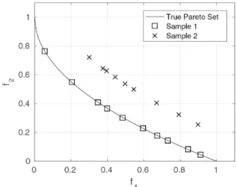
Figure 1: Empirical Idea to illustrateH_.

A reasonable the interpretation of aboutH₍_·₎_{might be:}₍a)whetherH₍X)closed to or equal 0 then the setXhas a good convergence to the Pareto Set;(b)whetherH₍_X₎_{closed to or equal}

0.26537 then the setX does not convergence to Pareto Set.

The main features associated with this metric are: 1) The true Pareto set doesn’t require to be predefined and 2) It can be to used with many-objectives problems. The first point is important because it is almost impossible to know the true PF in general. On the other hand, the second attribute is useful since it doesn’t exists many indicator to be used in this problems.

In the figure (1), we have an empirical with two samples that supposed approximates the true Pareto set (PF). Intuitively, we can say that the sample 1 is more closed to PF than sample 2. If it were calculated IGD/GD metric, the sample 1 we will get values more near the zero than sample 2. Also we have the same conclusion with our proposal.

4.1 Computational Complexity

To calculateH_{, the major computational cost is related with calculation of function}qbecause we have that previously to find the solution of (4.1). This requires O₍_m_·_n₎_{computations to}

compute it. Consequently, the overall complexity needed isO₍_m_·_n_·_k₎_.

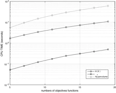
The aim behind of figures (2) and (3) it’s to show a comparative with others metrics by measuring CPU time. We conducted the experiment on Intel Core I7 with 16gb RAM and we used the traditional benchmark function DTLZ2 (see [19]).

(7)

did for the calculation the HV in this case. On the other hand, for the simulation on figure (3), we configured popSize as 50∗Mand size of exact population as 100∗MwhereMis the number of objectives function on each run.

Figure 2: CPU TIME( in logarithmic scale) versus size of population.

(8)

Figure 4: Entropy measure is computed for non-dominated solutions of MOPSO-cd populations for Problem ZDT2.

Both tests showed us a most cost for calculating of the our indicator in relation the∆_pbut rela-tively less when we compare with the calculation of HV. A fact that already was expected because of the equation (4.1) as we pointed out earlier. Nevertheless, from the figure (3), it is possible to conclude by CPU time that for many objectives problems our proposal is acceptable in relation with the HV.

The figure (4) shows the behavior ofH _{with the non-dominated solutions of MOPSO-cd}

algo-rithm (see [20]) for the benchmark function ZDT2. Through this experiment, which was fixed 105 evaluation function, it is possible to see that the values of this measure decrease mono-tonically. Actually, this property comes from the continuity and monotonicity of the function

f(x) =−xlog2(x)into the interval[0,1/e1].

5 SIMULATION RESULTS

The aim here is to compare our proposal with other indicators presented previously, i.e,∆₂e HV. Besides, we have been chosen benchmark DTLZ ( DTLZ1, DTLZ2, DTLZ5 and DTLZ7) due the facility of its scalarization. We have decided for the three well-known algorithms which the setup follow below:

1. MOPSO-CD (See [20] )

2. NSGA-II (See [1])

(9)

In both algorithms, we fixed the output population in 100 individuals with three objectives func-tions and we ran 30 times with 25000 function evaluafunc-tions running in each one. We have leaded this experiment on PlatEMO framework (See [22]).

Table 1: DTLZ1 function results

∆₂ HV H

NSGA-II 0.030712 ( 0.024266 ) 1.296030 ( 0.027097 ) 0.246989 ( 0.006442 ) NSGA-III 0.021337 ( 0.001355 ) 1.303803 ( 0.000829 ) 0.226985 ( 0.002771 ) MOPSO-CD 8.760441 ( 2.893284 ) 0.007216 ( 0.039522 ) 0.262165 ( 0.005288 )

∆₂ HV H

∆2 HV H

Throughout the tables (1), (2) and (3) we can conclude the same thing with all indicator, included our proposal as it was expected by the previous section.

6 CONCLUSIONS

In this paper, we have introduced a new indicatorH _{which goal is evaluate the outcome from}

an evolutionary algorithm on the Multi-objective optimisation problems. We have tested the new approach with some classic benchmark and make a comparative with some others indicators that is already known. By experimental results, we can to conclude the same what is indicated by the other indicators of performance. Unlike such these indicators, our proposal needs to known nothing about the true Pareto of set of the MOP. This features, we consider a great to thing because most MOPs is doesn’t have this information.

(10)

ACKNOWLEDGMENT

The authors would like to be thankful for the FAPEMIG by financial support to this project.

RESUMO. Os algoritmos de otimização multi-objectivo tiveram um relativo crescimento nos últimos anos. Diante disso, é necessária alguma maneira de comparar os resultados por eles gerados. Neste sentido, medidas de desempenho são importantes. Em geral, são con-sideradas algumas propriedades desses algoritmos tais como capacidade, convergência, di-versidade ou convergência-didi-versidade. Algumas dessas medidas são conhecidas da comu-nidade acadêmica como generational distance (GD), inverted generational distance (IGD), hypervolume (HV), Spread(∆), Averaged Hausdorff distance (∆p), R2-indicator dentre

out-ros. Aqui, nós focamos em propor um novo indicador para medir a convergência baseada na formula tradicional da entropia de Shannon. As principais caracter´ısticas da nossa proposta são: 1) Não depende de saber o conjunto Pareto Exato e 2)Médio custo computacional quando comparado com o Hypervolume.

Palavras-chave:Entropia de Shannon, Medidas de desempenho, Algoritmos de otimizac¸˜ao multi-objectivo.

REFERENCES

[1] K. Deb, A. Pratap, S. Agarwal, and T. Meyarivan, “A fast and elitist multiobjective genetic algorithm: NSGA II,”IEEE Trans. Evol. Comp., vol. 6, no. 2, pp. 182–197, 2002.

[2] E. Zitzler, M. Laumanns, and L. Thiele, “Spea2: Improving the strength pareto evolutionary algorithm,” tech. rep., 2001.

[3] C. A. Coello Coello and M. S. Lechuga, “Mopso: A proposal for multiple objective particle swarm optimization,” inProceedings of the Evolutionary Computation on 2002. CEC ’02. Proceedings of the 2002 Congress - Volume 02, CEC ’02, (Washington, DC, USA), pp. 1051–1056, IEEE Computer Society, 2002.

[4] C. Igel, N. Hansen, and S. Roth, “Covariance matrix adaptation for multi-objective optimization,”

Evol. Comput., vol. 15, pp. 1–28, Mar. 2007.

[5] T. Santos and R. H. C. Takahashi, “On the performance degradation of dominance-based evolutionary algorithms in many-objective optimization,”IEEE Transactions on Evolutionary Computation, Nov 2016.

[6] O. Schutze, A. Lara, and C. A. C. Coello, “On the influence of the number of objectives on the hardness of a multiobjective optimization problem,”IEEE Transactions on Evolutionary Computation, vol. 15, pp. 444–455, Aug 2011.

[7] B. Li, J. Li, K. Tang, and X. Yao, “Many-objective evolutionary algorithms: A survey,”ACM Comput. Surv., vol. 48, pp. 13:1–13:35, Sept. 2015.

(11)

Conference on Genetic and Evolutionary Computation, GECCO ’10, (New York, NY, USA), pp. 527– 534, ACM, 2010.

[9] T. Wagner, N. Beume, and B. Naujoks, “Pareto-, aggregation-, and indicator-based methods in many-objective optimization,” inProceedings of the 4th International Conference on Evolutionary Multi-criterion Optimization, EMO 07, (Berlin, Heidelberg), pp. 742–756, Springer-Verlag, 2007.

[10] A. Zhou, B.-Y. Qu, H. Li, S.-Z. Zhao, P. N. Suganthan, and Q. Zhang, “Multiobjective evolutionary algorithms: A survey of the state of the art.,”Swarm and Evolutionary Computation, vol. 1, no. 1, pp. 32–49, 2011.

[11] P. Czyzak and A. Jaszkiewicz, “Pareto simulated annealing - a metaheuristic technique for multiple-objective combinatorial optimization,” Journal of Multi-Criteria Decision Analysis, vol. 7, no. 1, pp. 34–47, 1998.

[12] O. Schutze, X. Esquivel, A. Lara, and C. A. C. Coello, “Using the averaged hausdorff distance as a performance measure in evolutionary multiobjective optimization,”IEEE Trans. Evol. Comp, vol. 16, pp. 504–522, Aug. 2012.

[13] L. While, P. Hingston, L. Barone, and S. Huband, “A faster algorithm for calculating hypervolume,”

IEEE Transactions on Evolutionary Computation, vol. 10, pp. 29–38, Feb 2006.

[14] J. Bader and E. Zitzler, “Hype: An algorithm for fast hypervolume-based many-objective optimization,”Evol. Comput., vol. 19, pp. 45–76, Mar. 2011.

[15] S. Schaffler, R. Schultz, and K. Weinzierl, “Stochastic method for the solution of unconstrained vector optimization problems,”J. Optim. Theory Appl., vol. 114, pp. 209–222, July 2002.

[16] H. W. Kuhn and A. W. Tucker, “Nonlinear programming,” inProceedings of the Second Berkeley Symposium on Mathematical Statistics and Probability, (Berkeley, Calif.), pp. 481–492, University of California Press, 1951.

[17] H. Ishibuchi, H. Masuda, Y. Tanigaki, and Y. Nojima, “Difficulties in specifying reference points to calculate the inverted generational distance for many-objective optimization problems,” in Com-putational Intelligence in Multi-Criteria Decision-Making (MCDM), 2014 IEEE Symposium on, pp. 170–177, Dec 2014.

[18] R. M. Gray,Entropy and Information Theory. New York, NY, USA: Springer-Verlag New York, Inc., 1990.

[19] K. Deb, L. Thiele, M. Laumanns, and E. Zitzler, “Scalable Multi-Objective Optimization Test Problems,” inCongress on Evolutionary Computation (CEC 2002), pp. 825–830, IEEE Press, 2002.

[20] C. R. Raquel and P. C. Naval, Jr., “An effective use of crowding distance in multiobjective parti-cle swarm optimization,” inProceedings of the 7th Annual Conference on Genetic and Evolutionary Computation, GECCO ’05, (New York, NY, USA), pp. 257–264, ACM, 2005.

(12)