MASTER IN ELECTRICAL AND COMPUTERSENGINEERING
Adaptation of an Harp for MIDI Implementation and
Sound Amplification
MASTER THESIS DISSERTATION
Author:
João Miguel A. Beleza
Supervisor:
Prof. Aníbal Ferreira
Abstract
The objective for this thesis project will be to adapt an Harp for MIDI imple-mentation together with sound amplification. To accomplish that objective, this project will focus on studying all available products that can provide these functionalities with the intention of developing its own product while remaining competitive in the mar-ket. To define priorities the MIDI implementation will be the main focus of the project while the sound amplification will be the secondary objective.
This thesis dissertation will aim to provide a walk through process justifying all the decision making regarding both implementations. The first step will be to study and develop tools that allow data to be collected from any device chosen. Secondly, this project will focus on the study of piezoelectric transducers in order to make the bridge between the string vibration of the harp and the corresponding electrical signal. Following this analysis, the MIDI implementation will be developed using the already established transducers mechanism together with the sound amplification system. Fi-nally, a very brief market analysis justifying and validating the product will take place for the finalized product.
Resumo
O objetivo para este projeto de Tese será adaptar uma harpa para implemen-tação MIDI em conjunto com amplificação sonora. De modo a cumprir este objetivo, este projeto irá primeiramente focar-se no estudo de todos os produtos disponíveis no mercado capazes de realizar tais funcionalidades. Este estudo servirá como base para desenvolver um protótipo funcional competitivo no mercado actual. De modo a definir prioridades a implementação MIDI servirá como foco principal do projeto e a amplificação sonora será o objetivo secundário.
Esta dissertação irá focar-se em providenciar uma descrição passo a passo da maioria das decisões tomadas para desenvolver ambas as implementações. O primeiro passo será estudar e desenvolver ferramentas que permitam recolher e guardar dados dos dispositivos escolhidos. De seguida, este projeto irá focar-se no estudo de transdu-tores piezoelétricos que permitam fazer a ponte entre a vibração das cordas da harpa e do correspondente sinal elétrico. Posterior a esta análise, a implementação MIDI em conjunto com a implementação de áudio será desenvolvida utilizando o mecanismo desenvolvido. Por fim, uma muito breve análise de mercado será fornecida de forma a validar e justificar o produto final.
Acknowledgements
I would like to thank my coordinator Prof. Aníbal João de Sousa Ferreira who not only accepted and made possible the initial proposal as well as helping and guid-ing me throughout the whole project development. I would like to thank my family especially my mother, Maria do Rosário Beleza, and my father, Álvaro Manuel Beleza, for supporting me in this project as well as my grandfather, José Antonino Beleza, who helped me develop many of the more practical aspects of this endeavour.
I would also like to thank my friends who made all the effort possible through good and bad moments of this project, those who are in my heart, those who are not here, those who kept me from failing and those who lend their ear. A special thanks to the girl with sapphires, the LM couple, the best work partner I have ever had, the future harpmaker and the best friend this man has had, you all made all of this possible.
Contents
1 Introduction 1
1.1 Brief Context . . . 1
1.1.1 Sound to Midi Conversion . . . 1
1.1.2 Introduction to the Harp . . . 2
1.2 Motivation for MIDI adaptation of an Harp . . . 4
1.3 Main Objetives . . . 5 2 Fundamentals Overview 7 2.1 Approach Comparison . . . 7 2.1.1 MIDI Conversion . . . 7 2.1.2 Sound Amplification . . . 9 2.2 Fundamentals . . . 10 2.2.1 Sound Transducers . . . 10 2.2.2 MIDI Conversion . . . 16 2.2.3 Sound Amplification . . . 18 3 Inital Approach 21 3.1 Discrete Objectives . . . 21 3.2 Initial Methods . . . 22 4 Work Methodology 25 4.1 Project Phases . . . 25 4.1.1 Preparation Phase . . . 25 4.1.2 Developing Phase . . . 26 4.2 Project Tools . . . 27
5 Research Methods and Developed Tools 29 5.1 Research Tools . . . 29 5.1.1 Oscilloscope . . . 29 5.1.2 Multisim . . . 29 5.1.3 Developed Software . . . 30 5.2 Teensy Microcontroller . . . 31 5.2.1 Characteristics . . . 31
5.2.2 Teensy and Python oscilloscope - Validation of a Single ADC . . 31
5.2.3 Teensy and Python oscilloscope - Validation of a Both ADCs . . . 35
6 Piezoelectric Transducer 40
6.1 Concept and Initial Design . . . 40
6.2 Piezoelectric Disk Testing . . . 43
6.3 Contact Hollow Cylinder Testing . . . 45
6.4 Full schematic Testing . . . 46
7 MIDI Adaptation 50 7.1 Objectives for MIDI Implementation . . . 50
7.2 Concept Design . . . 51
7.2.1 Signal Rectification and Conditioning . . . 51
7.2.2 RC Pair . . . 53
7.2.3 Capturing MIDI OFF . . . 59
7.2.4 Active Alternative . . . 61
7.2.5 Timings and MIDI Implementation . . . 65
7.2.6 Comparison of both Models and Final Considerations . . . 67
8 Audio Amplification 70 8.1 Objectives for Audio Amplification . . . 70
8.2 Concept Proposal . . . 71
8.2.1 Initial Signal Conditioning . . . 72
8.2.2 Filtering and Effects . . . 74
8.2.3 Final Gain . . . 75
9 Conclusion and Result Analysis 78 9.1 Brief Market Evaluation . . . 78
9.2 Result Analysis . . . 79
9.3 Optimizations . . . 81
10 References 82
A Teensy and Python Response Times 86
List of Figures
1 Celtic Harp . . . 3
2 Pedal Harp . . . 3
3 Schematic of the System of a Pedal Harp . . . 3
4 Overview of the Problem . . . 7
5 MIDI implementation on a regular harp . . . 8
6 MIDI implementation on a non regular harp . . . 8
7 Piezo voltage response to an applied voltage or mechanical force . . . . 10
8 Capacitive behaviour of a Piezo Element . . . 12
9 Equivalent Piezo circuit model . . . 12
10 Frequency response of a piezo element . . . 13
11 Impedance per frequency response of a piezo element . . . 13
12 Resonance frequency by piezo shape . . . 15
13 Typical piezo response . . . 16
14 Simplified peak acquisition . . . 16
15 Example of a MIDI message . . . 17
16 First Stage Amplification Example . . . 19
17 Example of the timing window for Medium Sampling and Conversion Speed at 12 bits . . . 34
18 Complex Waveform . . . 36
19 Decomposed Waveform . . . 36
20 Fast Fourier Transform . . . 36
21 Spectral Leakage without windowing . . . 37
22 Spectral Leakage with windowing . . . 37
23 Hamming Windowing . . . 38
24 Blackman-Harris Windowing . . . 38
25 Frequency Response of Piezo PIC 255-0753 . . . 41
26 Results of the Cuboid Piezo element using metal contact . . . 42
27 Side View of the Piezo Structure . . . 43
28 Top View of the Piezo Structure . . . 43
29 Piezo Result of medium pluck with FFT . . . 44
30 Amplified Piezo Result of medium pluck with FFT . . . 44
31 Piezo Result of stronger pluck with FFT . . . 44
32 Piezo Result of medium pluck with FFT . . . 45
33 Amplified Piezo Result of medium pluck with FFT . . . 45
36 Piezo Result of medium pluck with FFT . . . 47
37 Piezo Result of strong pluck with FFT . . . 47
38 Amplified Piezo Result of medium pluck . . . 47
39 Idealization of a piezo Circuit Adaptation for a MIDI Implementation . . 51
40 Natural piezo response to a a small pluck . . . 51
41 Natural piezo response to a a strong pluck . . . 51
42 Rectification using One Diode . . . 52
43 Rectification using Two Diodes . . . 52
44 Idealization of Piezo circuit with piezo schematic . . . 53
45 Medium pluck read by the oscilloscope . . . 54
46 Medium pluck read by the microcontroller . . . 54
47 Results of a high output resistance . . . 54
48 Results of a low output resistance for a strong pluck . . . 54
49 Example of low sampling speeds and lost peak information . . . 55
50 Results of a good quality peak capture, high sampling rate . . . 56
51 Results of a low quality peak capture, low sampling rate . . . 56
52 Results of a 50kHzsample rate . . . 58
53 Results of a 3kHzsample rate . . . 58
54 Results of a string vibration block . . . 59
55 Resuslts of a string vibration natural tendency with DC . . . 60
56 Amplified results of a string vibration block with DC . . . 60
57 Final implementation of passive circuit . . . 60
58 Resuslts of a 4 consecutive plucks using the same force . . . 61
59 Results of 4 consecutive pluck with decreasing force . . . 61
60 Initial Idealization for an Active MIDI implementation . . . 61
61 Amplified Output (green) compared to a non-amplified output (yellow) 63 62 Natural output noise on the ADC . . . 64
63 Result of a slightly blocked string . . . 64
64 Final implementation of the active circuit . . . 64
65 Idealization of a piezo Circuit Adaptation for an Audio Implementation 71 66 Attenuated DC (green) compared to non attenuated DC (yellow) . . . . 72
67 Frequency Response using R1 = 100Ω . . . 73
68 Frequency Response using R1 = 22kΩ . . . 73
69 Frequency Response using R1 = 55kΩ . . . 73
70 Comparison between a clipped and non clipped signal . . . 75
71 Comparison between a clipped and non clipped signal amplified . . . . 75
72 ADC Results for a 3 Volts Peak to Peak Wave at 5kHz . . . 87
73 ADC results for a 50 mVolts Peak to Peak Wave at 5kHz . . . 88
74 ADC results for a 1, 2 and 3 Volts Peak to Peak Wave at 5kHz using 16 bit Resolution, Very High Sampling Speed and Medium Conversion Speed 89 75 Timings schematic for MIDI implementation . . . 94
List of Tables
1 Version Control. . . xviii 2 Timing Response of the MIDI Implementation . . . 66 3 Power Consumption of the MIDI Implementation . . . 67 4 Rough estimation of Final Fabrication Price for a final Implementation
in euros . . . 78 5 Teensy ADC and Serial Interface Response Times . . . 86 6 Average ADC and Serial Interface Response Time for concurrent tests
realized in Figure 74 . . . 89 7 Average ADC Response Time for Single Measurements using no
Aver-aging and 12 bit Resolution . . . 90 8 Average ADC Response Time for Single Measurements using no
Aver-aging and 16 bit Resolution . . . 91 9 Average ADC Response Time for Single Test with an increasing averaging 92
Abbreviatures and Symbols
Piezo Piezoelectric
ADC Analog to Digital Converter DAC Digital to Analog Converter DIY Do IT Yourself
FT Fourier Transform
DFT Discrete Fourier Transform FFT Fast Fourier Transform
MΩ megaOhm kΩ kiloOhm Ω Ohm µs microSecond ms miliSecond V Voltage Vpp Voltage peak-to-peak F Farad pF picoFarad µF microFarad
Version Control
Version Date
Changes / Motivation
1.0 02/02/19 Document Creation1.1 10/02/19 Validation of Preliminary Document 2.0 18/06/19 Final Thesis First Submission
2.1 22/06/19 Final Thesis First Validation 3.0 23/06/19 Final Thesis Validated
1
Introduction
This section will approach the subject of Sound to Midi conversion regarding its context, motivation, application and overall use cases. Consecutively, an introduction will be provided to the harp as an instrument with regards to its purpose and usage. In conclusion a relation between these two topics will be provided justifying the project’s motivation and objectives.
1.1
Brief Context
1.1.1 Sound to Midi Conversion
Sound can be defined as a vibration that propagates as an audible wave of pres-sure through a transmission medium. This wave has several characteristics associ-ated with it however, the main ones for this project are pitch (frequency) and velocity (amplitude). In order to replicate and record these waves there have been several ap-proaches throughout the years, all being a variation of what is defined as a microphone. Essentially, the microphone consists of a small piezoelectric transducer which converts the sound wave into an electric one. This conversion has a higher quality the better the wave characteristics are converted to an electrical signal.
This electric signal can then be modified and processed and even converted again to a sound wave through an amplifier circuit. However, this analog signal cannot be directly interpreted by a digital system, which can only accept a binary language made of 1’s and 0’s. For that reason ADC’s (Analogue to Digital Converters) and DAC’s (Digital to Analog Converters) were created to make the bridge between the digital and analog worlds. Nowadays, regarding musical applications, both analog and digital signals have their place and specific purposes.
Even though the bridge was created there is still a need to convert what is being played to a digital signal, in other words and using an analogy: if a pianist played three keys in a piano the computer would know what sound they reproduced but not which keys were pressed by the pianist. Such information could be particularly useful if, for example, the pianist wanted to write a musical sheet by sending the notes being played to a computer in real-time. The need for this technology resulted in the creation of the MIDI protocol.
MIDI, which stands for Musical Instrument Digital Interface, is a standard protocol created in 1982 by Dave Smith and it is used to communicate between instruments or computers using simple messages. Simply put, each time a key is pressed a message is sent informing which note was played (pitch) and how hard it was pressed (velocity). These messages are encoded using the MIDI protocol. Since its creation, the MIDI protocol has grown to accept many other inputs and controls even though most of them are still a variation of this initial design.
The MIDI protocol rapidly became common in the music industry allowing a stan-dard language for instruments from different companies to communicate. Many digital instruments nowadays, if not all of them, are MIDI capable and have it integrated from design. In essence MIDI allows any computer, or MIDI capable machine, to interpret and eventually record and store all the notes and characteristics from the instruments that are being played in real-time.
1.1.2 Introduction to the Harp
The Harp is a stringed musical instrument with its origin dating back as early as 3500 BC. Throughout the years there have been many adaptations and variations of the harp. Nowadays, the most common designs are the Celtic Harp [Fig: 1] and the Pedal Harp [Fig: 2]. The two are used in several environments, from orchestra to street playing, and included in many music genres from classical to jazz. In latest years, there has also been an introduction of the harp in the pop culture as well.
Figure 1: Celtic Harp Figure 2: Pedal Harp
The main difference between the Celtic and Pedal Harp are size, weight, sound richness (due to a bigger body usually referred to as the belly) and pitch control. The last topic is actually one of the main differences between the two. In the Celtic harp, the pitch of each individual note has to be changed by hand using a lever on the top of the string. This allows for each individual string to be set to natural or flat.
In the Pedal harp however the pitch is controlled using pedals which allows for a set of strings to be changed to sharp, natural or flat. In the schematic [Fig: 3] it is possible to observe that one pedal is associated with each of the individual notes on a scale (A through G) with three different positions for each one. As an example setting the A pedal in the upper position will set all the A strings in the harp to flat.
1.2
Motivation for MIDI adaptation of an Harp
As previously stated, many instruments have been adapted to natively support MIDI integration and sound pre-amplification with the most common ones being key-boards and pianos. Since the 90’s decade, many other instruments such as guitars or drums, among others, have been adapted to implement the same kind of features.
Besides the reasons stated in section 1.1.1 this adaptation allows players to eas-ily use the instrument they’re most comfortable with to reproduce sounds from other instruments. Since a computer is receiving the notes being played by, for example, a piano, it can easily reproduce the same notes using a saxophone sound or any other. This scenario allows players for a larger flexibility in music production providing an alternative for learning a new instrument each time a different sound is needed. The Harp is included in this scenario with some adaptations already available but mostly leaving a lot to be desired, either because of lack of functionality or price.
Regarding sound amplification in the harp, the most common adaptation is a mi-crophone located close to the belly of the harp. This approach can work well in an en-closed space but not only is unbalanced capturing the upper, middle and lower strings with a constant tone, due to different distances from the microphone, but also cap-tures other instruments when playing in an orchestra. To fix this problem, the method evolved for smaller microphones which can be insert inside the harp however, these are very prone to amplify bumps and scratches and do not entirely fix the first problem presented.
Recently, some adaptations were made using single piezoelectric transducers per string which are able to capture the sound of the harp with a very complete and rich result. Harp building companies such as CAMAC [1] and Salvi [2] have launched a few models since 2009. Some can only be played when amplified and other can be both played normally and amplified. These have their respective uses and are very appreciated by players, but expensive to obtain (in the order of the 20,000$ to 30,000$).
Regarding MIDI adaptation, private developers such as Kortier [3] and Mountain Glen Harps [4] have published models using single piezoelectric transducers per string connected to an external device. These harps have received very good reviews from players and, in regards to price, the addition of a MIDI system to a pre existing harp round the 400$ to 5,000$. However these harps are only MIDI capable and cannot be amplified using the piezoelectric transducers, only by using microphones. The com-pany Camac has also published a MIDI capable harp but it is only available for private endeavours and is not available for the general public to purchase.
As it stands today there is a need for a more competitive harp on the market which can implement both MIDI and sound amplification, by using an optimized approach such as piezoelectric transducers, while still remaining capable of being played as a regular harp. These harps should be made more available to the general market instead of alternatives that depend on custom developed harps, made for a specific kind of public.
1.3
Main Objetives
With this thesis project, the main objective will be to study and, if possible, de-velop a prototype which can simultaneously implement a MIDI capability and sound amplification using piezoelectric transducers. If possible the price of final implemen-tation should be reasonable and within the typical market frame of 1,000$ to 3,000$. Furthermore, this project should have both a scientific approach to solving the prob-lem as well as a business approach to validate the project. Several approaches will be tested and compared. The best of them will be optimized and studied in more de-tail. This study will conclude with a very brief market analysis of how competitive a product such as this could be in the market today.
2
Fundamentals Overview
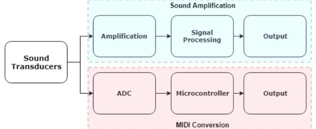
This section will take a more detailed overview of what has been done to make a MIDI adaptation and amplification of a harp by several harp makers. Following, there will be an individual approach to each topic of the project using as a guide the diagram in Figure 4.
Figure 4: Overview of the Problem
2.1
Approach Comparison
2.1.1 MIDI Conversion
As of today there are three main MIDI capable harpmakers/companies: Camac [1], David Kortier Harpmaker [3] and Glen Mountain Harps [4]. All of these examples use a similar approach with individual piezoelectric transducers placed at the bottom of the string making the conversion to MIDI through an internal circuit. Considering the celtic harp, only Mountain Glen has made full adaptations to MIDI, with the harp remaining capable of being used in a regular way.
In order to illustrate Figure 5 and Figure 6 show the comparison between a harp capable and not, respectively, of being used in a regular way (without amplification), with the biggest difference being on the size of the belly.
Figure 5: MIDI implementation on a regular harp
Figure 6: MIDI implementation on a non regular harp
For both Celtic and Pedal harps, these are only sold as MIDI or sound amplifi-cation harps and are individually made or adapted from pre-existing harps. In the website [4] some specifications are given stating the system provides both MIDI ON and OFF (informing when a note starts and stops vibrating) with the respective veloc-ity. Also, for further reference while developing, it is advertised that the total sampling and acquisition time is 8 milliseconds assuming a typical harp with 45 strings, even though not directly stated.
The Kortier MIDI system is sold in separate for non regular harps or adapted to pre-existing harps. No specifications are given in detail but from a previous personal experiences they only provide a MIDI ON information even though this characteristic may have changed in more recent harps. Details regarding the meaning of these MIDI message will be explained in more detail in chapter 2.2.2.
Some adaptations have been done by other private companies using the separate Kortier system however most of them result in a poor quality due to poor tuning or lack of understanding of the implemented system. The Camac version, as it is not available to the general public, does not provide many information about its adaptation with only live performances available.
Regarding Pedal harps it is not clear for any of them if the pedal mechanism makes any influence in the MIDI adaptation, which should result in a pitch variation. For Kortier and Mountain Glen Harps the resulting price of the MIDI adaptation alone can vary from 3,000$ to 5,000$, not including the harp.
2.1.2 Sound Amplification
Sound amplification capable harps, or more generally called electroacoustic harps, are much more common nowadays. Several companies such as Glen Mountain Harps [4], Camac [1], David Kortier Harpmaker [3] and Salvi [2] have presented versions of electroacoustic harps. Likewise, all the companies mentioned before sell both Pedal and Celtic electroacoustic harps. As a note, in the beginning of the 2010 approaches varied from microphone to piezoelectric however, today, all companies use a variation of the piezo pick-up placed at the bottom of the string.
As mentioned in section 1.2 there are no harps announced which implement both MIDI and sound amplification using piezoelectric transducers. The reason for that is not mentioned in any company as the mechanism as been proven useful for both implementations. Besides, it is clearly mentioned in the Kortier and Glen Mountain websites that MIDI harps do not implement the amplification system as of today.
For all the systems mentioned the amplification is usually done by some passive filtering on the piezo which is then connected to an already made pre-amplifier from companies such as Fishman [5]. This implementation can be seen in Kortier and Salvi harps, for example, however due to the pre-amplifier not being made specifically for the intended use the results can vary in quality.
2.2
Fundamentals
2.2.1 Sound Transducers
The sound transducer is the most important part of the whole project as it makes the conversion of the sound characteristics. One of the possible approaches to convert the vibration of the string into an analogue signal is the piezoelectric transducer ele-ment, mentioned from now on as piezo for shortening. As very well explained in The Principles of Piezoelectric accelerometers [6] piezo materials consist of active electrical ele-ments that produce an electrical output when excited by a varying force. They’re usu-ally made of a ceramic element, such as quartz, which possesses a crystalline structure. This structure, when submitted to a mechanical force will respond with a voltage pro-portional to the acceleration applied to it. In Figure 7 [7] it is observable the behaviour of a piezo element under different conditions with the respective voltage response.
Figure 7: Piezo voltage response to an applied voltage or mechanical force
This voltage occurs as the electrons inside the crystalline structure redistribute themselves when a force is applied and, if connected to a closing circuit, even leave the crystalline structure thus creating room for new electrons to enter the crystal. This movement generates an electromotive force that will stimulate charges to move around a circuit or within the piezo. The opposite can happen as well as by submitting the piezo material to an electrical field it will cause the crystalline structure to deform and generate a proportional physical force.
The piezo material can be, and has been, studied in many details however for this project only its electrical response is required for a good appliance. Without going into much detail, for the piezo element to properly work it needs a polling treatment. Usually a non treated piezo element will have dipole moments within its crystalline structured oriented in almost random directions. The treatment usually consists of placing electrodes to the surface of the piezo and applying a high DC voltage. After the treatment the piezo material will be polarized in the direction of the applied DC voltage and contain dipole moments fixed into a permanent configuration. This allows the behaviour of the piezo to be predictable when applying a force in a specific direction.
Ideally, as shown in Figure 7 a force applied in the polarization direction will re-sult in a positive voltage while a force applied against the polarization direction will result in a negative voltage. The polarization direction is very important as forces sub-mitted to the piezo in different directions will result in different behaviours, even when applied outside the polarization direction. A complementing explanation of piezoelec-tricity especially in regards to its fabrication materials and procedure can be found in the book Piezoelectric Sensorics [8].
In order to use the piezoelectric within a circuit a stable model needs to be im-plemented. As stated above, a piezo material will convert mechanical stress into an electrical charge. This relationship is named piezoelectric charge constant and is defined by the constant d which can be expressed in Coulombs (charge) per Newton (force) (1). This constant is associated with each piezo and varies with the direction of the applied force, always referencing to the polarization direction.
d = Q F I = dQ dt V = 1 C Z I dt= 1 C Z dQ dt dt = Q C (1)
Due to the lack of "charge sources" it is possible to make the conversion between charge and current using the formula in (1). As currents only varies when there is a variance in charge and the charge within a piezo is never constant when generating a voltage making the conversion to a current source gives a good approximation of its behaviour.
As an example, if a force is applied to a piezo and remains constant the piezo will produce a voltage until the equivalent opposing force of the piezo becomes the same value as the initial one. When this happens the piezo will no longer produce any volt-age as there is no varying charge. Furthermore, until now voltvolt-age has been mentioned even though the circuit has been translated as current source. Usually the piezo ele-ment is connected to the circuit using two electrodes in each side as displayed in Figure 8 which forms a capacitor behaviour. This capacitor in parallel with the current source will generate a voltage behaviour presented in formula (1).
Figure 8: Capacitive behaviour of a Piezo Element
This model is almost ideal for transient and dynamic applications but a more ac-curate representation also needs to account for the discharging of the piezo through current leakage, which can be represented by a parallel resistor. The final model is represented in Figure 9.
Figure 9: Equivalent Piezo circuit model
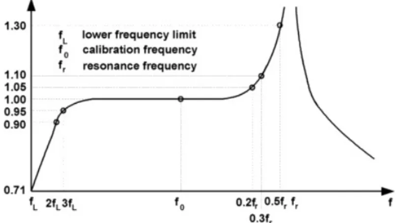
Regarding frequency response piezo elements have the typical frequency response of an high-pass filter with a resonance frequency. The behaviour is ilustrated in Figure
Figure 10: Frequency response of a piezo element
The values shown in Figure 10 are typical values for a piezo however these charac-teristics may vary a lot, especially for custom made piezos. Usually, piezos are defined by its resonance frequency. When using the piezo as a sensor this frequency should be as high as possible which allows sensors to work near the calibration frequency and provide more accurate and stable results as the gain should be 1. The resonance fre-quency coincides with the spot where the impedance of the piezo will be the lowest as possible. A typical piezo impedance curve is shown in Figure 11. The lowest peak rep-resents the resonance frequency while the highest peak reprep-resents the anti-resonance frequency, where impedance takes its highest value.
Some circuits, such as piezo quartz crystals oscillators, make use of this resonance frequency to oscillate at a precise frequency where the impedance is the lowest as pos-sible. This kind of circuits behave differently from the ones in study and cannot be represented by the model presented in Figure 9. Ideally for this project, the resonance frequency will be as high as possible and the lower frequency limit as low possible guaranteeing a wide bandwidth to work. As a note, the working bandwidth can be a little extended using a low pass filter with a cut-off frequency near the resonance frequency but this can only attenuate the resonance frequency.
The frequency response described before can be suitably modeled by equation (2). This equation shows the relation between the gain output (Go) relative to the reference
gain Gr (where ff
R = 1) and the input frequency f relative to its resonance frequency fR. The Q value, not to mistake with charge as described above, or quality factor,
rep-resents the "sharpness of the resonance" for each given piezo. Basically it defines how sharp, or wide, its resonance peak is. The higher the value, the sharpest the resonance frequency but also the higher the equivalent output gain.
Go Gr = q 1 (1− (ff R) 2)2+ 1 Q2( f fR) 2 phase lag (o) ≈ 60 Q f fR, f or f fR ≤ 2 5 (2)
The phase lag, which determines the lag in phase since the signal is applied until it is seen at the output, is also represented in equation (2). However, the phase lag is only relevant for high frequencies and for inputs that cross the piezo. Since the piezo will originate all the signals to be process phase lag will not have much, if any, impact in the project.
As stated before, the circuit should behave outside the resonance frequency how-ever it is possible for some piezos, especially low quality piezos, to have low resonance frequencies. This means that even if the string applied to a piezo contains a funda-mental frequency below the resonance frequency its harmonics, or overtones, may be beyond that point and get further amplified. Not only these frequencies get propor-tionately amplified as they may generate larger voltages than the circuit can handle.
As stated, this effect could be mitigated using a low pass filter but there is a trade-off between attenuating harmonics as they are the very essence of each instrument and serve to characterize its unique sound. This serves a note for later take into account during the development phase of the project.
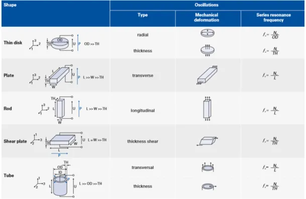
Also, if not indicated by the manufacturer, according to the company PiMicos guide [10] it’s possible to extrapolate the piezo series resonance frequency as exposed in Figure 12 by direction of applied force and dimensions of the piezo. This series res-onance frequency is a good approximation of the resres-onance frequency. This could be particularly useful for more undifferentiated piezos.
2.2.2 MIDI Conversion
To convert the output of the piezo into an electrical signal an ADC needs to be implemented. Most single board micro controllers such as the Arduino, which contains the ATMEGA328P [11] chip, or the most recently developed Teensy with a Cortex -R
M4-based micro controller [12] made specially for music applications, have embedded ADCs to convert the analog signal into a digital one.
Depending on the output of the piezo the signal may need some amplification and some filtering, such as a band pass filter, in order to present a readable signal for the ADC. This signal is usually contained within a voltage range and presents a maximum output impedance associated. An external ADC could be implemented but documentation of both microcontroller’s ADC have proved them effective to fulfil the need. Another advantage of using a microcontroller is the possibility of converting the ADC output to a MIDI message using the same device which reduces the overall area of the circuit and general latency. Using a single ADC for each piezo could prove effortless as not all the strings in the harp are being plucked at the same time.
A typical and simplified output signal of the piezo is represented in Figure 13. Al-though this response varies from instrument to instrument (and from type of string to string) and even from each piezo a common feature among all are the peaks associated with the decaying velocity of the string. By measuring the first peak, it is possible to ex-trapolate the force with which the string was plucked in the first time. Afterwards, by measuring each subsequent peak it is possible to make an assumption of the evolution of the velocity of the string after being plucked.
Ideally, if the string goes above a threshold a MIDI ON message will be sent with the corresponding velocity associated to the peak. As the signal decreases in ampli-tude, if the signal goes below a certain threshold a MIDI OFF message is sent. If the player stops the strings while its vibrating the behaviour should also be translated into a MIDI OFF message. All these messages will follow the standard MIDI protocol [13] which allows for the communication between instruments. As a curiosity, while this project is being developed MIDI 2.0 was announced bringing some new features, even though its basic operations remain almost identical. However, this project will focus more on having a good interoperability more than state of the art technology, for now. An example of a MIDI message is represented in Figure 15. To inform the com-puter that a note was played the algorithm will send three distinct message. The first, the Status Byte, will inform that a Note will be sent together with the corresponding channel, (the channel is a similar to an IP address when several computers are con-nected in the same network); afterwards, the Data Byte 1, which will inform exactly which note was played within a 127 possible range; lastly the Data Byte 2 will inform of the velocity associated with the corresponding note, also a value between 0 and 127. A MIDI OFF message would contain all this information with the Data Byte 2 set to 0.
Figure 15: Example of a MIDI message
At the output a typical MIDI output socket or USB connection can serve as a bridge to connect to other instruments or MIDI capable devices..
It is important to mention that a good MIDI conversion has a general latency of ~5ms with a maximum delay of ~10ms. A reasonable conversion should not only give accurate results but also give them within a time window.
2.2.3 Sound Amplification
Regarding amplification of the piezo there are several already developed pre-amplifiers for many different applications. Regarding audio these usually vary con-sidering the instrument or audio input that needs to be amplified. Nonetheless, the majority are usually pretty expensive and most importantly, are not developed for the specific instrument. For a guitar or piano it is possible to find a unique developed circuit however outside of this scenario it becomes rather difficult.
In this project since there will be several piezo inputs there is a need for a simple amplifier solution for each individual piezo. Further on, after this first stage amplifica-tion, the sound can be individually filtered and the sum of all the signals can be driven through a common filtering process and final tunable gain. This approach allows for a more precise tuning of each single piezo in the first stage amplification followed by a final tuning of the sum of all the signals in a second stage amplification.
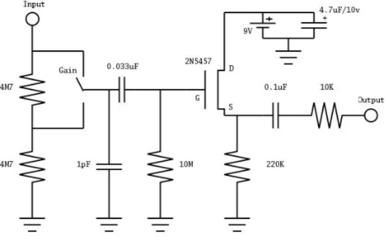
Regarding the first stage many circuits have been published and proposed to am-plify a piezo signal. A very simplistic approach, found in a DIY (Do it Yourself [14]) project can be found in Figure 16. This design consists of a very basic voltage divider, used to control the voltage output of the piezo, which could be replaced by a poten-tiometer for more accurate tuning, a high pass filter, in order to remove noise and interference, and finally a single Jfet to amplify the sound. At the output of the Jfet the the capacitor and resistor serve to remove any DC signal and bring everything to a typical line level. The values for each component should be designed according to the specific piezo in use.
Figure 16: First Stage Amplification Example
For the second stage a simple application using an op-amp might be the best choice with a tunable filter for a more accurate approach. A design made for 5 channels is available in [15]. Despite all of these approaches it is most important to first study the response of the piezo and then build the system around it.
Also, while using piezos the most important feature is to match the output impedance of the piezo with the input impedance of the amplifier. A mismatch between these two devices can really affect the sound output, leading to inconsistent or very attenuated gains. It is also important to consider leakage current in order to minimize the circuit power consumption.
As a conclusion, ideally, it is important to keep a maximum voltage and signal quality the closest to the amplifier mechanism as it is easier to make tunings regard-ing audio when convertregard-ing from higher to lower voltages than the opposite. Keepregard-ing minimal distortions while still conditioning the signal to an audio output is the main objective for the audio implementation. To verify these parameters, even though de-signed specifically for mosfets, a very well written guide regarding testing can be seen in [16].
3
Inital Approach
In this section an initial approach to the project will be described together with the discrete objectives the project will aim to fulfil. This section will not go into much detail regarding deployment of the implementation as that will heavily depend on experimentation and testing. It will serve more as a guide to develop the rest of the project.
3.1
Discrete Objectives
In order to verify and validate the project some objectives need to be defined. These are:
Main Objectives
• The transducers need to capture the vibration of a string of an harp and convert it to an electrical signal;
• The MIDI circuit, using a micro controller, must be able to convert the signal from the transducers into a MIDI message;
• The transducers must allow the musician to play without disturbing regular use of an harp;
• Player controllability of the circuit should be maximized;
• The MIDI conversion should be done within the normal latency requirements: maximum 10 ms, optimal should be around 5ms;
For this project the MIDI implementation serves as the main driver and the ampli-fication module serves as a secondary driver. If possible both should work using the same piezo and possibly work at the same time. However if not possible there should be a switch to toggle the piezo to be amplified or converted to MIDI.
If time and cost are of no restriction the amplification module should be imple-mented with the following objectives:
Secondary Objectives
• The amplification module must allow for the direct connection of a regular am-plifier;
• The amplification module should not condition any of the main objectives; • The amplification must allow to be controlled and, if possible, tuned by the player.
3.2
Initial Methods
The first approach to the project will be comparing several piezo types regarding signal and frequency response. In order to achieve that a small structure will be used which can fixate strings and place piezo elements at its base, such as a guitar or ukulele. This will serve to build an initial database with each piezo characteristics. Until now the company PI Ceramics [17] has been contacted and supplied two samples of piezos for testing during the development phase. Besides, several typical piezo disks have been bought to test and compare.
Further on, a basic program will be implemented to convert the signal of the piezo using a Teensy or Arduino board. Together with a virtual oscilloscope this will allow to collect samples and retain them for comparison. This is important as signals collected from an actual oscilloscope and ADC can radically vary due to the internal resistance of the ADC, however this topic will be studied in more detail in section 7.2.2. After validating the piezo the MIDI module will be implemented according to the Main Ob-jectives defined in section 3.1
After the MIDI module is finalized and validated, testing with the amplification module will start by using each developed piezo in an embedded amplification circuit. This will require isolation between the two mechanisms not to cause any interference with each other. As stated in 2.2.3 an initial stage amplification will be built for each individual piezo and its results validated. Finally, several outputs will be summed and
Once the validation and testing of both mechanism proves functional a small anal-ysis on the overall benefits and place on the market will be discussed an taken into consideration. This is an important step since this project has the goal of creating an innovative project within the harp and music subject.
4
Work Methodology
This section will contain a very brief description of all the tools planned and used during the preparation and development phase of the project. It will as well contain a work schedule procedure for the development of the project.
4.1
Project Phases
The project will consist of two distinct phases, the preparation phase and the
development phase. The preparation phase will be executed prior to the beginning of the project. The development phase will start near the end of the first phase will be continued until the final delivery of the project.
4.1.1 Preparation Phase
The preparation phase consisted in following by order of the presented topics: • Investigation of the different approaches to convert sound to MIDI; • Investigation of approaches to amplify sound using sound transducers; • Matching of the two previous topics in one single implementation; • Market study of the different components;
• Ordering of the components to be used in the Developing phase; • Study of the tools to be used during the Developing Phase.
All of these topics have in parallel a continuous gathering of information from specialists within and outside the academic environment.
4.1.2 Developing Phase
The Developing phase will consist in following by order the presented topics:
• Weeks 1-5 Conclusion and validation of all the information gathered during the Preparation phase
• Weeks 2-5 Initial Testing and implementation of the pre-schematics
• Weeks 3-5 Validation of the pre-schematics in accordance to the main objectives • Weeks 6-8 Implementation of the studied systems and second ordering of
com-ponents
• Weeks 9-10 Tuning and cleaning of noise within the implemented circuit • Weeks 11-12 Implementation of the MIDI Algorithm
• Weeks 13 Validation of the algorithm
• Weeks 14-16 Final Verification and Validation of the implemented schematics • Weeks 17-18 Preparation and Writing of the Dissertation
All of these topics have been continuously evaluated by the supervisor and sub-mitted to approval and/or changes when requested.
4.2
Project Tools
For this project the following tools will be used in order to fulfil objectives: • Oscilloscope To gather data from the circuit at any given point
• Python: matplotlib In order to simulate and gather data and graphics from the oscilloscope
• National Instruments Multisim In order to simulate the behaviour of the circuit and piezos
• Micro Controllers: Arduino, Teensy To read and process data from any given piezo or input
• Electrical Components To build the circuit in need
5
Research Methods and Developed Tools
This section contains a description of the used and developed tools to validate the system.
5.1
Research Tools
5.1.1 Oscilloscope
The oscilloscope in use will be DSO10112B [18]. It has 4 analog channels capable of sampling at 1GSa/s each, a 100MHzprocessor clock speed and a 2 mV/div per 2 ns/div
minimum resolution. Since the measured signals should not have an amplitude below 10 mV and 20 Hzthis specifications should suffice. It is also capable of performing Fast
Fourier Transforms which will be particularly useful during the audio amplification development and will be explained more in detail in 5.2.4. The probes in use contain a high impedance of 1MΩ and a small capacitance of 5 pF.
5.1.2 Multisim
In order to simulate the circuit behaviour the NImultisim software [19] will be used. This tool will be most usefull during the dimensioning of the audio amplification circuit specifically for filter designing. However, due to the characteristics of the piezo it is very challenging to accurately replicate its behaviour in a simulation and plan accordingly. The signal amplitude will vary in time, frequency will change in phase and the peak resulting from physically plucking the string will affect all the remaining signal.
For that reason the multisim tool will only be used as a theoretical help to imple-ment and predict frequency response of the amplification signal more than an accurate estimation of the expected result.
5.1.3 Developed Software
In order to validate the results from the microcontroller it is important to visu-alize the inputs coming from the piezo signal using the internal ADC, in opposition to the oscilloscope. For that, the Arduino IDE already provides a tool to visualize the signal however, this tool, as it stands, is only capable of visualizing 300 samples with no control over its window or number of inputs on screen. To fix this issue a pro-gram was developed from the ground up allowing to visualize any samples coming from the Teensy microcontroller, or any other board, in real-time using a program in python available in [20]. As it stands the program is capable of: visualizing the signal in real-time; visualizing up to 8 concurrent signals; stop the image and zoom in/out in any location; work in continuous mode or trigger after a certain event; define any maximum voltage or bit resolution for the signal.
Furthermore, the program is also capable of displaying the x values in numerical samples or associated timing. Yet, this last option introduces a small delay while pro-cessing which delays the whole signal per sample. This is an issue that will be fixed in future versions explaining why the figures from this program will be displayed us-ing a sample based X-axis. Also, the program shows the average delay since sendus-ing the sample until it is processed on top of the window which could give an idea of the sampling rate time and adjust the intrinsic per-sample delay.
Finally, a second program was developed on top of the previous one to visualize the incoming signal in the frequency domain also available in [20]. This program is only capable of processing one input as it stands and it is available in [fft_git_me]. It is possible to define several windowing methods as well as number of samples to collect until the FFT is processed. This program should serve as a tool to help validate the signal coming from the oscilloscope.
5.2
Teensy Microcontroller
5.2.1 Characteristics
For this project, as stated in section 4.2 a Teensy 3.5 development board [21] will be used. This board contains a 120MHz ARM Cortex-M4 microprocessor[12] together with 512K Flash memory and 192K Ram memory. It contains 62 I/O pins available from which 26 pins support analog signals up to 3.3 Volts. As a note it is possible to overclock the microprocessor up to 168 MHzif needed however, this is not recommend
for long periods of time as it shortens the life expectancy of the microcontroller.
Besides the ample number of I/O ports the Teensy board was chosen due to its specific development towards sound processing. It contains embedded audio codecs, capable of encoding and decoding audio files from an SD Card, 14 independent hard-ware timers and most important 2 dedicated ADC’s capable of working independently of each other.
These are not all the specifications regarding the Teensy 3.5 but a sum of the most useful ones regarding this project. Finally, the Teensy 3.5 was chosen instead of the model 3.6, which would have a higher clock speed of 180MHz, due to its 5 Volt toler-ance in the I/O despite only working up to 3.3 Volts. This characteristic can be quite important while testing and even in the final product as piezo elements can behave er-ratically when submitted to unpredictable pressure or heat. It allows for a more robust implementation both while testing and as a final product.
5.2.2 Teensy and Python oscilloscope - Validation of a Single ADC
One of the central aspects of this project is the ADC capability of the Teensy board. Even though the oscilloscope described in 5.1.1 is more than capable of analysing the signal from the piezo it is very important to keep in mind that the embedded ADC will have a much lower signal accuracy and sampling speed when compared to the oscilloscope. This means that signal characteristics displayed on the oscilloscope can be lost to the microcontroller’s ADC if, as an example, the signal changes too fast or
Besides, the teensy’s ADC contains an internal capacitance of 5pF and most im-portant an internal impedance of 2 kΩ. This means that signals collected in the oscil-loscope, due to its 1MΩ will have a much higher voltage than signals collected inside the Teensy. This difference increases the higher the voltage and output impedance of the whole circuit load before the ADC input.
First, in order to test accuracy, the ADC will be submitted to a 5kHz signal
pro-vided by a signal generator, using a very low output impedance of 8Ω as recommended by the microcontroller datasheet. This frequency serves to guarantee that most signals from the piezo will be captured since their frequency should be mostly below 2kHz.
The microcontroller will contain a program which will collect 2000 samples to a buffer and afterwards print them out to the Serial Interface. To control the ADC characteristics the official ADC library, available in [22], will be used. This library allows a straightfor-ward control of the sampling speed (how fast samples are collected), bit resolution up to 16 bits (how many discrete intervals between 0 and 3.3 Volts) and conversion speed (how accurate the voltage signal is converted to a discrete value). After executing, the program will also display how much time collecting the samples and sending them took.
The Serial Interface will be connected to a computer which will run a program in Python. This program was developed from the ground up and it is available in [github_python]. The program will receive the samples from the microcontroller and display in real-time a graph illustrating its results. At the same time the program will calculate the average delay between samples which allows to estimate the total and single send delay from the computer side.
The results are illustrated in Annex A table 5. It is possible to observe that, as ex-pected, the higher the conversion and sampling speed the faster the signal is obtained, with the total time to collect 2000 samples going from about 6 ms to 27 ms which is a very significant. Changing from 10 bits to 16 bits resolution affects time consumption with an increase of 10% to 20% the faster the conversion and sampling speed. It is ob-servable that the faster the samples are collected the closer values from 12 bit and 16 bit get to each other.
Regarding signal send time, as expected, this value is independent of sampling collection and only varies from bit resolution, taking about 5 µs per sample. These times remain fairly constant as they do not depend on the ADC characteristics but rather on the information size and bit change. As an example, using 4 bits to send the number 0 (in binary: 0000) or 15 (in binary: 1111) takes less time than sending the number 10 (in binary: 1010) due to the increase in bit change. This justifies why processing times are exponentially varying the higher the bit resolution. There is also a delay between sending and receiving values of about 3 to 4 µs. This delay may be due to the python program generating a graph at the same time however, this is not a very relevant variable as only MIDI messages will be sent to the computer and not constant data.
Regarding sample quality, also in Annex A in Figure 74d tests B, E and I are il-lustrated for both 10 and 16 bits resolution. The results show only 500 samples for better signal analysis. By observing the results it is perceptible that as the sampling speed increases less signal periods are captured as more information is collected about each individual period. However, even when comparing a slower test to the fastest test there is no decrease in sample quality with no typical glitches present. Also, by comparing both 10 and 16 bits, side to side, there is no observable variation in quality whatsoever even for the fastest test implemented.
The same tests where implemented using a wave with the same frequency but with an amplitude of 50 milivolts peak-to-peak. A 10 bit implementation is able to detect a maximum of 3 milivolt variation while a 16 bit implement can detect up to 50 microvolt variation. However this limit is not usually imposed by the bit resolution but by the intrinsic ADC accuracy during its conversion. By looking at Figures 73a through 73f the existence of glitches becomes very noticeable increasing the faster the test is performed and the higher the bit resolution gets. For the slowest test shown at 10 bits the worst variation is 10mV with an average of 3mV error while for the fastest test at 16 bits the worst variation is 13mV with an average of 6mV error. This means that in order to detect smaller variances an averaging may be needed to decrease these kind of errors.
Finally, a final program was implemented using interrupts to generate ADC read-ings. After several attempts for collecting samples this method revealed the fastest and most accurate. The process consists of a timer generating an interrupt at a defined pe-riod. This timer when activated will generate a pulse in a digital output and start an ADC reading. When finished, the ADC will generate an interrupt, collect the value and generate a pulse. The difference between these two pulses reveals the timing the ADC takes to read a sample and can be measured in an oscilloscope. An example of a signal can be seen in Figure 17. The results for each test at both 12 and 16 bits are represented in Annex A in tables 7 and 8.
Figure 17: Example of the timing window for Medium Sampling and Conversion Speed at 12 bits
These tables serve more as reference point for later implementations of the signal sampling. As expected, the timings follow the same pattern as already discussed for table 5. Finally, some measurements were done using different averaging which are represented in Annex A in table 9. However, varying in averaging only multiplies the samples taken each time. After a certain amount averaging follows a linear pattern.
As a final conclusion, it is proved that it is possible to execute the ADC at higher speeds with the highest resolution. If changes below 10 milivolts need to be obtained, at 16 bits, some averaging may be needed to apply. Regarding the serial interface, since no signals will be sent consecutively as in this example but only single MIDI messages the teensy development board is more than capable of executing the requirements im-posed in 3.1.
5.2.3 Teensy and Python oscilloscope - Validation of a Both ADCs
In section 5.2.2, each ADC was validated independently. For this project both ADCs will be used at the same while connecting to several inputs each. Due to the configuration process one ADC can only be linked to an input at each time. This means that for reading several inputs at the same time the ADC configuration needs to be changed on the fly while capturing data.
Figure 74, presented in annex A, shows four tests done in order to compare the delay between acquiring one and two inputs in each ADC. The tests were run using the fastest settings at 16 bits for 500 samples. By looking at table 6 it is noticeable that both ADCs working at the same time for a single input will take the same amount of time as a single ADC working for a single input. However by imposing a switching mechanism between two inputs for one ADC the time goes up about 2.1 times.
This means that the switching mechanism alone takes about 5% the time of col-lecting a sample at the fastest settings. Also by looking at Figure 74d in which one ADC is oscillating between two inputs and the other is reading a single one this delay becomes visibly noticeable by the number of periods acquired. This alone is not that problematic however when scaling for 3, 4 or more inputs at the same time in one ADC it can generate significant delays.
This is unfortunately expected and it is important to keep this detail in mind while developing and escalating the MIDI circuit for several inputs. However, for the MIDI implementation as long as the peak is collected there should be no problem in this regard. Apart from this no quality degradation is observed throughout the test.
5.2.4 Teensy and Python Fast Fourier Transform
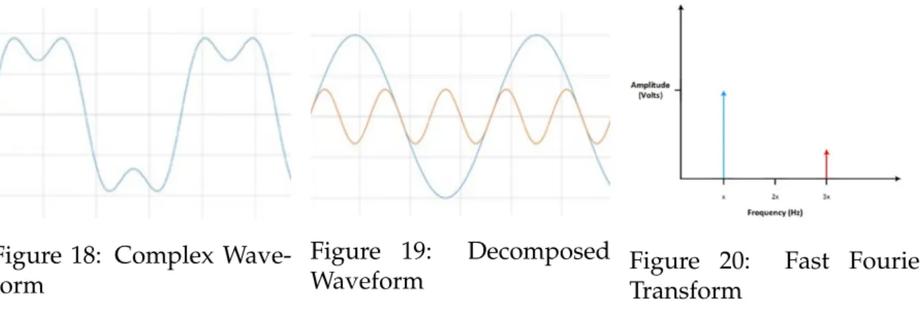
In order to validate the piezo itself as well as the audio amplification side, it is important to verify its frequency response. The ideal way is to use a FT (Fourier Trans-form) which converts a signal from its time domain to its frequency domain. The result of a FT should be in a graph displayed with frequency per voltage (or dB) in amplitude. Ideally, the result of a perfect sinusoidal wave is displayed through a single peak in its frequency with the corresponding voltage amplitude. Even more complex waves can be decomposed into a sum of sinusoidal waves which can therefore be represented by single peaks, as shown in Figures 18, 19, 20.
Figure 18: Complex Wave-form
Figure 19: Decomposed
Waveform Figure 20:Transform Fast Fourier
For a digital circuit to perform a Fourier transform the solution is to implement a DFT (Discrete Fourier Transform) that applies the same principles but for discrete data sets which display the result in discrete frequency bins. These bins represent a set of frequencies in which the signal is contained and can vary in size depending on the sampling rate of the signal and windowing applied. In this case the FFT (Fast Fourier Transform) will be applied as its an optimized version of the DFT, to reduce computation time.
Also, when sampling a signal, usually the data is not contained within perfect boundaries. In other words, each individual signal, resulted from the decomposed wave, does not start and end at the beginning of a period. Because of this, the DFT result will show high frequency components not present in the original signal. Be-sides, since the original signal is always windowed prior to the FFT transformation,
the magnitude spectrum will present leakage to near frequencies. This makes the re-sult look more as a curve more than an impulse. This effect is called spectral leakage as is represented in Figure 21.
To mitigate this effect a windowing technique mentioned before can be applied. Windowing mainly aims to reduce the effect of the high frequency components but can substantially reduce spectral leakage. This is achieved by multiplying the finite set of data with a curve which gradually smooths the edges of the data towards zero approximating the starting and ending value of the waveform. A representation of this effect is demonstrated in Figure 22.
Applying a window is not as trivial and can change the result drastically depend-ing on which technique implemented as well as the original signal. Windowdepend-ing tech-niques are well beyond the scope of this project, however a good and more detailed explanation windowing and spectral analysis in general is Spectral Audio Signal Pro-cessing by Julius O. Smith [23].
Figure 21: Spectral Leakage without windowing
Figure 22: Spectral Leakage with win-dowing
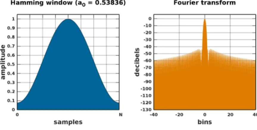
There are several types of windowing techniques that can be applied with the most common ones being Rectangle (no Window), Hamming and Blackman, with many variants even within these last two. Typically the Hamming window will fit 95% of the scenarios however, for most audio applications the Blackman window technique is the best one to apply. A comparison between the Hamming and Blackman window technique can be seen in Figures 23 and 24.
Figure 23: Hamming Windowing
Figure 24: Blackman-Harris Windowing
This Blackman method aims to minimize frequency leakage which is rather impor-tant for this project: as the string vibrates the main frequency leakage can attenuate the harmonics produced by the string hiding its effect. However, this method widens the frequency bins to achieve this, leading to less frequency accuracy, and removes power
However, for this application, frequency accuracy is not a big concern as the ex-pected main and harmonics frequency are known from the string tuning. Also, even though there is a power attenuation in the signal the proportion between the frequency peaks is maintained leading to a relevant analysis at the end. By testing several varia-tions of the Blackman windowing the Blackman-Harris variation is the most accurate representation of all.
As the oscilloscope mentioned in 5.1.1 does not possess the Blackman-Harris vari-ation windowing one had to be implemented in the Teensy using the official audio library [24] together with the ADC library [22]. The Teensy will collect several samples and perform an FFT using the Blackman-Harris windowing. Afterwards, it will send the signal through the Serial Interface allowing the already mentioned Python program to display the graph.
It is important to mention that in order to collect samples using the Teensy the signal needs to be within the 0 to 3.3 volts margin. In some cases this can be applied, however, in many of them an oscilloscope needs to be used.
6
Piezoelectric Transducer
This section contains all the details and decision process regarding the piezo ma-terial and its design.
6.1
Concept and Initial Design
The initial approach for choosing the ideal piezo for this project was both to con-tact piezoelectric elements manufacturers and research piezo elements used to amplify acoustic guitars, which are the most common. The second option presented no results as guitar companies do not reveal which types of piezo elements are used. Also, many DIY (Do it Yourself) projects had information regarding piezo disks which are not ideal to be added directly right under each string. The first option resulted in the company Pi miCos [10] recommending the PIC255-0753 piezo element. This number informs that the piezo is made of the material PIC255, a modified lead zirconate-lead titanate, with the company reference number 0753 to specify dimensions of 5x2x0.5 mm (LxWxH).
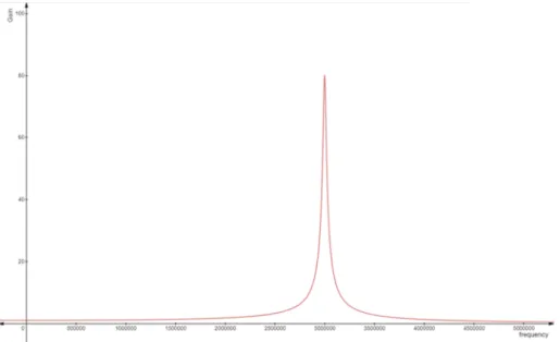
This cuboid piezo seems ideal for the project due to its small dimensions and datasheet characteristics which specify a high piezoelectric charge constant (already described in section 2.2.1) of about 550 pC/N, a maximum of 100 Vpp Voltage re-sponse, and a resonance frequency of 3MHz. The quality factor constant Q is stated
as 80. By using equation 2 presented in section 2.2.1 the curve displayed in Figure 25 is obtained.
Figure 25: Frequency Response of Piezo PIC 255-0753
Reminding Figure 10 in section 2.2.1, this high resonance frequency gives a high bandwidth window to work within. Only frequencies above 2MHz should
demon-strate an average gain which is well beyond the working window established.
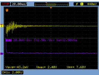
However, in order to get the electric signal two ways can be used: by soldering the piezo element, which requires special ovens that prevent changes in the internal char-acteristics to change their orientation by using low temperature and a special solder, not available; by using contact metal pieces attached to both sides of the piezo.
This last solution was applied using several types of conductive materials and pressure points on the piezo. However, the best results obtained are presented in Fig-ure 26. This FigFig-ure displays both the output signal (in yellow) and the associated FFT (in purple). Neither display a significant result for the applied frequency of 348Hz
Figure 26: Results of the Cuboid Piezo element using metal contact
Since no signal can be captured from the initial piezo another possibility is to cap-ture the signal from another piezo while attaching the first piezo to it. This would mainly maintain the characteristics of the initial piezo, denominated from now on as piezo_A, while using the second to conduct the electric signal, denominated as piezo_B. Assuming piezo_B has a weaker nature (regarding piezoelectric charge con-stant and voltage response) there shouldn’t be much interference in the circuit. Such a piezo is easily available and consists of a piezo disk. The idea resulted in the schematic shown in Figure 27 and 28.
In the schematic piezo_A (1) is attached to piezo_B (2) which consists of a small disk. The string, in contact with the piezo_A (1) will oscillate producing a vibration which will pass to piezo_B. Piezo_B will remain on top of a hollow cylinder (3) al-lowing this oscillation to occur. The base support (4) will prevent any oscillation from below, such as the harp belly or near strings reverberation, to affect the piezo response.
In this case the cylinder (3) contains a gap allowing wires attached to piezo_B to pass, this could also be done from the base of the base support (4). The enclosure (5) serves only to protect the inside and provide an aesthetic improvement.
Figure 27: Side View of the Piezo Structure
Figure 28: Top View of the Piezo Structure
As the ideal piezo disk element was well past the limit budget, the closest to ideal piezo disk element obtained was the 7BB-12-9 and the 7BB-15-9 [25]. These two piezos vary in diameter, 12mm and 15mm respectively, and resonance frequency, 9kHz and
6kHzrespectively. The low resonance frequency can be a problem as frequencies near
1kHzand above can be extra amplified. This comes only as an estimation as no quality
factor is provided by the manufacturer. Regarding MIDI this will not be a problem however, for audio amplification, it can lead to more high frequency components. This effect can be more or less mitigated using a low pass filter if needed, which is a topic already discussed in 2.2.1.
6.2
Piezoelectric Disk Testing
In order to test the piezo disk individually the schematic shown in Figure 27 was assembled. The cuboid piezo element was replaced by a copper cuboid of the same size, the cylinder was made out of brass metal and the base support made out of rubber. The results of a medium force pluck can be seen in Figure 29 and 30 with the wave from the piezo represented in yellow and the FFT shown in purple. These results display a more promissing result with the respective FFT showing the fundamental frequency, F4 at 348 Hz, and three of its harmonics at 670Hz, 1047Hz and 1400Hz. These harmonics coincide with the expected as they are multiples of the fundamental frequency F4. Also, as the string is pressed and then released, stretching and compressing the piezo, a negative voltage peak occurs as expected due to the initial stretch of the piezo. As the
Figure 29: Piezo Result of medium pluck with FFT
Figure 30: Amplified Piezo Result of medium pluck with FFT
By doing the same test with a stronger pluck of the string the results shown in 31 are obtained. It is important to notice the increase in amplitude, from about 3.5 to 7.5 Volts, which is to be expect as more force is applied on to the piezo. The increase in the harmonics amplitude, comparing to the fundamental frequency, happens due to the low resonance frequency and is easily noticeable. This results implies a low quality factor of piezo_B as frequencies near 1kHz are further amplified than the fundamental
frequency.