Repositório ISCTE-IUL
Deposited in Repositório ISCTE-IUL:
2019-03-27Deposited version:
Post-printPeer-review status of attached file:
Peer-reviewedCitation for published item:
Ferreira-Lopes, A. (2010). In or Out? The Welfare Costs of EMU Membership. Economic Modelling . 27 (2), 585-594
Further information on publisher's website:
10.1016/j.econmod.2009.11.013Publisher's copyright statement:
This is the peer reviewed version of the following article: Ferreira-Lopes, A. (2010). In or Out? The Welfare Costs of EMU Membership. Economic Modelling . 27 (2), 585-594, which has been published in final form at https://dx.doi.org/10.1016/j.econmod.2009.11.013. This article may be used for non-commercial purposes in accordance with the Publisher's Terms and Conditions for self-archiving.
Use policy
Creative Commons CC BY 4.0
The full-text may be used and/or reproduced, and given to third parties in any format or medium, without prior permission or charge, for personal research or study, educational, or not-for-profit purposes provided that:
• a full bibliographic reference is made to the original source • a link is made to the metadata record in the Repository • the full-text is not changed in any way
The full-text must not be sold in any format or medium without the formal permission of the copyright holders. Serviços de Informação e Documentação, Instituto Universitário de Lisboa (ISCTE-IUL)
Av. das Forças Armadas, Edifício II, 1649-026 Lisboa Portugal Phone: +(351) 217 903 024 | e-mail: [email protected]
Membership
Alexandra Ferreira-Lopes
yAbstract
Sweden and the UK have repeatedly refused to join the European and Monetary Union (EMU). Surprisingly, there is very little work on the welfare consequences of the loss of monetary policy ‡exibility for these countries. This paper …lls this void by providing a framework to evaluate quantitatively the economic costs of joining the EMU. Using a two country dynamic general equilibrium model with sticky prices we investigate the economic implications of the loss of monetary policy ‡exibility associated with the EMU for each country. The main contribution of our general equilibrium approach is that we can evaluate the e¤ects of monetary pol-icy in terms of welfare. Our …ndings suggest that these economies may experience sizable welfare losses as a result of joining the EMU. Results show that the cost associated with the loss of the monetary policy ‡ex-ibility is higher in the presence of persistence government consumption shocks and small trade shares with the EMU.
JEL Classi…cation: C68, E52, F41.
Keywords: Monetary Policy, Euro, UK, Sweden.
The author would like to thank João F. Gomes, Álvaro Pina, Emanuel Leão, Ellen Mc-Grattan and Oliver Holtemöller, participants at the ASSET Annual Meeting of 2004, par-ticipants at the IX Dynamic Macroeconomics Workshop held in Vigo, parpar-ticipants of the Money and Finance Conference at ISEG, participants of the 9thAnnual Conference of SPIE
(Portuguese Society for Research in Economics), especially Ana Paula Ribeiro, participants at the 4thConference of the European Economics and Finance Society, participants at 22nd Symposium for Banking and Monetary Economics, especially Nina Leheyda, participants at the 20thConference of the European Economic Association, especially Zsolt Darvas,
partic-ipants at the Doctoral Seminars in Economics at ISEG and at ISCTE, particpartic-ipants at the 12th Conference of the Society for Computation in Economics and Finance, participants at
the 2ndGerman MacroWorkshop, participants at the New Developments in Macroeconomic
Modelling and Growth Dynamics Conference, participants at the 38th Money, Macro, and
Finance Conference held in York, and also to participants at the ASSET 2006 Conference in UCP, Lisbon, for helpful comments and suggestions. I am responsible for any errors or omissions.
yISCTE - Lisbon University Institute, Economics Department, Economics Research Center
(ERC)-UNIDE, and DINÂMIA. Avenida das Forças Armadas, 1649-026 Lisboa, Portugal. Tel.: +351 217903901; Fax: +351 217903933; e-mail: [email protected]
1
Introduction
Should UK and Sweden adopt the Euro? In this paper we construct a two country dynamic general equilibrium model with sticky prices to evaluate the economic costs of the loss of monetary policy due to joining the European and Monetary Union (EMU), for these two countries.1 Our focus is the loss of
auton-omy of monetary policy and its implications for business cycle synchronization. Business cycle synchronization is an important decision factor for joining the EMU. It is often argued that it is not a good decision to join the euro, if a coun-try’s economic cycle is not synchronized with that of other remaining members as a common monetary policy may actually accentuate economic ‡uctuations (for example Gros and Hefeker, 2002).
General equilibrium models with nominal rigidities have been used to study the problem of the loss of independence of monetary policy, usually using ex-tensions of the Obstfeld and Rogo¤ (1995) model. The referred model is used to compare between an autonomous monetary regime (multiple currencies and di¤erent monetary policies) and a monetary union. The model, in a two country framework, has been used to assess the consequences on individual welfare of the loss of exchange rate ‡exibility, when facing asymmetric shocks. Some con-clusions drawn for the French economy, …nd that in the presence of asymmetric permanent shocks to either technology or government expenditures, it is bene-…cial to households living in the country hit by an asymmetric shock to join a monetary union (Carré and Collard, 2003). Other conclusions state that entry is welfare improving the smaller the country, the smaller the correlation of tech-nological shocks between countries, the higher the variance of real exchange rate shocks, the larger the di¤erence between the volatility of technological shocks across member countries, and the larger the gain in potential output, compared with the gain in potential output of a ‡exible exchange rate regime (Ca’Zorzi
1Denmark is not analyzed, although it is one of the three former EU-15 countries that
did not join the European currency, because it has a exchange-rate peg to the euro, so the study of the e¤ects of loosing monetary policy independence does not seem relevant, since independence is already lost.
et al., 2005).
When used to study the costs in terms of stabilization and welfare of joining a currency union, the class of models mentioned in the paragraph above, reveals that countries face a trade-o¤ when joining a monetary union between higher instability in output and lower instability in in‡ation, and that this trade-o¤ im-proves with the degree of cross-country symmetry of supply and demand shocks. These results lead to the conclusion that maintaining the monetary stabiliza-tion possibility proves to be always welfare improving, independently of the changes in the correlation and type of shocks (Monacelli, 2000). Corsetti (2008) studies the costs, in theoretical terms, of loosing monetary policy independence and exchange rate ‡exibility in the light of optimum currency area theory, us-ing a micro-founded choice-theoretic model. The author states that a common monetary policy produces a level of economic activity which is lower than the optimum, but since exchanges rates do not present a stabilizing role as stated by the optimum currency area literature, monetary policy can be e¢ cient, if the proportion of national goods in the consumption basket of the union is similar to the share of value added in total GDP across countries.
Brigden and Nolan (2002) in the context of a new-keynesian model study the variability of a country’s output and in‡ation if it decides to join a monetary union. They …nd that the EMU increases the volatility of output and in‡ation and that loosing the ability to stabilize the domestic economy is less costly if supply shocks are small. They estimate that the UK stabilization cost for joining the EMU is equivalent to a permanent reduction in GDP of between 0.6% and 2%. Pesaran et al. (2007) are also concerned with the behaviour of output and in‡ation regarding the decision of the UK and Sweden of joining the EMU. They perform a counterfactual analysis using a global vector autoregression (VAR) model, to assess what would have happened if the two countries have joined the EMU in 1999. Results for the UK regarding di¤erences in output and in‡ation are small and change between the short and the long run, but are robust to various scenarios. Welfare results would be inconclusive, since output
and in‡ation behave in opposite directions, and of course, would depend on the relative importance of each variable. Results for Sweden are di¤erent from those of the UK, and since output and in‡ation would both increase, no robust conclusion about welfare is possible.
McAvinchey and McCausland (2007) used a macroeconomic framework to estimate empirically the impact on the UK economy of joining the EMU, par-ticularly concerning di¤erences in income and macroeconomic policies. The authors found evidence that macroeconomic policies and economic structures of the two zones share similar time paths to those which would happen if the UK was already in the EMU.
In this paper we develop a two country dynamic general equilibrium model with sticky prices, so that monetary policy can be used as a short run policy instrument of economic stabilization. We then investigate the economic impli-cations of the loss of monetary policy ‡exibility associated with the EMU for each of these countries. Speci…cally we consider two di¤erent scenarios: (1) one in which the country is currently inside the EMU and therefore the monetary policy rule is established by the European Central Bank (ECB), that follows a weighted Taylor Rule, designated Common Monetary Policy; (2) another where the country is outside the EMU and therefore the monetary policy is established by the country’s National Central Bank, that follows a Taylor Rule, designated Autonomous Monetary Policy. We then examine the macroeconomic implica-tions of these two policy arrangements and o¤er a detailed welfare analysis to formally assess which is preferred by domestic residents.
In order to do a welfare analysis to evaluate di¤erent monetary policy regimes, this work brings together two types of literature: the optimum currency areas literature with seminal work by Mundell (1961), McKinnon (1963), and Kenen (1969) and the dynamic stochastic general equilibrium models (DSGEM) liter-ature in the tradition of Obstfeld and Rogo¤ (1995) and Chari et al. (2002a).2
We use this framework to study the decision to join the European Monetary
2See Goodfriend and King (1997), Clarida et al. (1999), and Lane (2002) for surveys on
Union in terms of the loss of monetary policy ‡exibility for Sweden and the United Kingdom, calibrating models speci…cally for each economy; a task we have never seen done in the literature and for the purpose stated above.
We also introduce a new interest rate rule for the ECB, that ponders the Eurozone countries’s weights, since countries do not have the same economic weight and hence its economic condition will enter in the interest rule of the ECB with di¤erent weights. This modi…cation is important because a big country can in‡uence the way the interest rate rule moves if it enters the Eurozone, but a small country’s in‡uence is much smaller, hence business cycle synchronization becomes more important. Holtemöller (2007) calculated an optimum currency area (OCA) index to measure the economic consequences of joining the EMU and uses a Taylor Rule similar to the one we introduced here, but in a di¤erent economic framework and calibrating the model for the new member countries of the European Union. The OCA index measures the relative loss in terms of output gap and in‡ation variability in the two regimes stated above.
The outline of the paper is as follows. Section 2 presents some initial evidence regarding the economies under study. In section 3 we describe the model, while section 4 describes our calibration procedures. Section 5 contains methodology used for welfare analysis and our main results and section 6 examines their robustness. Section 7 concludes.
2
Empirical Evidence
In this section we analyse some of the most commonly used indicators of the optimum currency area literature, to assess the adequability of a country to join a currency union.
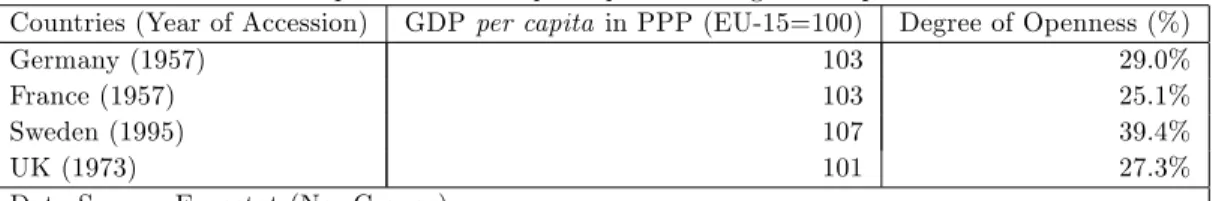
Sweden and the United Kingdom have repeatedly refuse to join the Euro. These are developed economies, with GDP per capita comparable to, or even higher than Germany and France, values that are shown in Table 1. By the time of the introduction of the Euro, in 1999, Sweden is more open than Germany
and France, and the UK had roughly the same degree of openness.3
Table 1- Comparison of GDP per capita and Degree of Openness in 1999
Countries (Year of Accession) GDP per capita in PPP (EU-15=100) Degree of Openness (%)
Germany (1957) 103 29.0%
France (1957) 103 25.1%
Sweden (1995) 107 39.4%
UK (1973) 101 27.3%
Data Source: Eurostat (NewCronos)
Business cycle synchronization is also an important decision factor to join the EMU. If business cycles are not synchronized, the impact of a common monetary policy is di¤erent for each country and may hurt the economy of the country. The ECB considers only the weighted average economic condition of the Euro-zone when setting monetary policy. Table 2 shows results for the cross-country correlations between the countries at study and the Eurozone. In Appendix A we have details on empirical data and methodological issues for these cal-culations. The superscript identi…es Eurozone variables. We can see that the cross-country correlations of output (Y ), consumption (c), and investment (I) are positive for all countries, behaving according to business cycles stylized facts. Labour (l) cross-country correlation for the UK is negative, although small. Sweden has the strongest degree of comovement with the Eurozone.
Table 2 - Cross-Country Correlations between the Countries and the EMU SWE UK
(Y; Y ) 0.77 0.66 (c; c ) 0.72 0.40 (I; I ) 0.71 0.48 (l; l ) 0.93 -0.05
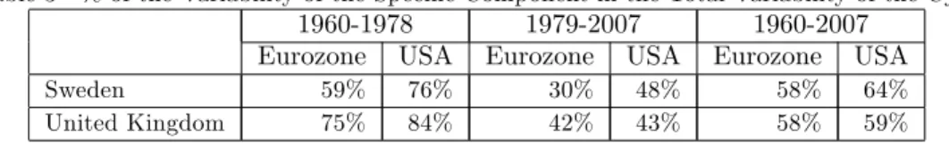
Also important is the proportion of the economic cycle of each country that is explained by an idiosyncratic component vis-a-vis a common component with the Eurozone. If the idiosyncratic component is very high that could be a prob-lem for EMU accession, because the lower the correlation between the economic cycle of a country and the Eurozone, the larger could be the welfare loss of
3Degree of Openness is calculated as [(exports+imports)/2]/GDP*100. The variables are
giving up monetary policy. For the sake of comparison we also present results regarding the common component with the USA. Results for the countries at study are presented in Table 3 and details on the estimations are in Appendix B.
Table 3 - % of the Variability of the Speci…c Component in the Total Variability of the Cycle 1960-1978 1979-2007 1960-2007
Eurozone USA Eurozone USA Eurozone USA
Sweden 59% 76% 30% 48% 58% 64%
United Kingdom 75% 84% 42% 43% 58% 59% Data availability allows us to divide the period between 1960 until 2007 in sub-periods. We choose to split the data in the year 1979 because it is the starting year of the European Monetary System. The weight of the speci…c component has been declining over time, although it is still high. The speci…c component of business cycle of the UK is more or less the same regardless whether we use the Eurozone or the USA, re‡ecting the strong relation between the UK and the USA, despite the accession to the European Union. Stock and Watson (2005) show that UK business cycle is less synchronized with the European business cycle and more with the North-American cycle, between 1984-2002. They also concluded that the percentage of the business cycle that it is explained by country speci…c factors is increasing, contrary to common factors, that are decreasing, contrary to what our results show. This is also one of the …ve economic tests that the British Government analyses from time to time in order to evaluate the bene…ts and costs of joining the EMU. Peersman (2007) using a two country structural vector autoregression (SVAR) also found a higher degree of business cycle synchronization with the US. Symmetric shocks with the Eurozone are important to explain UK output ‡uctuations, despite a strong presence of asymmetric shocks.
3
Model
We developed a dynamic equilibrium model in the tradition of Chari et al.(2002a), but modi…ed to take into account an interest rate rule similar to that suggested
by Taylor (1993) which also allows for forward looking behaviour. This setting permits us to construct a detailed quantitative analysis for the behaviour of the main macroeconomic variables and, more importantly, to quantify the wel-fare cost associated with the various policy choices. We provide a framework to evaluate the economic costs of joining the EMU, namely, to investigate the economic implications of the loss of the monetary policy ‡exibility associated with EMU and to assess the e¤ects of monetary policy in terms of welfare.
There are two countries in the model with a very large number of identi-cal consumers which will live forever, competitive …nal goods producers, and monopolistically competitive intermediate goods producers. This last group of agents sells their products to the …nal goods producers; the latter type of goods is non-traded. Trade between economies is in intermediate goods, produced by monopolists who can charge di¤erent prices in two countries. Intermediate goods prices are set on local market currency, each producer having the right to sell his goods in the two countries. Once prices are set, each intermediate goods producer must satisfy his demand.
The following goods exist in the economy in each period: labour, capital, real money balances, and a continuum of intermediate goods indexed by i 2 [0; 1] produced in the home country (identi…ed by a superscript H), and a continuum of intermediate goods indexed by i 2 [0; 1] produced in the foreign country (identi…ed by a superscript F ), which will be regarded as the EMU.
3.1
Consumers
In each period t = 0; 1; :::; consumers choose their allocations, facing the follow-ing budget constraints:
Ptct+Mt+Et+1QtBt+1 (1)
PtWtlt+Mt 1+Tt+Qt 1Bt+ t
where ct, lt and, Mtare respectively, consumption, labour, and money, Tt are
interme-diate goods producers, Pt is the price of the …nal good and Wtrepresents real
wages. The initial conditions M 1 and B0are given.
In this economy, there is perfect insurance between consumers in each coun-try. The asset structure is represented by having a set of government bonds designated Bt, which represents a vector of state contingent securities. Bt is
the foreign consumers’holdings of this bond. Qtis the vector of state contingent
prices for the bonds.
Consumers choose consumption, labour, real money balances, and bond holdings to maximize their utility:
E0 1 X t=0 tU (c t; lt; Mt=Pt) (2)
subject to the consumer budget constraints, where is the discount factor. The …rst order conditions for the consumer can be written as:
Ul t Uc t = Wt Utm Pt Utc Pt + Et+1 Uc t+1 Pt+1 = 0 Qt 1= Et 1 Uc t Uc t 1 Pt 1 Pt where Uc
t, Utl, and Utm are the derivatives of the variables of the utility
function. We can de…ne the nominal interest rate, rN, from the last …rst order condition: 1 1 + rN = Et+1 Uc t+1 Uc t Pt Pt+1
3.2
Final Goods Producers
In country H …nal goods are produced from intermediate goods through the following production function:
yt= 2 6 4a1 0 @ 1 Z 0 (yHi;t) di 1 A + a2 0 @ 1 Z 0 (yFi;t) di 1 A 3 7 5 1= (3)
where ytis the …nal good, yHi;tand yFi;tare intermediate goods produced in H and
F , respectively. Parameter determines the mark-up of price over marginal cost ( is the elasticity of substitution between goods produced in the same country, representing the market power of producers), along with , determine the elasticity of substitution between home and foreign goods. Parameters a1 and
a2, combined with and , determine the ratio of imports to output.
Final goods producers behave in a competitive way, in each period t, choosing inputs yH
i;tfor i 2 [0; 1] and yi;tF for i 2 [0; 1], and ytto maximize pro…ts subject to
(3). Prices are expressed in units of the domestic currency. Price of intermediate goods can at most depend on t 1, because producers set prices before period t. Factor demand functions are calculated by the resolution of the maximization problem and have the following expressions:
yi;tH=[a1Pt] 1 1 PH t 1 (1 )( 1) PH i;t 1 1 1 yt (4) yi;tF=[a2Pt] 1 1 PF t 1 (1 )( 1) PF i;t 1 1 1 yt (5)
where PHt 1is the average price of inputs and is equal to:
PHt 1= 0 @ 1 Z 0 Pi;t 1H 11 di 1 A 1
and PFt 1 is equal to:
PFt 1= 0 @ 1 Z 0 Pi;t 1F 11 di 1 A 1
since all producers behave competitively, their economic pro…t is zero, and the …nal good price is given by:
Pt= a 1 1 1 P H t 1 1 + a 1 1 2 P F t 1 1 1 (6)
which is independent of period t shocks.
3.3
Intermediate Goods Producers
Each intermediate good i, is produced according to a standard constant returns to scale production function:
yHi;t+yHi;t = F (ki;t 1; Atli;t) (7)
where ki;t 1 and At are respectively capital and technology used in the
pro-duction of the good, yH
i;t and yHi;t are the quantities of the intermediate good
produced in H, used in the production of the …nal good in country H and F , respectively. The law of motion for capital is given by:
ki;t= (1 ) ki;t 1+Ii;t
Ii;t
ki;t 1
ki;t 1 (8)
where Ii;t is investment, function (:) represents adjustment costs, and is the
depreciation rate. The initial capital stock ki; 1is given and is the same for all
producers in this group.
Intermediate producers behave as imperfect competitors, setting their prices in a staggered way. As usual this monopolistic setting ensures that output is determined by demand, at least in the short term when prices are …xed. Speci…cally, at the beginning of each period t, a fraction 1=N of producers in H choose a home currency price PH
i;t 1 for the home market and a price for
the foreign market. As these prices are set for N periods, for this group of intermediate goods producers: PH
i;t+ 1 = Pi;t 1H and Pi;t+H 1 = Pi;t 1H for
= 0; :::; N 1. Intermediate goods producers are indexed so that those with i 2 [0; 1=N] set prices in 0; N; 2N; and so on, while those with i 2 [1=N; 2=N] set prices in 1; N +1; 2N +1, and so on, for the N groups of intermediate producers. Consider, for example, producers in a group, namely i 2 [0; 1=N], who choose prices Pi;t 1H and Pi;t 1H , production factors li;t, ki;tand Ii;tto solve the following
problem: max E0 1 X t=0 Qt[Pi;t 1H yi;t 1H +
+etPi;t 1H yi;tH PtWtli;t PtIi;t] (9)
subject to (7), (8), and the constraints that their supplies to home and foreign markets, yH
i;t 1 and yi;t 1H , must equal the amount demanded by home and
foreign …nal goods producers, from equation (4) and analogue for F (equation (5)). Another constraint implies that prices are set for N periods. et is the
nominal exchange rate. Optimal prices for t = 0; N; 2N and so on, are:
Pi;t 1H = t+NP 1 =t E Q P vi; H t+NP 1 =t E Q H Pi;t 1H = t+NP1 =t E Q P vi; H t+NP 1 =t E Q e H
where vi;t is the real unit cost which is equal to the wage rate divided by the
marginal product of labour, Wt=Fi;tl Atand:
H t = [a1Pt] 1 1 PH t 1(1 )( 1)yt H t = [a2Pt] 1 1 PH t 1(1 )( 1)yt
in a symmetric steady-state real unit costs are equal across …rms, hence, in this steady state these formulas reduce to PiH= PiH = P v= , so that the law of one price holds for each good, and prices are set as a mark-up (1= ) over marginal costs P v.
3.4
Government
New money balances of the home currency are distributed to consumers in the home country in a lump-sum fashion by having transfers satisfy:
Ptgt+ Tt= Mt M(t 1) (10)
where gtis government consumption. This equation represents the home
gov-ernment budget constraint.
For our benchmark case we assume that the monetary policy rule for the Central Bank of country H follows a forward looking Taylor type interest rate rule. Several studies, for example Taylor (1993), have shown that the Taylor rule seems to replicate in an accurate way the monetary policy rule of Central Banks throughout the world. We follow the formulation of Clarida, Gali, and Gertler (2000), represented by:
rtN = rrNt 1+ (1 r)[ Et t+1+ oOt] + "r
N
t (11)
where rtN is the nominal interest rate in period t for the domestic economy,
( t+1= Pt+1
Pt 1) is the in‡ation rate between period t and t+1 for the domestic
economy, and Otis the real gross domestic product at t of the domestic economy. "rN
t are shocks with a normal distribution, zero average, r
N
standard deviation, and positive cross-country correlation. If r> 0 the rule exhibits some degree of inertia, as the Central Bank does not fully adjust to current changes in the economy.
Interest rates in country F , the Eurozone, are set according to the rule:
rNt = rrt 1N + (1 r)[$ Et t+1+ (1 $) Et t+1+
+$ oOt+ (1 $) oOt] + "r
N
t (12)
where $ is the weight of the home country’s GDP in the Eurozone (in simulation Common Monetary Policy), considering that the country is already a member. For the benchmark case, which we will explain in section 5, when the home country is outside the Eurozone (simulation Autonomous Monetary Policy), we set $ = 0. rN
t is the nominal interest rate in period t for the foreign
economy, ( t+1= Pt+1
the Eurozone, and Ot is the real gross domestic product at t of the Eurozone.
As usual, we allow for monetary policy shocks "rN
t with a normal distribution,
zero average, rN standard deviation, and no cross-country correlation. When
we use the Taylor rule of the ECB as the policy rule, the domestic economy has no monetary policy shock; we therefore imposed the following restriction on the nominal interest rate:
rNt = rNt (13)
3.5
Equilibrium Conditions
All maximization problems for country F are analogous to those of country H. An equilibrium requires several market-clearing conditions. The resource constraint in the home country is given by:
yt= ct+ gt+ 1
Z
0
Ii;tdi (14)
The labour market-clearing condition is:
lt=
Z
li;tdi (15)
similar conditions hold for the foreign country. The market-clearing condition for contingent bonds is:
Bt+ Bt = 0 (16)
The state of the economy when monopolists make their pricing decisions (previously of period t) must record the capital stocks for a representative mo-nopolist in each group in the two countries, the prices set by the other N 1 groups in both countries, and the period t 1 monetary shock but not period t monetary shock, and period t and t 1 technological and government consump-tion shocks. Period t 1 shocks help forecast the shocks in period t and current shocks are included in the state of the economy when the remaining decisions are taken. Consumers and …nal good producers know current and past realizations
of shocks. Monopolists know the past and current realizations of technolog-ical and government consumption shocks, but only know past realizations of monetary shocks.
We use the Blanchard and Kahn (1980) approach to solve the model. Several procedures are necessary: First, to make economies stationary we de‡ate all …rst order conditions for the nominal variables by the growth rate of prices mu; second, we derive the steady state equations and conditions for some stationary variables; third, we apply logs and linearize the …rst order conditions around the steady state, and …nally we solve the system of equations.4
4
Calibration and Data
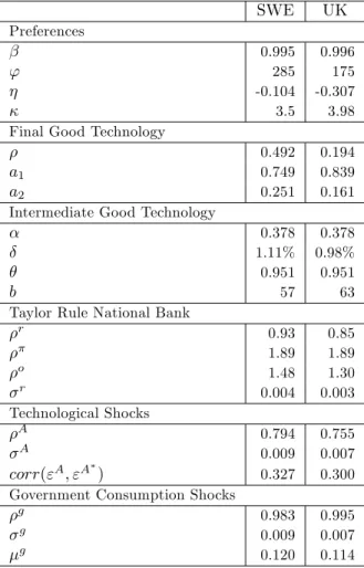
The calibration for the models is made in order to reproduce the long term prop-erties of each one of the economies at study. We use the calibration methodology suggested by Prescott (1986) and Cooley (1995). When needed, X12-ARIMA was used to remove seasonality and the Hodrick-Prescott …lter to detrend the data. Results for the parameters for each of the economies are reported in Table 4, at the end of this section.
4.1
Preferences
The functional form of the utility function is:
U c; l;M P = 2 4c(1 k ) (1 k ) + w(M P) 1 1 + ' (1 l)(1 ) 1 3 5 1 1 (17)
whose arguments are real consumption (c), labour (l), and a real money aggre-gate (M=P ). The discount factor is calculated using annual data, later turned into quarterly values, from AMECO, a European Commission annual database for = 1
(1+rLT), where rLT is the real long term interest rate for government
bond yields, which was de‡ated using the consumer price index, for the 1961-2007 period. The value for is 0.0001 for the two countries and k is the relative
4The growth rate of prices mu is calculated in order to respect the observed in‡ation rates
risk aversion coe¢ cient. In order to have a balanced growth we impose = . The weight on leisure, ', is calculated in order to make the time that families dedicate to work equal to a value that matches estimates from the Labour Force Survey of EUROSTAT, between 1983 and 2007 for the UK and between 1995 and 2007 for Sweden.
Parameters concerning money demand are estimated according to the …rst order condition for a nominal bond, which costs one euro at t and pays (1 + rN)
euros in t + 1: logMt Pt = log w 1 w+ log ct log rN t 1 + rN t (18)
we estimated regressions with quarterly data, where M 3 is used for M , the GDP de‡ator for P , private consumption at real prices for c, and the three month interest rate of the money market for rN.5 In the estimation we obtained the value for , the interest elasticity of real money demand, and the value for w is residual, which we set equal for the two countries. The period for the estimations is 1987:01-2007:04 and 1986:03-2007:04, respectively for Sweden and the UK.
4.2
Technology
4.2.1 Final Goods Producers
The elasticity of substitution between home and foreign goods is de…ned as
1
(1 ). Some studies, like that of Whalley (1985), found this elasticity to be in a
range between 1 and 2, and was lower for Japan and Europe than for the USA. We found the value for this elasticity by calculating the following regression, based on the …rst order condition of the demand functions for the intermediate goods:
logIM
D = b0+b1log P D
P IM+b2log Y (19)
5The monetary aggregate M 1 is the most correct aggregate to use, but, since data for M 1,
and even for M 2, is not available in Sweden, we choose to run this estimation with M 3 for both countries, for comparison reasons.
where IM , D, and Y are respectively imports, national production subtracted from exports, and national income, all at constant prices, P IM is the imports de‡ator, P D is the de‡ator for D. We use annual National Accounts data for 1970-2007 and 1980-2007, respectively for Sweden and the UK.
For the a1and a2parameters, representing respectively the weights of
domes-tic and imported goods, we used annual bilateral trade data from the CHELEM data base for 1990-2006. Shares for each country are calculated assuming that there are only two countries in the world, each one of the two countries and the Eurozone. yhand yf represent the share of imports from the Eurozone as a
per-centage of GDP and the share of national production as a perper-centage of GDP, respectively. To calculate a1 and a2 in their steady state values, the following
relation is used: yh=yf = [a1=a2]
1 1 .
4.2.2 Intermediate Goods Producers
The production function for intermediate producers is a Cobb-Douglas with constant returns to scale:
F (k; Al) = k (Al)1 (20)
We calculated the share of capital, , using OECD statistics for the capital income share of the private sector.
For the mark-up parameter we used data between 1993 and 2004 and 1970 and 2005, respectively for Sweden and the UK, taken from the NewCronos data base. In order to calculate the value for the markup parameter, we need to de…ne several variables. First, we de…ne the markup of price to marginal cost as PH=P
v = 1= . Then we need to de…ne pro…t as = y vy, where v is the
unit cost. In steady state v = , so =y = 1 . To obtain a estimate of =y we follow Domowitz et al. (1986) and de…ne the price-cost margin as (value added payroll)=(value added + cost of materials). In the steady state of the model the numerator of the former equation equals + (r + ) k. We calculate the denominator as Jorgenson et al. (1987), assuming that the value for the
cost of materials is similar to the value added. We then calculate the steady state values for (r + ) and k=y. The previous calculations imply the value for =y. Using the last value, we …nd the markup, which implies the value for .
We choose the number of periods that prices stay …xed for each group of producers, based on Gali et al. (2001) estimates that the number of quarters that price stay …xed in Europe to be about six, so we use this value for the two countries.
Capital Accumulation The depreciation rate for capital, , was calculated implicitly by the following formula:
Kt= (1 ) Kt 1+ It (21)
The data series for the capital stock and gross …xed capital formation (GFCF) was taken from AMECO, for the period between 1960-2007.
Adjustment Costs The adjustment cost function has the following expres-sion: I k = b I k 2 =2 (22)
the function is convex and satis…es the conditions f ( ) = 0 and f 0( ) = 0, implying that total and marginal costs of adjustment in steady-state are zero. b is the adjustment costs parameter.
4.3
Shocks
4.3.1 Technological Shocks
The technological shocks or supply shocks, Atand At, respectively for the home
and the foreign economy, are common to all intermediate goods producers of each country, following a stochastic process:
log At+1= Alog At+"At+1 (23)
log At+1= Alog At+"At+1 (24)
where technological innovations "A and "A have a normal distribution, with
zero mean, and A standard deviation, and are cross-country correlated but
are not correlated with the monetary and government consumption shocks. We estimate a V AR[1] for each one of the two economies and the Eurozone for the period between 1995:01-2007:04. Solow residuals were estimated using labour data only, because quarterly capital stock data is not available for these coun-tries, as in Backus et al. (1994).
4.3.2 Government Consumption Shocks
Government consumption shocks or demand shocks are modelled as stochastic processes, with the following expressions:
log gt+1= (1 g) g+ glog gt+ "gt+1 (25)
and
log gt+1= (1 g) g+ glog gt + "gt+1 (26)
where government shocks "g and "g have a normal distribution, with gmean, g standard deviation. These shocks are not correlated with monetary shocks,
with technological shocks, or with the foreign government consumption shocks. We use quarterly data from the EUROSTAT National Accounts for the period between 1980:01-2007:04 and 1955:01-2007:04, respectively for Sweden and the UK, to estimate the parameters.
4.3.3 Monetary Policy Shocks
In this model the National Central Bank follows a Taylor Rule, represented by equation (11). For the two countries the rule of the National Central Bank ex-hibits a positive correlation of 0.1 with the foreign monetary shock. We assume
this, since these countries, although outside the Eurozone, are hit by common shocks, so monetary policy rules usually can have some level of correlation.
The policy rule of the ECB is characterized by equation (12). For this insti-tution the parameters for r, , and O are 0.85, 1.48, and 0.60, respectively,
which were taken from Hayo and Ho¤man (2006). The volatilities of this rule di¤er between simulations for each country; these are 0.425% and 0.177% for Sweden and the United Kingdom, respectively. In the same order, their eco-nomic weight, $, is 4% and 19.7%. Policy rules for the UK and Sweden were based on Adam et al. (2005) and Sturm and Wollmershaüser (2008), respec-tively.
We kept a …xed exchange rate in the simulation where the ECB is in charge of monetary policy, calibrating it with the most recent values for the nominal exchange rate, for each country.
The variances of the three shocks were calculated in order to reproduce the volatility of output close to empirical data.
4.4
Summary
Table4 - Calibration Values for the Two Countries SWE UK Preferences 0.995 0.996 ' 285 175 -0.104 -0.307 3.5 3.98 Final Good Technology
0.492 0.194
a1 0.749 0.839
a2 0.251 0.161
Intermediate Good Technology
0.378 0.378 1.11% 0.98% 0.951 0.951
b 57 63
Taylor Rule National Bank
r 0.93 0.85 1.89 1.89 o 1.48 1.30 r 0.004 0.003 Technological Shocks A 0.794 0.755 A 0.009 0.007 corr("A; "A ) 0.327 0.300
Government Consumption Shocks
g 0.983 0.995
g 0.009 0.007
g 0.120 0.114
In Sweden the trade share with the EMU is bigger and the elasticity of substitution between domestic and imported goods is higher. In the UK people spend most time working than in Sweden. The Taylor Rule for the UK is less smoother than the Taylor Rule for Sweden in simulations Autonomous Monetary Policy. These di¤erences are going to in‡uence the value of the results and play an important role in the decision process to join (or not) the EMU.
5
Results
5.1
Methodology
The main purpose of this work is to formally analyze the consequences of di¤er-ent rules for monetary policy, in terms of consumer welfare in the two economies. We therefore ask how much consumption consumers are willing to give (or
re-ceive) in order to remain indi¤erent between the Common Monetary Policy and the Autonomous Monetary Policy regimes. This corresponds to calculating the compensating variation associated to the full elimination of the Autonomous Monetary Policy regime. The welfare analysis follows the Lucas (1987) method. A simulation of 1000 periods was made in both regimes.6 In the Common Monetary Policy regime technological and government consumption shocks take place both in the domestic and foreign economy, whereas monetary shocks only occur in the foreign economy, representing the Eurozone. In the Autonomous Monetary Policy regime, both economies su¤ered all three shocks. Based on the simulated time series we calculate the average value of the utility function for both regimes. Given the average values, we calculated the compensating variation in terms of consumption in the following way:
U0( c0; l0; M=P0) = U1(c1; l1; M=P1)
where U0uses the values for c; l, and M=P of the Common Monetary Policy
regime and U1uses the values of the Autonomous Monetary Policy regime. The
value of represents the gains (or losses) of welfare in terms of consumption percentage.
The main purpose of this section is to analyze the behaviour of these economies in the presence of shocks, but we also verify if the model can replicate some of the main features of business cycle stylized facts. We …rst analyze the results for business cycles statistics of the simulated economies in the two monetary regimes. Tables A1 to A2 in Appendix A present the results of the statistics for simulations Common Monetary Policy and Autonomous Monetary Policy, for the domestic economy of the two countries.
The values of the statistics for the simulations support some of the stylized facts found in the literature and in the section of empirical evidence above, for instance, output is more volatile than net exports, but less volatile than
6Since we use a long period of time, 1000 periods, this is equivalent to simulate the economy
over a period of time and computing welfare as the sum of discounted period utilities, and then repeating it many times and taking the average of the welfare in each simulation.
investment. Autocorrelations are usually persistent as in the data.
In simulation Common Monetary Policy there are not monetary policy shocks in the domestic economy, since monetary policy is established by the European Central Bank, so volatility is lower in this simulation.
Comparisons of the behaviour of autocorrelations di¤er from country to country, and depend of the magnitude of the shocks and the comovements be-tween them, but persistence is on average higher in simulation Autonomous Monetary Policy. This is a logical result, since monetary policy is oriented towards the domestic economy, hence monetary policy stabilizes more the do-mestic economy, making variables more persistent.
Analyzing the cross-country correlations we …nd that simulation Common Monetary Policy has on average the higher cross-country correlations. This hap-pens because of the imposition of equation (13), so especially for consumption and investment, cross-country correlations are very high.
5.2
Welfare Calculations
The results based on the methodology described in the previous sub-section are presented in Table 5. Consumers are willing to give up consumption in order to live in an economy where the monetary policy is established by the National Central Bank in the two countries.
Table 5 - Welfare R esults for the T wo Econom ies - Benchm ark Simulations
c l M=P U
Sweden
Common Monetary Policy 0.213 0.207 0.489 206.39 -0.54% Autonomous Monetary Policy 0.213 0.207 0.488 206.60
UK
Common Monetary Policy 0.306 0.214 0.150 125.83 -0.47% Autonomous Monetary Policy 0.306 0.213 0.150 125.97
The nominal interest rate in the Autonomous Monetary Policy regime is on average higher than in simulation Common Monetary Policy, in accordance to what happens in these economies. These economies have a more aggressive in‡ation parameter in the Taylor Rule for the National Central Bank. As a result, when prices increase, the interest rate response is higher, bringing about
a higher drop in average consumption. Therefore, on average labour has to rise by less in order to satisfy the increase in consumption and also to satisfy output demand. The behaviour of labour explains why consumers prefer the Autonomous Monetary Policy regime. Labour in this simulation is on average lower; as a result there is more leisure and consumers are better o¤.
Nominal exchange rate stability can be one of the bene…ts of joining the EMU, since in simulation Common Monetary Policy both volatilities of the price ratio between countries and the real exchange rate are lower than in simulation Autonomous Monetary Policy. But as we can see, for these countries, the costs of relinquishing monetary policy are higher, even though exchange rate volatility is higher.
Results are also in agreement with some of the empirical evidence of Section 2, since results are similar for Sweden and the UK, as they were in the referred section.
The main di¤erences between simulations within each country are the volatil-ity of the monetary policy shocks, the parameters of the Taylor rules, and the di¤erence between who runs the monetary policy (i.e., Taylor Rule, with or without economic weights). The di¤erent welfare results for each country are explained obviously by di¤erent parameters, but most importantly by di¤er-ences regarding the magnitude of technological, government consumption, and monetary policy shocks. In the next section we are going to analyze and discuss some of these parameters.
6
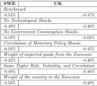
Robustness
In this section we analyze the robustness of the model in terms of the benchmark welfare value ( ) for the two countries.7 Results are presented in Table 6 below
and seem to be, on average, quite robust, reenforcing the decision of these countries not to join the EMU.
7We increase the correlations of monetary policy shocks in the Autonomous Monetary
Policy simulation to 0.5. We also increase the weight of imported goods from the Eurozone, as well as the weight of the country in the Eurozone (in simulation Common Monetary Policy ) to 25% more of their initial value.
Table 6 - R esults for Sensitivity A nalysis SWE UK Benchmark -0.54% -0.47% No Technological Shocks -0.49% -0.46%
No Government Consumption Shocks
-0.19% -0.02%
Correlation of Monetary Policy Shocks
-0.52% -0.45%
Weight of imported goods from the Eurozone
-0.42% -0.40%
Same Taylor Rule, Volatility, and Correlation
-0.49% -0.46%
Weight of the country in the Eurozone
-0.53% -0.40%
Generally we …nd that changes in the values of the weight of imported goods from the Eurozone and of the government consumption shocks seem to have the biggest impact in the change of the welfare value.
Technology shocks have a small impact on the welfare results, since the per-sistence of these shocks for these countries is lower than government spending shocks, but still the cost of entering EMU decreases with the disappearing of these costs. Although these shocks are positively cross-county correlated, much of its persistence has its e¤ects on the domestic economy, although much less than the government consumption shocks. Hence, when the shocks is eliminated so is the need to stabilize it. Since the output parameter of the Taylor rule of each the central banks of Sweden and the UK are higher they perform better at stabilizing these type of shocks The e¤ect of these shocks depends on the substitution and income e¤ects. In this model, and given the choices of para-meters for these countries, the substitution e¤ect prevails, so whenever there is a positive technological shock labour increases, and so does consumption.
Consumers are more indi¤erent between the two regimes, when demand shocks are removed. Volatility in both simulations are reduced and the need to stabilize idiosyncratic domestic spending shocks disappears, making consumers more willing to join the EMU. Results are stronger for the UK since the persis-tence of this shock is higher in this country.
Changes in the correlation of the monetary policy shocks also seem impor-tant, and make consumers in Sweden and in the UK more indi¤erent to the choice of regime. This is intuitive since increasing the correlation of mone-tary policy shocks in simulation Autonomous Monemone-tary Policy makes domestic and foreign nominal interest rates react in a similar way. As two policies be-come more alike, consumers bebe-come more indi¤erent between the two monetary regimes.
Also, we …nd that increases in the trade volume with the Eurozone decreases the costs of adopting a common monetary policy. This …nding is consistent with the theory of the endogeneity of optimum currency areas (Frankel and Rose, 1998). Higher trade shares increase the exposure of the country to foreign shocks and hence decrease the possibility of experiencing idiosyncratic shocks.
We conduct an experiment where we change the Taylor rule of the National Central Bank to be equal to the Taylor rule of the ECB, as well as its volatility and the cross-country correlation of the monetary policy shock, i.e., simulations become more alike. Sweden and the UK present lower costs of joining the EMU and relinquishing their monetary policy, but since these countries do not make the entire Eurozone alone, the cost still exists. The Taylor rule of the ECB is less volatile and also, for the case of Sweden, less smoother, being more aggressive and quicker in the stabilization process.
In order to assess the importance of the weight of the country in the monetary policy rule of the ECB we increase the weight of these countries in the Eurozone. Results are very intuitive, since now the countries have a smaller cost in joining the EMU. If the economic dimension of the country increases relative to the rest of the Eurozone, its in‡uence in the weighted average of the economic conditions of the EMU is also going to increase, and hence monetary policy is more suitable for its economic conditions. This is especially relevant in the case of the UK, where costs decrease signi…cantly.
7
Conclusions
The use of this model for these two countries illustrates in an explicit way the main result of this work: consumers are willing to give up part of their consump-tion in order to stay in an economy where the monetary policy is conducted on a national level. We must emphasize the fact that these results were obtained in the context of a complete markets model, making them even more important, because, even in a situation where consumers share the risk across countries, they are on average not willing to join the Eurozone.
Detailed analysis of the results shows that the loss of monetary policy ‡exi-bility is more or less costly depending on several factors. The decision of entering is more costly when government consumption shocks are stronger and when the trade share with the Eurozone is smaller, emphasizing the importance of the idiosyncratic features for these countries.
Besides discussing the costs of belonging to a Monetary Union, optimum currency area theory also discusses the bene…ts. It seems proper in this work to compare the results of the loss of independence of monetary policy with some of the bene…ts. One of the most important bene…ts of joining the EMU is the elimination of transaction costs. For UK there are several studies that try to assess the bene…t of loosing the exchange rate vis-a-vis the other EMU members. The European Commission (EC) in 1990 estimate this value to be 0.1% of GDP for the UK and 0.4% of GDP for the average of the European Union. In 1996, a study by IFO for the EC, claims that the last value had increased to 1% of GDP. Calmfors et al. (1997) found a 0.3% of GDP bene…t for Sweden. In countries which have a highly developed …nancial system, the gains from eliminating transaction costs are lower, since they have more …nancial products to defend themselves from exchange rate risk.
Converting our benchmark results to percentage of GDP, we …nd that in the two countries at study, consumers are willing to give up about 0.3% of their consumption in percentage of GDP to live in an economy with an autonomous Central Bank. Of course that the calculation of some bene…ts and costs are
excluded, but the values found in this work for the costs of the loss of monetary policy ‡exibility, are close to the bene…ts associated with the disappearance of transaction costs.
References
Adam, C., Cobham, D., Girardin, E., 2005. Monetary Frameworks and Institutional Constraints: UK Monetary Policy Reaction Functions, 1985-2003. Oxford Bulletin of Economics and Statistics 67, 497-516.
Backus, D. K., Kehoe, P. J., Kydland, F. E. (1994), “Dynamics of the Trade Balance and the Terms of Trade: The J-Curve?”, American Economic Review 84 (1), March, 84-103.
Beggs, D. et al., 2003. The Consequences of Saying No - An Independent Re-port into the Economic Consequences of the UK Saying No to the Euro. ReRe-port for the Commission, May.
Blanchard, O., Kahn, C., 1980. The Solution of Linear Di¤erence Models under Rational Expectations. Econometrica 48 (5), July, 1305 - 1311.
Brigden, A., Nolan, C., 2002. Monetary Stabilization Policy in a Monetary Union: Some Simple Analytics. Scottish Journal of Political Economy 49 (2), 196-215.
Calmfors L. et al., 1997. EMU - a Swedish Perspective. Kluwer Academic Publishers.
Carré, M., Collard, F., 2003. Monetary Union: a Welfare Based Approach. European Economic Review 47, 521-552.
Ca’Zorzi, M., Santis, R. A. de, Zampolli, F. , 2005. Welfare Implications of Joining a Common Currency. European Central Bank, Working Paper Series 445, February.
Chari, V.V., Kehoe, P. J., McGrattan, E. R., 2002a. Can Sticky Price Mod-els Generate Volatile and Persistent Real Exchange Rates? Review of Economic Studies 69 (3), July, 533-563.
Chari, V.V., Kehoe, P. J., McGrattan, E. R., 2002b. Technical Appen-dix: Can Sticky Price Models Generate Volatile and Persistent Real Exchange
Rates?. Federal Reserve Bank of Minneapolis, Research Department Sta¤ Re-port 277.
Clarida, R., Gali, J., Gertler, M., 1999. The Science of Monetary Policy: A New Keynesian Perspective. Journal of Economic Literature XXXVII, Decem-ber, 1661-1707.
Clarida, R., Gali, J., Gertler, M., 2000. Monetary Policy Rules and Macro-economic Stability. The Quarterly Journal of Economics 115, 147–180.
Cooley, T. F. editor, 1995. Frontiers of Business Cycles Research. Princeton University Press.
Corsetti, G., 2008. A Modern Reconsideration of the Theory of Optimal Currency Area. European Economy Economic Papers 308, March, European Commission, Directorate-General for Economic and Financial A¤airs.
Domowitz, I., Hubbard, R. G., Petersen, B. C., 1986. Business Cycles and the Relationship between Concentration and Price Cost-Margins. Rand Journal of Economics 17, 1-18.
European Commission, 1990. One Market, One Money. European Economy 44, Directorate-General for Economic and Financial A¤airs.
European Commission, 1996. Economic Evaluation of the internal market. European Economy Reports and Studies, 4, Directorate-General for Economic and Financial A¤airs.
Frankel, J. A., Rose, A.K., 1998. The Endogeneity of the Optimum Currency Area Criteria. Economic Journal 108 (449), 1009-1025.
Gali, J., Gertler, M., Lopez-Salido, J. D., 2001. European In‡ation Dynam-ics. European Economic Review 45, 1237-1270.
Goodfriend, M., King, R. G., 1997. The New Neoclassical Synthesis and the Role of Monetary Policy. NBER Macroeconomics Annual, 231-283.
Gros, D., Hefeker, C., 2002. One Size Must Fit All, National Divergences in a Monetary Union. The German Economic Review 3 (3), August, 247-262.
Hayo, B., Ho¤man, B., 2006. Comparing Monetary Policy Reactions Func-tions: ECB versus Bundesbank. Empirical Economics 31 (3), 645-662.
Holtemöller, O., 2007. The E¤ects of Joining a Monetary Union on Output and In‡ation Variability in Accession Countries. Mimeo. April.
Jorgenson, D., Gollop, F., Fraumeni, B., 1987. Productivity and US Eco-nomic Growth. Cambridge, Massachusetts, MIT Press.
Kenen, P., 1969. The Theory of Optimum Currency Areas: An Eclectic View. In: Mundell, R. and Swoboda, A. K. (Eds.), Monetary Problems of the International Economy, Chicago, University of Chicago Press, 41-60.
Lane, P., 2001. The New Open Economy Macroeconomics: A Survey. Jour-nal of InternatioJour-nal Economics 54 (2), August, 235-266.
Lucas Jr., R., 1987. Models of Business Cycles. Yrjö Jahnsson Lecture Series, Basil Blackwell Publishers.
Mackinnon; R. I., 1963. Optimum Currency Areas. American Economic Review 53, 717-725.
McAvinchey, I., McCausland, W.D., 2007. The Euro, Income Disparity and Monetary Union. Journal of Policy Modelling 29, 869-877.
Monacelli, T., 2000. Relinquishing Monetary Policy Independence. Boston College Working Papers in Economics 483.
Mundell, R., 1961. A Theory of Optimum Currency Areas. American Eco-nomic Review 51, March, 657-665.
Obstfeld, M., Rogo¤, K., 1995. Exchange Rate Dynamics Redux. Journal of Political Economy 103, 624-660.
Obstfeld, M., Rogo¤, K., 1998. Foundations of International Macroeco-nomics. MIT Press.
Peersman, G., 2007. The Relative Importance of Symmetric and Asym-metric Shocks: The Case of United Kingdom and Euro Area. Oesterreichische Nationalbank Working Paper No136, October.
Pesaran, M. H., Smith, L. V., Smith, R. P., 2007. What if the UK or Sweden had Joined the Euro in 1999? An Empirical Evaluation Using a Global VAR. International Journal of Finance and Economics 12, 55-87.
Carnegie-Rochester Conference on Public Policy 24, 11-44.
Stock, J. H., Watson, M. W., 2005. Understanding Changes in International Business Cycle Dynamics. Journal of the European Economic Association 3 (5), September, 968-1006.
Sturm, J.E., Wollmershaüser, T., 2008. The Stress of Having a Single Mon-etary Policy in Europe. CESifo Working Paper No 2251, March.
Taylor, J., 1993. Discretion Versus Policy Rules in Practice. Carnegie-Rochester Conference Series on Public Policy 39, 195-214.
Whalley, J., 1985. Trade Liberalization Among Major World Trading Areas. Cambridge, Massachusetts, MIT Press.
Woodford, M., 2003. Interest and Prices - Foundations of a Theory of Mon-etary Policy. Princeton University Press.
8
Appendix A - Detailed Data Speci…cation for
Business Cycle Statistics and Results
Data was taken from the Quarterly National Accounts of NewCronos, an elec-tronic database from EUROSTAT. The variables used are output (y), private consumption (c), investment (I), net exports as a percentage of GDP (nx), all at constant prices, and labour (l). We used quarterly data for Sweden, the UK, and the Eurozone at 15 member countries for the period between 1995:01 and 2007:04. H-P …lter was used to remove the trend and X12-ARIMA was used to remove seasonality, whenever data was not seasonally adjusted. All variables are in logarithms except net exports as a percentage of GDP. The cross-country correlations are for each of the two countries and the Eurozone. Results are presented in the second column of Tables A1 and A2.
Table A1 - Statistics and Stylized Facts for Sweden Data Common Autonomous
Monetary Policy Monetary Policy Standard Deviations
Y 0.83 0.83 0.83
N X 0.68 0.27 0.44
Standard DeviationsRelative to GDP
c 1.03 0.52 0.62 I 5.84 2.74 3.23 l 1.34 2.38 2.44 Autocorrelations Y 0.86 0.45 0.42 c 0.79 0.54 0.59 I 0.61 0.53 0.57 l 0.92 0.62 0.61 N X 0.44 -0.50 -0.40 Cross-Country Correlations (Y; Y ) 0.77 0.79 0.19 (c; c ) 0.72 0.99 0.06 (I; I ) 0.71 0.99 -0.01 (l; l ) 0.93 0.53 0.12 (Y; N X) -0.07 0.14 0.05
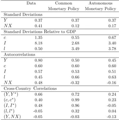
Table A2 - Statistics and Stylized Facts for The UK Data Common Autonomous
Monetary Policy Monetary Policy Standard Deviations
Y 0.37 0.37 0.37
N X 0.41 0.12 0.17
Standard DeviationsRelative to GDP
c 1.35 0.55 0.67 I 8.18 2.68 3.40 l 0.50 3.49 3.78 Autocorrelations Y 0.80 0.50 0.45 c 0.60 0.60 0.60 I 0.57 0.53 0.51 l 0.45 0.66 0.63 N X 0.48 -0.32 -0.16 Cross-Country Correlations (Y; Y ) 0.66 0.72 0.24 (c; c ) 0.40 0.99 0.23 (I; I ) 0.48 0.96 -0.05 (l; l ) -0.05 0.32 0.04 (Y; N X) -0.05 -0.03 -0.13
9
Appendix B - Some Further Business Cycle
Calculations
The data was taken from AMECO database, an online annual database of the European Commission. We estimated an OLS regression based on the following expression:
y_cict = 1y_cict 1+ 2y_cict 2+ 3y_cict+
4y_cict 1+ 5y_cict 2+ "t (27)
where y_cic is the cyclical component of real GDP of the domestic economy and y_cic is the cyclical component of real GDP of the foreign economy. "tcan be
regarded as the idiosyncratic component of the domestic economy ‡uctuations, i.e., the part of the domestic economy cycle that is not explained by the Eurozone business cycle (or alternatively the USA) nor by the past behaviour of the country cycle. The variables were detrended using H-P …lter with a value of 100. For each country we try several estimations in order to achieve the best possible …t. This means that whenever variables were not statistical signi…cant, they were removed.
Our purpose with these calculations was to assess the proportion of the business cycle explained by idiosyncratic shocks in each of the two countries. This proportion is calculated in the following way: "t
y_ cict, where "t is the
standard deviation of the idiosyncratic component of the cycle and y_ cict is
the total standard deviation of the cycle in the domestic economy. So, the bigger the value of this ratio, the bigger the proportion of the business cycle is due to speci…c country shocks. Our aim was also to compare the importance of the Eurozone and the USA in explaining the economic cycle of these countries, which is why we made two estimations for each country: one where the foreign economy is the Eurozone, and another where the foreign economy is the USA.