University of Algarve
Validation of a Method for the Analysis of Volatile
Organic Compounds in Water
Amresh Prasad Karmacharya
Erasmus Mundus Master in Quality in Analytical Laboratories
University of Algarve
Validation of a Method for the Analysis of Volatile
Organic Compounds in Water
Amresh Prasad Karmacharya
Erasmus Mundus Master in Quality in Analytical Laboratories
Thesis supervised by: Dr. Vitor Vale Cardoso Dr. Isabel Cavaco
i
Acknowledgement
This thesis research which involves method validation of VOCs with the use of SPME-GC-MS has been an excellent learning experience and an academic achievement for me. This has been possible with the guidance and assistance of several individuals and institutions and I am grateful to all of them.
First and foremost, I would like to express my sincere gratitude to my Supervisor Dr. Vitor Vale Cardoso for his expert guidance and constant support throughout my stay at the Central Laboratory of EPAL. He made sure that all the facilities needed for the research were readily available and manuscript corrected on time. He had answers for every question that I had.
Then, I would like to extend my sincere thanks to my co-supervisor Professor Dr. Isabel Cavaco for her moral support and for coordinating with EPAL. Actually, she has been supportive to me right from the beginning of the EMQAL program 2013-15.
I am also grateful to Antonio Pato who assisted me on the operational level in instrument operation, analytical procedure and trouble shooting. He was always available when I needed his assistance in the laboratory.
I would also like to thank Dr. Alexandre Rodrigues, Dr. Ana Penetra, Dr. Christina Correia, Dr. Ana Neto, Vania Constantino and Julia Valente of the Central Laboratory of EPAL for their suggestions and assistance. All the employees of the Organic Chemistry Lab made me feel comfortable throughout the study period.
I am also indebted to Eng. Maria Joao Benoliel, the Director, and Dr. Elisabete Ferreira, the Head of the Analytical Department, of the Central Laboratory of EPAL, Lisbon, for accepting my request and granting me access to the facilities of the laboratory for my research work.
Last, but not the least, I would like to thank, from the bottom of my heart, to the EMQAL Program of the European Union for granting me admission to the program and offering full scholarship without which I would not be able to attend and complete this program, visit Europe and experience new things.
Amresh Karmacharya
ii
Abstract
Many of the volatile organic compounds (VOCs) which can be harmful to humans have their origin in petroleum products. The VOCs have been found in water sources and leakage from storage tank and accidental spills have been regarded as the main causes of contamination from VOCs. The main objective of this study was to validate detection method of some 15 VOCs by solid-phase microextraction – gas chromatography – mass spectrometry. SPME-GC-MS has been a widely accepted method for analysis of VOCs.
The compounds analyzed in this study are; MTBE, 3-ethyltoluene, 4-ethyltoluene, 2-ethyltoluene, 1,2,4-trimethylbenzene, 4-isopropyltoluene, 1,3-diethylbenzene, Indane, 1,4-diethylbenzne, 1,3-dimethyl-5-ethylbenzene, 1,2-diethylbenzene, 1,4-dimethyl-2-ethylbenzenene, 1,3-dimethyl-4-ethylbenzene, dimethyl-4-ethylbenzene, 1,2-dimethyl-3-ethylbenzene and hexachlorobutadiene. After separation by the gas
chromatograph the compounds were detected in full scan mode and later further studies were carried out in selected ion monitoring (SIM) mode of mass spectrometer. Method validation parameters for the detection of these compounds included selectivity, linear working range, limit of detection (LOD), limit of quantification (LOQ) precision, accuracy and measurement uncertainty. Various statistical tools like regression analysis, residual analysis, Mandel’s test of linearity, RIKILT, and normalized area test were applied to derive and ascertain the results and arrive at a conclusion.
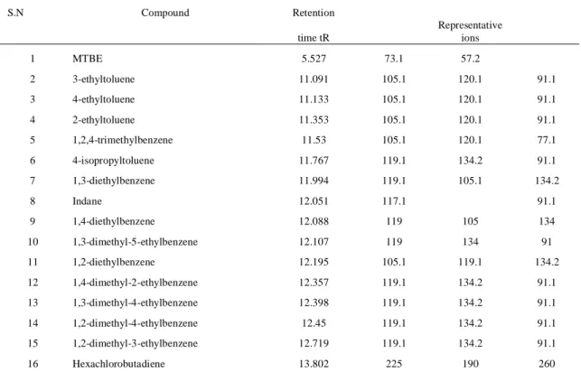
The retention time and representative mass fragments were identified for each compound. A linear curve (regression analysis) in the working range was also identified for each of these compounds after suitable dilution of the pure compounds. Working range was between less than 0.1 μg/L and 0.5 μg/L (the minimum and maximum calibration standards) for all the compounds except for MTBE and indane. Linearity was confirmed by residual analysis and Mandel’s test for linearity. Two of the compounds
1,4-diethylbenzene and 1,3-dimethyl-5-ethylbenzene coelute and appear as a single peak in the chromatogram and therefore, their quantity is expressed as the combined quantity of
iii the two. LODs are well above the baseline and LOQs are either equal to or lower than the lowest calibration standards. LOD and LOQ were also quantified from precision data. Precision was studied by determining repeatability and intermediate precision and was expressed as relative standard deviation (RSD %). Council Directive 98/83/EC has prescribed a limit value of 25% for precision. None of the values of repeatability and intermediate precision exceeded the limit of 25%. Accuracy was determined by recovery study of three types of spiked water matrices; tap water, river water and groundwater. Recovery was expressed by comparing the spiked results with the theoretical value (a value provided by the commercial supplier) of a compound in terms of percentage of recovery. Also 10 replicate analysis of the spiked sample gave its precision. Most of the recovery results have been found between 90 and 115%. All the recovery values meet the criterion of 25% recovery set by the Council Directive 98/83/EC.
ISO 17025 requires that the laboratories express the results accompanied by the estimated uncertainty. Expanded uncertainty of the method was determined for each compound by combining the component uncertainty of precision, calibration standards and regression interpolation and then multiplying the combined uncertainty by a coverage factor of two for a 95% confidence level. Uncertainty values ranged from 8.2% to 23%. It has been found that for the same compound the uncertainty values for the three different matrices are similar. VOCs targeted in this study can be used as possible indicators of petroleum product contamination of water sources. Each compound has its own retention time and mass spectra which can be used for its detection. Linearity of the working range has been confirmed by various statistical tests. LOD, LOQ and recovery results meet European regulation requirement and this indicates validity of the method and can be applied to detect the compounds in water. HS-SPME sampling is solvent free and less time consuming and therefore is preferable. There has been only limited research in method validation of many target VOCs. So this study contributes to methods of analysis used to detect the target VOCs in different water matrices.
Key words: VOCs, Petroleum, method validation, SPME, GC, calibration, LOD, LOQ, precision, accuracy.
iv
Table of Contents
ACKNOWLEDGEMENT... I ABSTRACT ... II TABLE OF CONTENTS ...IV LIST OF TABLES………...………..VII LIST OF FIGURES……..………...………VIII LIST OF ABBREVIATIONS……….IX LIST OF SYMBOLS……...………...………...X I. INTRODUCTION ... 1 1.1 Background ... 1
1.2 Introduction of target compounds ... 3
1.3 European Union policy related to water quality... 6
1.4 Solid-phase microextraction (SPME) ... 8
1.5 Gas chromatography and mass spectrometry ... 9
1.5.1 Gas chromatography ... 10
1.5.1.1 Gas chromatography instrumentation ... 17
1.5.1.1.1 Carrier gas ... 17 1.5.1.1.2 Injection mode ... 17 1.5.1.1.3 Chromatographic column ... 18 1.5.1.1.4 Stationary phase ... 19 1.5.1.1.5 Detectors ... 19 1.5.2 Mass spectrometry ... 20 1.5.2.1 Ionization source ... 21 1.5.2.2 Mass analyzer ... 22 1.5.2.3 Detector ... 22
1.6 SPME principle, apparatus and operation ... 23
1.7 Statistical tools for data analysis ... 25
1.7.1 Linearity and working range of calibration ... 25
1.7.2 Errors of regression equation ... 26
v
1.7.4 Working range ... 27
1.7.5 Tests for linearity Mandel’s test ... 27
1.7.6 RIKILT Test ... 28
1.7.7 Standardized area test... 29
1.7.8 Grubb’s test for outlier ... 30
1.8 Method validation ... 31
1.8.1 Selectivity ... 32
1.8.2 Linearity and working range ... 33
1.8.3 Limit of detection (LOD) ... 33
1.8.4 Limit of quantification (LOQ) ... 34
1.8.5 Precision ... 34
1.8.6 Accuracy ... 35
II. EXPERIMENTAL PROCEDURE... 37
2.1. Materials and reagents ... 37
2.2. Equipment and apparatus ... 37
2.3. Mass spectrometer ... 38
2.4. Analytical standards ... 38
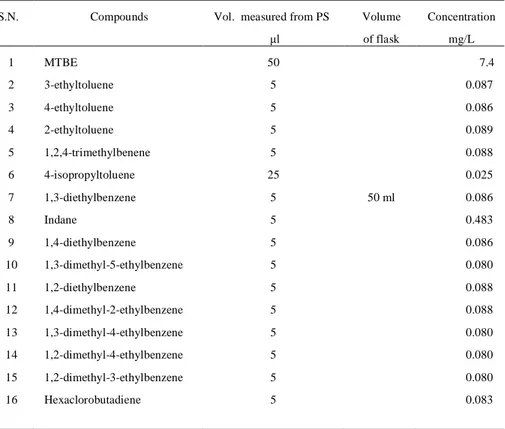
2.5. Preparation of intermediate and calibration solutions from the original standard solution, (standards supplied by the vendor) ... 38
2.5.1. Solution for optimization of the peaks ... 38
2.5.2. Linearity and working range ... 40
2.5.2.1. Preparation of primary (stock) solution from original standard solution ... 40
2.5.2.2. Preparation of Mix II from primary solutions ... 41
2.5.2.3. Preparation of Mix III from primary solution... 41
2.5.2.4. Preparation of Mix I from Mix II solution ... 42
2.5.3. Standard preparation for repeatability, intermediate precision and recovery studies ... 45
2.6. Solid-phase microextraction conditions ... 46
2.7. Gas chromatographic conditions ... 47
2.8. Mass spectrometric condition ... 47
III RESULTS AND DISCUSSION ... 48
3.1. Selectivity ... 48
3.2. Linearity and working range ... 60
3.2.1. Coefficient of determination r2 ... 62
vi
3.2.3. Mandel’s test ... 62
3.2.4. RIKILT test ... 62
3.2.5. Standardized (Normalized) area test ... 63
3.3. Precision ... 68
3.3.1. Repeatability ... 68
3.3.2. Intermediate precision ... 70
3.4. Limit of detection (LOD) ... 71
3.5. Limit of quantification (LOQ) ... 72
3.6. Accuracy... 73
3.6.1. Recovery in tap water ... 73
3.6.2. Recovery in river water ... 74
3.6.3. Recovery in groundwater ... 75
3.6.4. Comparison of recovery in the three types of water ... 76
3.7. Blank studies ... 77
3.8. Measurement uncertainty ... 78
IV CONCLUSION AND FUTURE PERSPECTIVE ... 81
REFERENCE ... 83
ANNEX
Annex I Residual analysis Annex II Mandel’s test Annex III RIKILT test
vii List of Tables
Table 1: A list of target compounds……….………..………...3
Table 2: A list of original standards used in the study………..……….39
Table 3: Physical properties of the compounds………..………....39
Table 4: Approximate minimum concentration required for detection..………...40
Table5: Preparation of primary solutions…………..……….……….…41
Table 6: Preparation of Mix II solution………..………..42
Table 7: Preparation of Mix III solution………..……….42
Table 8: Preparation of Mix I solution………..………....43
Table 9: Calibration standards for the 16 VOCs………..…………44
Table 10: Concentrations used for repeatability, intermediate precision and recovery……….….………...46
Table 11: GC temperature profile…….……….…………47
Table 12: Retention time and representative mass ions for each compound...……….49
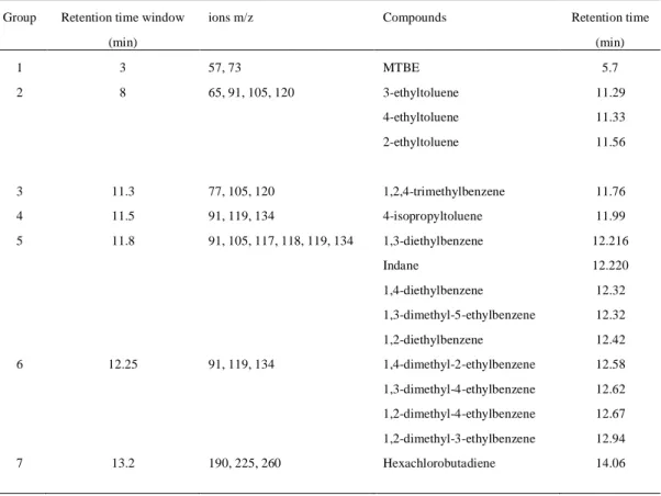
Table 13: Retention time window, the ion masses and the compounds………..……….58
Table 14: Calibration curve summary………...………….61
Table 15: Repeatability at low and high concentrations………...69
Table 16: Intermediate precision at low and high concentrations ………...70
Table 17: Comparison of LOD obtained from the three methods………...71
Table 18. Comparison of LOQ obtained from the three methods………...72
Table 19: Recovery of the compounds from the tap water………...74
Table 20: Recovery of the compounds from river water………...75
Table 21: Groundwater recovery at low and high concentrations……….76
Table 22: Comparison of recovery in the three types of water matrices………...77
viii List of Figures
Figure 1: Skeletal diagram of the target VOCs………...………....5
Figure 2: A chromatogram with different peaks……..……….10
Figure 3: Dead time and adjusted retention time……..………....12
Figure 4: A schematic diagram of a gas chromatograph………...18
Figure 5: A schematic diagram of a mass spectrometer………....21
Figure 6: Solid-phase microextraction assembly………. 24
Figure 7: Individual chromatogram and mass spectrum of the VOCs…..………57
Figure 8a: Peaks of the 15 target compounds in SIM mode……….……….59
Figure 8b: Peak of MTBE……….……….60
ix A list of abbreviations
CAR - Carboxen
EPAL - Empresa Portuguesa das Águas Livres GC-MS – Gas chromatography – mass spectrometry HS – Head space
MTBE – Methyl-tert-butyl-ether EU – European Union
SPME – Solid phase microextraction VOCs –Volatile organic compounds LLE – Liquid liquid extraction SPE – Solid phase extraction EI – Electron ionization LOD – Limit of detection LOQ – Limit of quantification DVB – Divinylbenzene
PDMS – Polydimethylsiloxane PS – Primary solution
RSD – Relative standard deviation FS – Full scan
SIM – Selected ion monitoring
ISO – International standards organization WHO – World Health Organization EM – Electron multiplier
PAT – Purge and tap
x A list of symbols
KD – Distribution constant tR – Retention time
tR’- Adjusted retention time tM – Hold-up time
k’ – Retention factor α – Selectivity factor
R – Chromatographic resolution N – Number of theoretical plates W1/2 – Peak width at half height H – Height of a plate
L – Length of column r – Correlation coefficient r2 – Coefficient of determination a – y-intercept
b – Slope of the calibration curve y – Instrument response
x – Concentration of unknown Sy/x – Residual standard deviation Sxo – Standard deviation of the method m/z – Mass to charge ratio
x̅ - mean of calibration standards y̅ - mean of instrument response yi – Experimental response ŷI – Predicted response yires – Regression residual
1
I. INTRODUCTION
1.1 Background
The topic of environmental pollution and adverse health impact it can cause, directly or indirectly, is no longer a topic of debate and, in a sense it has been an undesired part of our daily lives. Many categories of contaminants like heavy metals, pesticides, fertilizers, toxic organic compounds and greenhouse gases are released on land, into water bodies and atmosphere throughout the world. Huge quantities of fossil fuel (petrol or gasoline, diesel, kerosene, jet fuel, coal and natural gas) are consumed to meet the world’s ever increasing energy demand. Burning of fossil fuel inevitably emits greenhouse gases like carbon dioxide and methane, the biggest contributors to global warming. The other byproduct of fuel burning is the release of numerous health hazardous organic compounds. Toxic organic compounds are also released from other many synthetic commodities that people commonly use.
Many of the volatile organic compounds (VOCs) detected in soil and groundwater are toxic and mainly come from petroleum products like gasoline, diesel and jet fuel. VOCs like benzene, toluene, xylene, ethylbenzene (commonly called BTEX),
hexachlorobutadiene, methyl-tert-butyl-ether (MTBE) and many others originate from fuel burning. The second category of VOCs are chlorinated solvents used in various activities like dry cleaning, refrigeration, painting, pesticides, plastics and
pharmaceuticals.1-3 Examples of chlorinated solvents are trichloroethylene,
trichloroethane, carbon tetrachloride, methylene chloride, vinyl chloride among others.4
There are many more other VOCs that are emitted during combustion of petroleum. VOCs are hydrocarbons which are released from fossil fuel after incomplete combustion. The petroleum products are also used in plastics, fertilizers, paints, pesticides,
refrigerants, cleaning fluids, detergents, antifreeze and synthetic fibers.1 Gasoline mainly contains hydrocarbons, which have carbon atom C4-12, while diesel is composed of heavier fraction of C7-24. The hydrocarbons include alkanes, cycloalkanes, benzene, benzene derivatives and other monocyclic and polycyclic aromatic compounds.5 After
2 their release in the environment VOCs undergo transformation through physical,
chemical and biological processes. Most transformation in the environment especially in groundwater is caused by microorganisms.6
Subsurface spills of petroleum compounds may be the most frequently stated cause of groundwater contamination.7 Leaking underground and above ground tank and
accidental spills are major routes of soil and groundwater contamination and underground tanks being the most common cause.8 The leaking underground storage tanks containing petroleum products have contaminated groundwater and drinking water across the United States.9 After the spill or release, because of their volatility some VOCs evaporate away. The left over ones may be carried deep into the groundwater table by rain, water, or snow melt.10 Therefore, VOC concentrations found in groundwater may be many more times higher than that found in surface water11.
VOCs can react with sunlight and nitrogen oxides to produce ground level ozone which can cause lung and tissue damage [5]. Groundwater is a major source of drinking water, and groundwater contaminated with VOCs has been associated with human-health concern. Toxic effect of VOCs can vary which can range from being benign in its effect to being highly toxic. Benzene and formaldehyde are known human carcinogens. The health effect also depends upon nature and length of exposure. Long term exposure to VOCs can adversely affect liver, kidneys and central nervous system. Short term exposure to VOCs can cause eye and respiratory tract irritation, headaches and dizziness.12-15
The main objective of this study was to detect and identify mainly monocyclic aromatic VOCs by head space solid-phase microextraction followed by gas chromatography and mass spectrometry and validation of the analytical method. Most of these compounds have origin in petroleum products. Detection of these compounds in drinking water, surface water, wastewater or groundwater can be used as an indicator of petroleum contamination. A couple of the compounds have been regulated for drinking water or surface water use and have stipulated water quality standards within the European Union.
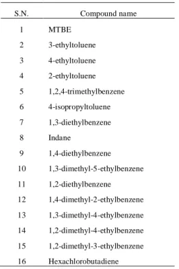
3 Following is a list of compounds (Table 1) that have been the focus of this study.
Table 1: A list of target compounds. S.N. Compound name 1 MTBE 2 3-ethyltoluene 3 4-ethyltoluene 4 2-ethyltoluene 5 1,2,4-trimethylbenzene 6 4-isopropyltoluene 7 1,3-diethylbenzene 8 Indane 9 1,4-diethylbenzene 10 1,3-dimethyl-5-ethylbenzene 11 1,2-diethylbenzene 12 1,4-dimethyl-2-ethylbenzene 13 1,3-dimethyl-4-ethylbenzene 14 1,2-dimethyl-4-ethylbenzene 15 1,2-dimethyl-3-ethylbenzene 16 Hexachlorobutadiene
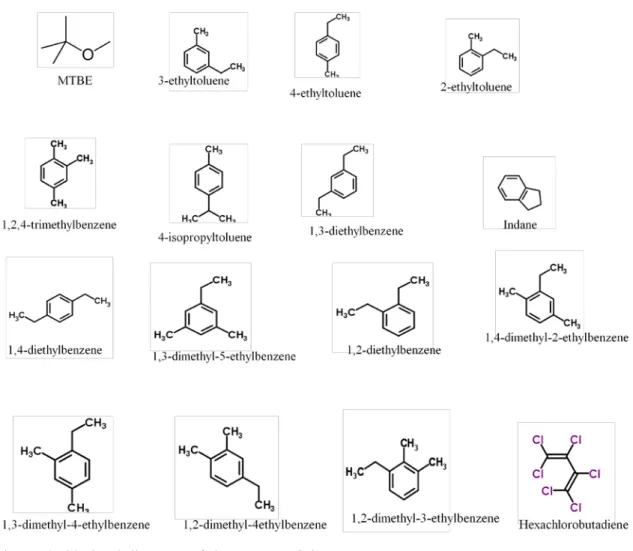
1.2 Introduction of target compounds
Hexachlorobutadiene
Hexachlorobutadiene is a clear colorless liquid. It is insoluble in water but soluble in ethanol (Figure 1). It is used in chlorine gas production and in manufacture of rubber compounds, lubricants and pesticide. In studies with oral introduction of hexabutadiene, kidney tumors were observed in rats. European Union has set hexachlorobutadiene maximum allowable concentration 0.6 μg/L in inland surface waters and WHO guideline value of drinking water is also 0.6 μg/L.16-18
Methyl-tert-butyl-ether (MTBE)
MTBE is a clear colorless liquid. It has a strong characteristic odour. There is a low risk of contamination in surface water due to its volatility. Spills and leakage of gasoline storage tanks can cause more serious groundwater contamination with MTBE where it is
4 more persistent. The major use of MTBE is as a gasoline additive to raise octane number. WHO mentioned a threshold value for odour of 15 μg/L. At high levels of exposure MTBE can cause cancer and non-cancer effects in laboratory animals.17,19
4-isopropyltoluene
4-isopropyltoluene is a flammable, colorless water insoluble liquid and has a
characteristic odour. It is used in the manufacture of paint and furniture. It can cause irritation of eyes and skin and the substance may be toxic to central nervous system and repeated or prolonged exposure can produce target organ damage. New York State human health fact sheet has established a threshold value for 4-isopropyltoluene as 5 μg/L in ambient water.20-23
Indane (Indan)
Indane is a clear colorless liquid. It is a type of hydrocarbon found in petroleum products. Indane is used as fuel for supersonic military aircraft. Environment Protection Agency of Ireland has categorized it as a hazardous substance.24-25
1,2,4-trimethylbenzene
1,2,4-trimethylbenzene is a clear colorless liquid with a distinctive odor. It is a byproduct of petroleum refining process. It is also used as a solvent in coatings, cleaners, pesticides and inks. Exposure to 1,2,4-trimethylbenzene can occur through inhalation, ingestion or contact with skin or eye. It can cause irritation of eyes, skin and respiratory system. It can adversely affect eyes, skin, respiratory system, central nervous system and blood. Based on human health criteria a concentration of 72 µg/L has been proposed for ambient water quality. 26-27
Diethylbenzene isomers
Diethylbenzene isomers include 1,2-diethylbenzene, 1,3-diethylbenzene and 1,4-diethylbenzene. They are clear colorless liquid which are insoluble in water.
Diethylbenzene isomers are components of petroleum products and are released to the environment as a byproduct of combustion in engines. The substance may enter body
5 through inhalation or ingestion. Short term exposure to diethylbenzene isomers can be irritating to eyes, skin and nervous system. The isomer 1,4-diethylbenzene has been suspected of inflicting adverse effect on kidney and liver.28-29
Figure 1: Skeletal diagram of the target VOCs
Ethyltoluene isomers
Ethyltoluene isomers are clear colorless liquid. They are flammable and volatile and water insoluble. Ethyltoluene is added to petrol to increase its performance. It can be released from petroleum refineries, petrol stations and in vehicle exhaust fumes. It can help to form ground level ozone. Ethyltoluene is an irritant of mucous membrane and upper respiratory tract. It may cause central nervous system effects. In laboratory animals it has been found to cause kidney, liver and reproductive system effects.30-31
6 Dimethylethylbenzene isomers
Isomers of dimethylethylbenzene that were included in this study are 1,3-dimethyl-5-ethylbenzene, 4-1,3-dimethyl-5-ethylbenzene, 1,3-dimethyl-4-1,3-dimethyl-5-ethylbenzene, 1,2-dimethyl-3-ethylbenzene and 1,4-dimethyl-2-ethylbenzene. These isomers also originate from petroleum products and therefore can be used as indicators or petroleum contamination of water sources. Information available on toxicity of these compounds are rather limited.
1.3 European Union policy related to water quality
Since 1975 a number of EU Directives and Regulations have been promulgated which have specified the quality of waters required for different uses. The legislation is aimed primarily at the safeguarding of human health by protecting water resources in general and for particularly human consumption.32 Following are some of the Directives that are directly related to water quality issues.
Surface Water Directive 75/440/EEC33
This Directive was promulgated in 1975. Its main objective was to address the concern of the quality of surface water that is intended to be abstracted for human consumption after treatment. Groundwater was not subject to this Directive. It has set the threshold values of the surface water quality. Phenols and PAH are the VOCs mentioned in the standard. This directive has been repealed by the Directive 2000/60/EC.
Bathing Water Directive 76/160/EEC34
This Directive was also promulgated in 1975. It addresses the protection of waters used for bathing but it does not include swimming pools. Member states are required to set the threshold values of bathing waters. Bathing Water Directive has laid down quality
requirement for all freshwater and sea waters defined as bathing waters. Among the VOCs, threshold for phenol was included.
7
Groundwater Directive 2006/118/EC35
This was promulgated in 2006 and addresses the issue of protection of groundwater. Member states have to establish threshold values for the parameters given in the Directive. Trichloroethylene and Tetrachloroethylene are the VOCs that the member states should monitor.
Drinking Water Directive 80/778/EEC36
This Directive was related to the quality of water intended for human consumption. For the parameters given the member states should fix the threshold less than or same as the values Maximum admissible concentration. The organic parameters covered were PAHs, PCBs and organochlorine, for example. This directive has been repealed by the Council Directive 98/83/EC.
Council Directive 98/83/EC37
The objective of the Directive is to protect human health from adverse effects of any contamination of water intended for human consumption. Human consumption includes drinking, cooking and other domestic purposes. Regular monitoring of water quality is required and analytical methods have been listed in Annex III. Commission Decision 2002/657/EC38 has given performance criteria and validation parameters for the
analytical methods for testing water quality. Council Directive 98/83/EC has laid down standards for many water quality parameters.
Following are the quality standards of VOCs.
Benzene 1.0 μg/L
Benzo(a)pyrene 0.01 μg/L
1,2-dichloroethane 3.0 μg/L
PAHs 0.10 μg/L
Tetrachloroethene and trichloroethene 10 μg/L
Trihalomethanes 100 μg/L
8 Similarly, Directive 2008/105/EC39 is on environmental quality standards in the field of water policy. It has given an extended list of standards of priority substances for surface waters. Among the VOCs it includes benzene, carbon tetrachloride, 1,2-dichloroethane, dichloromethane, DEHP, hexachlorobutadiene, naphthalene, pentachlorobenzene, pentachlorophenol, PAH, benzo(a)pyrene, tetrachloroethylene, trichloroethylene, trichlorobenzene and trichloromethane, for example.
1.4 Solid-phase microextraction (SPME)
Sample extraction is an important step of sample preparation meant for subsequent separation and detection of the compounds by gas chromatography or liquid
chromatography. Physico-chemical characteristics like molecular weight, boiling point and polarity of an organic compound can indicate the solubility of that compound in water. Based on some of the above mentioned characteristics different types of compounds may be extracted by different extraction techniques.40 In general organic compounds with smaller molecules are more volatile and less polar.
Several sample extraction techniques have been applied for analysis of organic
compounds in different matrices. Liquid-liquid extraction (LLE), solid phase extraction (SPE), purge and trap (PAT or dynamic head space), static head space, immersion solid- phase microextraction and head space solid phase microextraction (HS-SPME) are some of the most commonly used techniques for extraction of organic compounds from water. LLE 41-43 and SPE 44-46 are mostly used for polar and water soluble compounds. Direct SPME has been used for both polar compounds and VOCs.45-48 Present study has employed head space solid-phase microextraction (HS-SPME) as the sample extraction technique to extract VOCs from water.
In LLE and SPE solvent wastes are generated, multiple operation steps are needed and interfering compounds are more likely to be extracted.49 Many investigators have
considered SPME a viable technique for overcoming matrix effects in samples.49-51 It is a quick and handy method which integrates different steps of sample preparation like sampling, extraction, concentration and sample introduction in one single step. This saves
9 time, reduces cross-contamination and loss of analytes and does not generate solvent waste.52-54
In SPME analytes are extracted from the matrix by fused silica fiber coated with a polymeric stationary phase. SPME can be performed in two ways, immersion or direct sampling and head space sampling (HS-SPME). In direct sampling the silica fiber is immersed in the sample itself whereas in headspace sampling the fiber is exposed in the headspace of a sealed container.55 Headspace techniques are more suitable for extracting VOCs. Headspace techniques may be static, dynamic (purge and trap) or SPME. Many studies have found HS-SPME useful in detecting VOCs.48,54,56-57 although purge and trap is also considered a good extraction technique.58-60 Headspace techniques are generally coupled to gas chromatograph and HS-SPME coupled with GC-MS has been extensively used in the analysis of VOCs.43,49,61-64 Because SPME is so simple yet effective it has been accepted even by the official methods and standards: ASTMD6520, ASTMD6889, EPA Method 8272 and ISO 27108.65-68 Normally, direct SPME is coupled to liquid chromatography for detection of the compounds that are soluble in liquid phase, weakly volatile and thermally labile.69-71
1.5 Gas chromatography and mass spectrometry
Gas chromatography and mass spectrometry have been used for separation, identification and quantification of the volatile organic compounds for a long time. The technique is very efficient and widely practiced. A gas chromatograph separates the compounds according to the retention time and mass spectrometer detects the compounds eluted from GC and quantifies them. Because of ever increasing demand for analysis of a variety of harmful compounds its use has become more and more important and with time the technology has made a lot of advancement. GC-MS technique has been used for analytical purposes in a variety of materials like food and beverage products,
pharmaceutical products, and environmental media. Many studies have focused on the compounds released from petroleum products and other chemicals used in refrigeration, dry cleaning, painting, degreasing etc. Benzene, toluene, ethylbenzene and xylene (BTEX) and MTBE have been studied for many years by many investigators in drinking
10 water and natural waters.72-76 Similarly, analysis of compounds of biological origin have also been a common practice.77-80
1.5.1 Gas chromatography
Gas chromatography is a technique that is used to separate a mixture into its individual components and identify and quantify the unknown compounds. Like for other
chromatography, GC requires a mobile phase which is an inert gas (hydrogen, helium) and a stationary phase which makes the separation possible. The stationary phase is a solid or liquid coated on a solid support. Because, the different analytes interact
differently with the stationary phase they are carried out by the mobile phase in different rates. Some are carried sooner than the others. The individual compounds separated by the gas chromatograph are detected by a detector and translated into a chromatogram. The compounds are represented by peaks in the chromatogram. Each peak corresponds to one compound and each peak appears from the column after specific time period. In the chromatogram (Figure 2) detector response (y-axis) is plotted against the elution time or retention time (x-axis). The position of the peaks in the retention time axis serves to identify a compound and the area of the peak provides the quantity (concentration) of the compound in the mixture.
11 Theory of separation
When a sample is injected into a gas chromatograph the molecules of the compound interacts with the stationary phase as the analyte molecules are carried by the mobile phase. Selective partitioning of the analyte between the mobile phase and the stationary phase depends on the analyte molecule’s nature of interaction with the stationary phase. The compounds that interact strongly are retained longer in the stationary phase and are released late. Therefore their elution takes longer time. This time taken for a compound to get eluted from the column is called retention time. The most common interactions between the compounds and the stationary phase that play major role in giving relative retention times to different types of compounds are the non-covalent interactions, namely, dispersion, dipole and hydrogen bonding. The type of interaction depends on polarity of the compounds and the stationary phase. Polar compounds are retained for a longer time in a polar stationary phase and non-polar compound in a non-polar stationary phase.
Chromatographic parameters
Followings are a brief description of some of the important chromatographic parameters.
Distribution constant81
It was mentioned earlier that the separation of the different compounds are based on the selective partitioning of the compound between the mobile and the stationary phase. An analyte is in equilibrium between the two phases represented by the following equation.
KD
Amobile --- Astationary Distribution constant KD = Cs/Cm Amobile: Analyte quantity in mobile phase
Astationary: Analyte quantity in stationary phase Cs : concentration of analyte in the stationary phase Cm : concentration of analyte in the mobile phase
12 The equilibrium constant for this reaction is called distribution constant, or partition coefficient or partition ratio KD which is the ratio of the compound in the stationary phase and in the mobile phase. Higher KD values indicate that the compound is more adsorbed in stationary phase than it is in the mobile phase.
Retention time (tR)
The time taken for a compound to travel between the sample injection and detection by a detector after elution is called retention time. Therefore, it is the total time the compound spends in mobile and stationary phase. Usually each analyte in a sample will have a different retention time. Sometimes more than one compound interacts with the stationary phase in the same manner and they may have the same retention time. This results in a single peak that represents more than one compound. Such a condition is called
coelution. In this study also two of the 17 compounds studied coelute and have the same retention time. The separation of coeluted compounds may be achieved by using a stationary phase with a different polarity or by the signature mass fractions of the compounds given by the mass spectrometric detection.
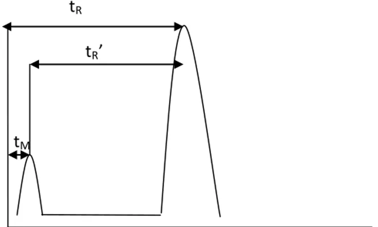
Dead time (hold-up time) tM and adjusted retention time tR’
Dead time is the time taken to travel for a compound in the absence of retention in the stationary phase. Adjusted retention time is the peak’s retention time minus the dead time.
tR tR’
tM
13 Retention factor k’ (capacity factor)
Retention factor is often used to describe migration rate of an analyte on a
chromatographic column. Mathematically, it is a ratio of the adjusted retention time and the hold-up time.
k’ = tR’/ tM = (tR – tM)/tM
When retention factor is much less than one, elution occurs rapidly, and when it is much larger elution time becomes much longer. It is a measure of the time the sample
component resides in the stationary phase relative to the time it resides in the mobile phase. Retention factor is defined as the quantity of solute in the stationary phase (s) divided by the quantity in the mobile phase. The quantity of solute in each phase is equal to its concentration (Cs or Cm) times the volume of the phase (Vs or Vm). Retention factor is a measure of solute velocity through a chromatographic column compared to the mobile phase.
k’ = (Cs . Vs)/(Cm . Vm)
Cs/Cm = KD, the Distribution constant
Chromatographic resolution (R)
Resolution is a measure which tells us how well two species have been separated. It takes the width of the chromatographic peaks into account. Separation and enough resolution is the goal of chromatography. Mathematically, resolution R between two compound A and B is given by;
R = 2(tRB – tRA)/(WA +WB)
tRB = retention time of the second peak tRA = retention time of the first peak WA = width of the first peak
14 An R value of 1.5 gives the separation at the baseline of the chromatogram. The
resolution for a given stationary phase can be improved by increasing column length which increases the number of theoretical plates. A high resolution chromatographic column separates peaks down to the baseline of the chromatogram.
Column selectivity
Selectivity of a column depends on relative migration rates of the compounds being separated. The relative migration rates of A and B is given by the ratio of the distribution constants of A and B. This is called selectivity factor α. Selectivity factor is a measure of the amount of peak separation.
α = KDB/KDA
The relationship between the selectivity factor and retention factor is given by;
α = k’B/k’A = (tRB – tM)/(tRA – tM)
When calculating the selectivity factor, species A elutes faster than species B. The selectivity factor is always greater than 1. If α = 1 then the peaks have same retention time and thus they coelute.
Column efficiency and band broadening
Band broadening is the increase in width of a peak and this happens because of increase in retention time due to more interaction of a compound with the stationary phase. All the peaks in a chromatogram do not have equal widths, some are narrower and others are wider. A chromatogram with narrower peaks can accommodate more numerous peaks with less overlapping, if any. In other words more compounds can be separated if the peaks are narrow. Column efficiency is the ability of a column to separate compounds from a mixture. Greater the column efficiency, the higher the number of compounds that can be separated. Band (peak) broadening causes the column to be less efficient.
Quantitatively, column efficiency may be expressed as the number of theoretical plates (N) and plate height (H) described by the theoretical plate model. A column with lower N
15 has more overlapping peaks and with higher N has thinner peaks. The plate model
supposes that the chromatographic column contains a larger of separate layers called theoretical plates. Improving the efficiency of a column would be to increase the number of plates and decrease the plate height. The theoretical plates are imaginary sections and the number of theoretical plates is related to retention time and width of the peak of a compound.
N = 5.45 (tR/W1/2) N = number of theoretical plates
tR = retention time
W1/2 = peak width at half height
N varies depending on compound as well as packing material. N also varies with the flow rate and the column length. Efficiency can also be measured by the height of a plate (H). The column efficiency increases as the plate height becomes smaller.
H = L/N H = height of a plate
N = total number of theoretical plates L = column length
Rate theory of chromatography
This theory takes into account time taken for the solute to equilibrate between the stationary and the mobile phase; the plate model does not take time into account. The resulting band shape of a peak is affected by rate of elution (flow rate of mobile phase). It is also affected by the different paths available to solute molecules as they travel between particles of stationary phase. If we consider the various mechanisms which contribute to band broadening, we arrive at the VanDeemter equation for plate height.
HETP (H) = A + B/u + Cu = A + B/u + (CS + CM)u u = average velocity of the mobile phase
A is Eddy diffusion: The mobile phase moves through the column which is packed with stationary phase. Solute molecules will take different paths through the stationary phase
16 at random. This will cause broadening of the solute band, because different paths are of different lengths.
B is Longitudinal diffusion: The concentration of an analyte is less at the edges of the band than at the center. Analyte diffuses out from the center to the edges. This causes band broadening. If the velocity of the mobile phase is high then the analyte spends less time on the column which decreases the effects of longitudinal diffusion.
C is Resistance to mass transfer: The analyte takes a certain amount of time to equilibrate between the stationary and mobile phases. If the velocity of the mobile phase is high, and the analyte has a strong affinity for the stationary phase then the analyte in the mobile phase will move ahead of the analyte in the stationary phase. The band of analyte is broadened. The higher the velocity of mobile phase, the worse the broadening becomes.
Peak capacity nc
It is the maximum number of peaks that can be fitted in a chromatogram or in other words the number of solutes that can be separated. Quantitatively, peak capacity nc is given by the following equation;
nc = 1+ (√(N))/4ln(Vmax/Vmin)
N = number of theoretical plates
Vmax = largest volume of the mobile phase in which we can elute and detect a solute Vmin = smallest volume of the mobile phase in which we can elute and detect a solute
Peak symmetry
It is assumed that solutes elute as a normal (Gaussian) peak. Peak tailing occurs when some sites on the stationary phase retain the solute more strongly than other sites. Peak fronting is most often the result of overloading the column with sample. Peak symmetry is determined by bisecting the peak through the apex. The width at 10% height is measured for each half. The width of the back half is divided by the width of the front
17 half. A perfectly symmetrical peak has a symmetry factor of 1.00 and larger deviations from 1.00 may be an indicator of peak tailing or peak fronting.
1.5.1.1 Gas chromatography instrumentation
It has already been mentioned that GC separates compounds by passing the vaporized mixture through a tube containing a material that non-covalently interacts with the solutes in the mixture. The type and degree of interaction is different for different compounds and therefore they are retained in the column for different periods of time. Gas
chromatograph is used to perform separation of the compounds. Gas chromatograph consists of a source of gas as mobile phase, an injection port, chromatographic column, a detector and the data display system.
1.5.1.1.1 Carrier gas
Carrier gas acts as the mobile phase which carries the samples through the instrument. The most common gas used is helium although sometimes hydrogen or nitrogen is also used. The carrier gas should be of high purity (99%). Gas purifiers may be used to
produce high purity gas. For the present study helium was used as the carrier gas. Helium is suitable for the stationary phase of the gas chromatograph used in this study.
1.5.1.1.2 Injection mode
Chromatographic process begins when a sample is introduced into the instrument at the injection port. The sample is injected with the help of a syringe manually or
automatically by using a robotic system. In the present study, an automatic sample injector was used. Injector port has a heated glass liner in which liquid sample is vaporized to be carried by the carrier gas or if sample is a vapor then it will not get condensed. The SPME fiber, used in this study desorbs its adsorbed solutes upon heating in the injector.
18 Figure 4: A Schematic diagram of a gas chromatograph
Injection can be split or splitless. Sample injection in gas chromatography depends on the nature of the sample. Sample volume should be kept to a minimum for best column efficiency. The concentrations of many samples can exceed the capacities of a column being used. Therefore, quantity of excess sample has to be reduced before it reaches the column. Split injector divides the total sample into two parts and allows only the smaller part to enter into the column. The large portion is vented away. However, when sample contains sufficiently lower concentrations (trace level) of an analyte, splitless injector is used. Splitless injector sends all the injected sample into the column. Most injectors can act both in split and splitless modes. The present study used splitless mode since analytes were injected at trace level.
1.5.1.1.3 Chromatographic column
Column is considered the heart of a gas chromatograph because the main activity of chromatography, the separation of the solute, takes place inside the column. Usually the
19 separation is temperature dependent and the desired temperature is maintained by placing the column in an oven. The columns are coated with stationary phase which allows different compounds to elute in different times. There are two types of columns; packed column and capillary columns. In packed column the stationary phase is coated onto packed solid adsorbent and the sample and the mobile phase pass through the packed solid adsorbent. Capillary column is an open tube in which stationary phase is coated on the inner wall of the tube on fused silica support. Since capillary column provides better resolution, capillary columns are more commonly used than packed column. Packed column are more used for gas analysis. GC used in the present study is equipped with a low polarity capillary column.
1.5.1.1.4 Stationary phase
Stationary phase is a thin layer of coating of polymers on the inner wall of the capillary column. Stationary phase should withstand high temperatures, and be inert to the mobile phase and the compounds being analyzed. The chemical nature of stationary phase
influences separation of a mixture and column dimensions mainly affects peak resolution. The most common type of stationary phase is made up of back bone of polymer
polysiloxanes which has alternating silicon and oxygen atoms connected by covalent bonds. To each silicon atom 2 functional groups are attached and it is the variety in these functional groups that distinguish each type of stationary phase. The most common functional groups are methyl, phenyl, cyanopropyl and trifluoropropyl. These groups are used in various proportions that give specific characteristic of separation to a stationary phase. Stationary phase polarity is directly related to the amount and polarity of each functional group.
1.5.1.1.5 Detectors
The vapor phase solutes that elute from the chromatographic column are detected by a detector. Detection of a compound generates an electrical signal whose size is related to the amount of the corresponding compound. The electrical signal is then sent to a
20 are used based on the nature of the analytes and fit for purpose of the analysis. For the present study a mass spectrometer was used as the detector.
1.5.2 Mass spectrometry
It was already mentioned that gas chromatograph was coupled with the mass
spectrometer detector in the present study. A mass spectrometer determines the mass of a molecule by measuring the mass to charge (m/z) ratio. The mass to charge ratio can be used to identify a compound. In mass spectrometry ions of a target compound are generated by the loss or a gain of a charge from a neutral species. Thus formed ions are electrostatically directed towards a mass analyzer where they get separated based on their mass to charge ratio and are detected by a detector. The whole mass spectrometric
analysis is performed in a vacuum system. A mass spectrometer has four basic parts: a sample inlet, an ionization source, a mass analyzer and an ion detector. The mass spectrometer that was used in the present study is equipped with an electron ionization source, a quadrupole mass analyzer and an electron multiplier detector.
Most stable organic compounds have an even number of total electrons. During
ionization in the ion source of a mass spectrometer, a neutral ion loses an electron to give a molecular ion (parent ion) with an odd number of total electrons. Such a molecular ion with the odd number of electrons is called a radical cation. The molecular ion in mass spectrometry is always a radical cation. Molecular ion (M.+ ) undergoes fragmentation to give two parts; and it can produce an ion with an even number of electrons plus a radical or a molecule plus a new radical cation.
M + e- --- M.+ + 2e
-M.+ ---EE+ + R. or OE.+ + N
21 Figure 5: A schematic diagram of a mass spectrometer
1.5.2.1 Ionization source
The capillary column from the gas chromatograph directly introduces the vapor phase sample into the ionization source without compromising the vacuum condition in the source. A vacuum interlock allows sample to be introduced into the vacuum. In the ionization source the analyte molecules can be ionized by any combination of
mechanisms like protonation, deprotonation, cationization, electron ejection and electron capture. Some ionization techniques are very energetic and cause extensive fragmentation of the molecule while others produce ions of low fragmentation. Some of the common ionization techniques used are electron ionization, chemical ionization, electrospray ionization, atmospheric pressure chemical ionization, atmospheric pressure
photoionization and matrix assisted laser desorption ionization. The mass spectrometer employed in this study is fitted with an electron ionization (EI) device. Electron
ionization is one of the most important ionization techniques and is routinely used for analysis of hydrophobic and thermally stable molecules. EI is a hard ionization source because it generates extensive fragmentation of the molecules. The ions source consists
22 of a heated filament which ejects electrons. The electrons are accelerated towards an anode and collide with gaseous molecules of the analyzed sample injected into the source. The current of 70ev produces high energy electrons which produce energy fluctuation around neutral molecules and induce ionization and fragmentation. The electron ejected from the heated filament form a continuous electron beam through which the sample molecules pass to be ionized and fragmented.
1.5.2.2 Mass analyzer
Various types of mass analyzers have been applied based on the nature of the analytes and the objective of the analysis. Some of the commonly used analyzers are quadrupole, ion trap, and time –of-flight. Mass analyzers use electrical and magnetic field to separate different mass to charge ratio. The performance of a mass analyzer is measured by: accuracy, analysis speed, mass range limit, resolution and transmission. A quadrupole mass analyzer is fitted with 4 parallel electrodes, two of them are positively charged and two are negatively. An electrical field accelerates ions out of the source region and into the quadrupole analyzer. The quadrupole uses electrical field to separate ions according to their mass to charge m/z ratio. There is a particular ratio of u/v (direct current
voltage/radio frequency voltage) for a particular m/z and therefore, by manipulating u/v one can select a m/z of ions that travel at any moment. Only ion m/z corresponding to u/v applied move along the parallel electrodes. A quadrupole can be operated in two modes. In full scan all the m/z ions in a specified range is determined. In selected ion monitoring (SIM) mode only few m/z ions are monitored.
1.5.2.3 Detector
The ions coming out of the mass analyzer are received by a detector which transforms them into a usable signal. The detector generates electric current from the incident ions and the electric current is proportional to the abundance of detected ions. The most common method of detection is the use of an electron multiplier (EM). An electron multiplier is made up of a series of aluminum oxide (Al2O3) dynodes. The dynodes have ever increasing potential. The ions striking the first dynode emit electrons. These
23 generated. Ultimately a numerous dynodes are involved and a cascade of electrons is ormed that produces an electric current.
1.6 SPME principle, apparatus and operation
SPME uses different types of stationary phases to provide selectivity, thermal stability and different polarity82. The extraction is due to adsorption of volatile molecules on the polymeric coating. All polar, non-polar and semipolar stationary phase are commercially available. The most common polymer coatings are non-polar polydimethyl siloxane (PDMS), semipolar divinyl benzene (DVB) and polar polyacrylate and carbowax. Present study used DVB/PDMS/Carboxen (gray color coded syringe) polymers for VOC
extraction in the SPME fiber. In HS-SPME distribution of analytes are equilibrated in all three media; sample, headspace and the fiber. When the fiber is exposed to a head space of the sealed heated sample container, many volatile compounds get adsorbed to the polymer coating. The amount of analyte adsorbed by the coating at equilibrium is directly related to its concentration in the sample and it is given by the following equation.82
N = Kfs * Vf * Co * Vs/Kfs * Vf + Vs
N = mass of analyte adsorbed by coating Vf = volume of coating
Vs = volume of sample
Co = Initial concentration of analyte in sample
Kfs = partition coefficient of analyte between coating and sample
SPME is provided with 1 cm long fused silica fiber coated with a polymeric phase (Figure 6). The fused silica fiber is connected to a stainless steel tubing to provide mechanical support to the fiber. The fiber and the steel tubing is fitted in a syringe in order to facilitate insertion of the fused silica fiber into sample vial and the gas chromatograph injector. In the injector the analytes adsorbed on the polymeric phase during heating of the sample vial get desorbed due to high heat and the analyte is carried to the chromatograph column by the carrier gas for separation.
24 Figure 6: Solid-phase microextraction assembly
25
1.7 Statistical tools for data analysis
Followings are short descriptions of the statistical tools used for processing, analyzing and interpreting of the data obtained in the present study.
1.7.1 Linearity and working range of calibration
In analytical chemistry laboratory, use of a calibration curve or a graph is a very common practice. Calibration curve method is used to determine concentration of an unknown analyte in a particular matrix sample by comparing it with known concentration of a standard. The calibration curve is constructed by plotting instrument response of a series of calibration standards against the concentration of the standards. The concentration of the unknown samples is derived from interpolation of the curve.
Since the response of the instrument against the concentrations (correlation) is not ideal, least square regression analysis is performed to prepare a calibration curve. Mostly linear regression analysis is applied although non-linear analysis may be performed depending upon the relationship between the two variables. In linear regression the two variables are best fit in such a way that their relationship is expressed by a common straight line curve. The best fitting line is the one which yields the minimum of the sum of squares of the distance between modeled line and the experimental points. Mathematically, a linear regression model or equation is derived from which concentration of the unknown is determined and the model is83-84
y = a + bx
a = y-intercept of the calibration straight line b = slope of the calibration line
y = instrument response x = concentration of unknown
Therefore concentration of the unknown sample is given by, X = (y-a)/b
The slope of the line b = ∑Ni=1 [(x-x̅)(y-y̅)]/∑Ni=1(x- x̅)2 N = number of calibration standards
26 x̅ = mean of calibration standards
y̅ = mean of instrument response
1.7.2 Errors of regression equation
There is always some errors associated with measurement. Likewise, the regression equation also has some errors (residuals) associated with it. Regression residual (yires )is the difference between the experimental response values yi and the response predicted by the regression equation ŷi.
yires = (yi - ŷi)
The distribution of residuals is random if the calibration data is linear. The method of least square tries to minimize these residuals (errors). Because of the residuals there is an error associated with the slope and the intercept. The greater the regression residual, the greater the uncertainty where the true regression line actually lies. The error is expressed by the residual standard deviation (standard error) of the regression line.
Sy/x = √ ∑Ni=1 (yi - ŷi)2/N-2 Sy/x = Residual standard deviation
N = Number of calibration points
ŷI = predicted response of the instrument yi = measured response of instrument
N-2 = degrees of freedom (two parameters; slope and intercept)
Sxo = Sy/x/b
Sxo is the standard deviation of the method (standard deviation of the calibration procedure)
Standard error of the slope Sb = Sy/x/√ ∑Ni=1 (xi - x̅)
Confidence interval of the slope for N-2 degrees of freedom is, b = ± tn-2 * Sb
Standard error of the intercept Sa = Sy/x√ ∑Ni=1 xi2/N∑Ni=1 (xi - x̅)2 Confidence interval of intercept = a ± tn-2 * Sa
27 1.7.3 Correlation coefficient (r)
Correlation coefficient simply tells us how strongly the two variables, concentration and instrument responses are related. It does not however provide quantitative information about the size of change brought in instrument response (dependent variable) as a result of change in concentration (independent variable) which regression analysis does. Coefficient of determination (r2) is just the square of the correlation coefficient r. r = N(∑xy)- (∑x)(∑y)/√[N(∑x2) - (∑x)2]√[N(∑y2) – (∑y)2]
1.7.4 Working range
Usually, in analytical methods, only a certain range of concentrations shows linearity and outside this range the relationship is not linear and linear regression model cannot be used.
1.7.5 Tests for linearity Mandel’s test
Curves with a correlation coefficient r ≥ 0.995 are usually considered to be linear. However, investigators have stated that correlation coefficient alone may not ascertain linearity because sometimes non-linear relationship can have correlation coefficient value close to one. Mandel’s fitting test can further verify where the chosen regression model adequately fits the data.85-87. In Mandel’s fitting test residual variance of linear regression is compared with residual variance of a non-linear regression model. If the two variances are different then the linearity of regression does not hold true and non-linear regression model should be used. If the variances are not different then linear regression should be used.
The difference in the variance DS2 is calculated from the following equation (ISO 8466-1:1990E).
DS2 = (N-2)Sy12 – (N-3)Sy22
N= number of measurement points (calibration points) Sy12 = linear residual variance
28 DS2 and the variance of the non-linear calibration function are submitted to F-test in order to examine for significant differences. The test value is calculated by;
VT = DS2/ Sy22
F tabulated or critical value is obtained from 1 and (N-3) degrees of freedom at 95% confidence level (α = 0.05). The hypothesis (Ho) is that there is no significant difference between the linear and non-linear residual variances.
If VT<F: non-linear calibration function does not lead to significantly better adjustment, i.e. the calibration function is linear
If VT>F: non-linear calibration function should be used
Non-linear calibration model is given by the following equation. Y = a + bx + cx2
Y = instrument response X= unknown concentration a, b and c are coefficients
1.7.6 RIKILT Test
In chromatography, analysis of samples and standards can take significantly long time period. Therefore, it would be advisable to seek a single factor to determine sample concentration instead of using complete calibration curve which uses 5 or more
calibration standards. RIKILT test tells us whether a response factor can be used instead of a calibration curve for quantitative determination of a sample analyte.88 For the test to perform concentration, area, ratio of area and concentration and percentage of the ratio should be determined from the calibration curve. The test has defined that the percentage value should fall between 90 and 110%. If so the response factor is valid and can be used. If any of the calibration standard falls outside the limit a calibration curve must be
prepared and response factor cannot be applied. The following equation gives the percentage of the ratio mentioned above.
29 Yi/xi % = yi/xi * 100 yi = peak area xi = concentration
M = mean of all peak yi/xi
1.7.7 Standardized area test
The regression equation tells that what exact response areas should be for any
concentration. However, most of the time not all the points fall exactly on the regression line. They are spread around the line. The objective of the standardized areas test is to compare the experimental values with the predicted values of the equation. For each point in the calibration curve, the ratio between the experimental area and the area predicted by the curve is obtained. The concentration at which the ratio between the two areas is closest to 1 is considered as the concentration with best correlation. Then the ratio of the ratio of concentration of best correlation and area to concentration and area of each of the other points are calculated.
Standardized area = (Ai/Ci) * (100 * C/100) A100
Where:
Ai = peak area of a calibration point Ci = concentration of Ai
A100 = peak area of experimental point with the best correlation C100 = concentration of experimental point with the best correlation
The standardized area values were plotted against the concentrations. The test defines an acceptable range of 85% to 115% within which the standardized areas should fall. Any value outside the range is excluded and the test is again applied until the requirement is met.
30 1.7.8 Grubb’s test for outlier
Sometimes it is important to remove outliers in a set of data before the data is processed. An outlier is one or more data points which clearly stand out from the rest of the data. Grubb’s test has been widely used to detect an outlier. Grubb’s test detects an outlier one at a time.89 The test compares minimum or maximum values with the mean. The
difference between the mean and the minimum or maximum is statistically tested to reach at conclusion. Grubb’s test is applied on normally distributed data so it is assumed that the data obtained for repeatability is approximately normally distributed. Grubb’s test should not be used for a sample size of six or less. The Grubb’s test is applied as follows. The data are first put in increasing order. Standard deviation and mean are calculated. For conducting test of hypothesis test statistic Gexp is determined which is compared with Gcrit value found in the table. The test is usually conducted at 95% confidence level.
Gexp = Xmean – Xmin/S for minimum value Gexp = Xmax – Xmean/S for maximum value
The null hypothesis is that there is no difference between the mean and the minimum or maximum value (i.e. there is no outlier). If Gexp > Gcrit, then the value in question is an outlier and is discarded. If Gexp < than Gcrit then the null hypothesis is accepted i.e. there is no difference between mean and the suspect value and the value should be retained.
In this study LOD and LOQ are calculated in three different ways: 1. From calibration:
LOD = Sxo * 3 Sxo = Sy/x/b, Sy/x = Residual standard deviation b = slope of the calibration curve LOQ = Sxo * 10
2. From repeatability study:
LOD = Repeatability standard deviation * 3 LOQ = Repeatability standard deviation * 10
31 3. From intermediate precision study:
LOD = Intermediate precision standard deviation * 3 LOQ = Intermediate precision standard deviation * 10
Response factor = concentration/area of the lowest calibration standard Concentration of unknown = Response factor * area of unknown
1.8 Method validation
Millions of analytical measurements are made every day in thousands of laboratories around the world for a variety of uses such as in manufacturing industries,
pharmaceuticals, cosmetics, foods and beverages, environmental health, ecological and pathological.90 Analytical information can be used for a variety of purposes: to take decisions in manufacturing processes, to assess regulatory compliance, to take decisions in legal affairs, international trade, health problems and the environmental issues.91 Therefore, generation of correct laboratory results cannot be compromised or costs involved can be enormous. In order to meet the expectations of all the above issues laboratories have to have a rigorous QA/QC system. It has been internationally recognized that the quality control system of an analytical laboratory should include accreditation by a competent institution, participation in proficiency testing, internal quality control, use of certified reference materials where possible, and use of validated assay methods.92 Method validation alone cannot guarantee for accurate and reliable laboratory result but it should be a part of integrated quality assurance meant for analytical measurement.93
Validation may be ‘in house’ carried out by a single laboratory or it may be ‘Full’ which involves examination of characteristics of a method in an interlaboratory method
performance study (also known as collaborative study or collaborative trial).92 The present study is about method validation followed within a single laboratory that is, an ‘in house’. An ISO definition of validation is “confirmation by examination and the
provision of objective evidence that the particular requirements for a specified intended use are fulfilled.94 The definition implies that validation should take into account the
32 requirement of specific application.91 Most of the times customers are the source of information on the requirement.
“The validation of an analytical method demonstrates the scientific soundness of the measurement. The validation practice demonstrates that an analytical method measures the correct substance in the correct amount and in the appropriate range for the intended samples. It allows the analyst to understand the behavior of the method and to establish the performance limits of the method. In other words validation answers the question like which analyte can be determined, in which matrices, at what level of concentration, and with what level of precision and accuracy”.95 Validation should be carried out for non-standard procedures and non-standard procedures as well. Alteration in any number of factors during the transfer of the method and reapplication in a different laboratory may alter the performance characteristics.96 Therefore, at least some level of verification should be performed even for the standard methods but full validation is always desirable. In order to perform method validation, the laboratory should follow a written standard operating procedure (SOP).97
Sometimes it is hard to draw a line between method development and method validation. Validation usually begins during method development. Many of the method performance parameters that are associated with method validation are in fact usually evaluated, at least, approximately, as part of method development to determine whether the method’s capabilities are in line with the levels required.90,98 Usually method validation evolves from method development and so the two activities are closely tied, with the validation study employing the techniques and steps in the analysis as defined by the method development.99 Following is a brief introduction of method validation parameters.
1.8.1 Selectivity
Selectivity is the ability of an analytical method to differentiate and quantify the analyte of interest in presence of other components in the sample. A sample may contain a variety of undesirable components which may interfere with identification of the target analyte. The interference may be due to isomers, metabolites, endogenous substances etc.