www.atmos-meas-tech.net/10/291/2017/ doi:10.5194/amt-10-291-2017
© Author(s) 2017. CC Attribution 3.0 License.
An improved, automated whole air sampler and gas
chromatography mass spectrometry analysis system for volatile
organic compounds in the atmosphere
Brian M. Lerner1,2,a, Jessica B. Gilman2, Kenneth C. Aikin1,2, Elliot L. Atlas3, Paul D. Goldan2,*, Martin Graus4, Roger Hendershot5, Gabriel A. Isaacman-VanWertz6,b, Abigail Koss1,2, William C. Kuster1,2,*, Richard A. Lueb5, Richard J. McLaughlin1,2, Jeff Peischl1,2, Donna Sueper7, Thomas B. Ryerson2, Travis W. Tokarek8,
Carsten Warneke1,2, Bin Yuan1,2, and Joost A. de Gouw2
1Cooperative Institute for Research in Environmental Sciences, Boulder, CO, USA
2NOAA Earth System Research Laboratory, Chemical Sciences Division, Boulder, CO, USA 3University of Miami, Rosenstiel School of Marine and Atmospheric Science, Miami, FL, USA 4Universität Innsbruck, Institut für Atmosphären- und Kryosphärenwissenschaften, Innsbruck, Austria 5National Center for Atmospheric Research, Division of Atmospheric Chemistry, Boulder, CO, USA
6University of California at Berkeley, Department of Environmental Science, Policy, and Management, Berkeley, CA, USA 7Aerodyne Research, Inc., Billerica, MA, USA
8University of Calgary, Department of Chemistry, Calgary, AB, Canada acurrent address: Aerodyne Research, Inc., Billerica, MA, USA
bcurrent address: Virginia Tech, Department of Civil and Environmental Engineering, Blacksburg, VA, USA *retired
Correspondence to:Brian M. Lerner ([email protected])
Received: 17 June 2016 – Published in Atmos. Meas. Tech. Discuss.: 11 July 2016 Revised: 24 December 2016 – Accepted: 6 January 2017 – Published: 26 January 2017
Abstract. Volatile organic compounds were quantified during two aircraft-based field campaigns using highly automated, whole air samplers with expedited post-flight analysis via a new custom-built, field-deployable gas chromatography–mass spectrometry instrument. During flight, air samples were pressurized with a stainless steel bel-lows compressor into electropolished stainless steel canis-ters. The air samples were analyzed using a novel gas chro-matograph system designed specifically for field use which eliminates the need for liquid nitrogen. Instead, a Stirling cooler is used for cryogenic sample pre-concentration at tem-peratures as low as−165◦C. The analysis system was fully automated on a 20 min cycle to allow for unattended pro-cessing of an entire flight of 72 sample canisters within 30 h, thereby reducing typical sample residence times in the canis-ters to less than 3 days. The new analytical system is capable of quantifying a wide suite of C2 to C10 organic compounds at part-per-trillion sensitivity. This paper describes the
sam-pling and analysis systems, along with the data analysis pro-cedures which include a new peak-fitting software package for rapid chromatographic data reduction. Instrument sensi-tivities, uncertainties and system artifacts are presented for 35 trace gas species in canister samples. Comparisons of re-ported mixing ratios from each field campaign with measure-ments from other instrumeasure-ments are also presented.
1 Introduction
and can have direct and indirect effects upon both air quality and global climate (Hoyle et al., 2009; Monks et al., 2015). Measurements of VOCs can be used to identify and quan-tify emission sources and photochemical aging processes (Fortin et al., 2005; Mckeen and Liu, 1993; Warneke et al., 2012). Important primary sources for VOCs can vary by lo-cation and season – emissions from biogenic, biomass burn-ing, urban/industrial and oil/natural gas extraction have all been characterized by this laboratory and others using in situ gas chromatography–mass spectrometry (GC-MS) (Gentner et al., 2014; Gilman et al., 2013, 2015; Goldan et al., 1995, 2000; Hornbrook et al., 2011).
The use of gas chromatography followed by mass spec-trometry for the analysis of VOCs is a well-established tech-nique due to its superior selectivity and sensitivity compared to other chromatograph detection methods (McClenny et al., 1996). For GC-MS, sensitivities can be enhanced by pre-concentration of the analytes, commonly by means of ad-sorbent(s) or cryogenic trapping (Brown and Purnell, 1979; Greenberg et al., 1994; McClenny et al., 1984; Woolfenden, 2010). Cryogenic sample pre-concentration allows high va-por pressure VOCs and halocarbons to be trapped without the use of strong adsorbents that can produce significant artifac-tual responses (Apel et al., 2003b; Sive et al., 2005); however, sufficient volumes of liquid cryogen (e.g., liquid nitrogen) can be difficult to obtain at remote field locations (Tanner et al., 2006; Wang et al., 2012). Cryogen-free systems that al-low for al-low-temperature sample trapping by means of Peltier or refrigeration units suffer from slow temperature response times, lack of portability due to size and weight and/or insuf-ficiently low trap temperatures to allow trapping of the most volatile gases (e.g., ethane) without adsorbents (Hopkins et al., 2011; Liu et al., 2016; Miller et al., 2008; Sive et al., 2005; Tanner et al., 2006; Wang et al., 2014).
Stirling coolers offer an alternative cooling technology for cryogenic sample pre-concentration. Conceptually, the Stir-ling cooler consists of a sealed cylinder filled with a gas (e.g., helium), with a piston that compresses and expands the gas and a displacer that moves the gas from one end of the cylin-der to the other out of phase with the piston (de Waele, 2011). Cooler performance is measured in watts of lift capacity, a measure of the amount of heat transfer from one end of the cylinder to the other while maintaining a constant temper-ature at the cold end. In this application, the warm end of the cooler is subsequently cooled with forced air. The Stir-ling cooler features low weight and size, modest power con-sumption and maintenance-free operation but at the cost of low lift capacity (ter Brake and Wiegerinck, 2002). Stirling coolers have been used by at least two other gas chromatog-raphy groups for air sample pre-concentration, but previous examples either required an extended (20 min) cooling cy-cle to achieve cryogenic trapping temperature (Oliver et al., 1996) or were operated at warmer (−80◦C) than cryogenic
temperatures (Sala et al., 2014; Obersteiner et al., 2016). For the work presented here, a novel sample trap design has been
developed utilizing a Stirling cooler that is capable of achiev-ing cryogenic trappachiev-ing temperatures on the time scale of sec-onds, allowing for the fully automated rapid analysis of air samples by GC-MS. This sample trap is incorporated in a new analytical instrument, herein referred to as ACCBAR (Advanced Cryo-mechanical Chromatograph for Biospheric-Atmospheric Research), which is capable of separating and quantifying a wide suite of C2–C10 VOCs with a 20 min cy-cle time and part-per-trillion-by-volume (pptv) sensitivity.
Sample collection of whole air samples by canisters ex-tends the utility of GC-MS analysis to locations and plat-forms unsuitable for a ground-based detection system or where fast time resolution sampling on the order of seconds is required without loss of method sensitivities (McClenny et al., 1991; Wang and Austin, 2006). Electropolished stainless steel canisters have been used for many years for quantifying trace gases, including from aircraft platforms (Colman et al., 2001; Heidt et al., 1989; McClenny et al., 1996; Simpson et al., 2010, 2014). Due to the space and weight constraints of operating a whole air sampling system aboard research air-craft, this laboratory, in conjunction with the National Center for Atmospheric Research (NCAR), constructed a new semi-to fully ausemi-tomated system, the improved whole air sampler (iWAS), for field work (Warneke et al., 2016). This system packages 12 electropolished stainless steel canisters in rack-mountable modules that can be rapidly installed in or unin-stalled from a wing pod of the aircraft in sets of six and filled remotely. The sampler design and post-fabrication condition-ing protocols have been adopted from the NCAR Advanced Whole Air Sampler (AWAS) and earlier whole air sampler designs (Heidt et al., 1989; Schauffler et al., 1999) and the UC Irvine whole air sampling program (Blake et al., 1994; Simpson et al., 2010). The NCAR AWAS system had previ-ously been deployed for the NOAA field campaigns TexAQS II and CalNEX in 2006 and 2010, respectively (Parrish et al., 2009; Warneke et al., 2012). The stability of various classes of compounds in electropolished stainless steel canister sys-tems as a function of canister preparation and sampling and analysis protocols has been well documented in the literature (Kelly and Holdren, 1995; Ochiai et al., 2002).
Table 1.Summary of measurement parameters for SENEX 2013 and SONGNEX 2015 campaigns.
Parameter SENEX 2013 SONGNEX 2015
Field work dates May–June 2013 March–April 2015
Location of field work Southeastern USA Central/western USA
Canisters analyzed 1115 1326
Median time between collection and analysis (h) 89 62
Canister humidification method Humidified N2 Water vapor
Chromatogram analysis method Manual integration Semiautomated
Species reported as of publication 24 24
Expected ambient halocarbon mixing ratio (pptv)
CF2Cl2 523 518
CFCl3 not used 234
CFC-113 not used 73.8
CCl4 85.4 84.1
NOAA WP-3D aircraft was based in Broomfield, CO, and Austin, TX, from March to May and conducted 19 research flights. Over 1300 canister samples were collected and ana-lyzed, with 24 VOC species reported.
This paper presents the instrumental details for the iWAS sampling and ACCBAR GC-MS analysis systems, as well as the methods used to fill and sample the canisters and the post-analysis cleaning process. The data post-analysis workflow, in-cluding peak area integration, normalization and calibration, is detailed, as well as a description of a series of instrument tests to identify possible artifacts in either the sample collec-tion or analysis systems. Finally, a comparison of a subset of final reported mixing ratios from two field campaigns with measurements made by other instruments is provided.
2 Instrumental
2.1 Airborne whole air sample collection
Air samples were collected aboard the NOAA WP-3D air-craft, with the sampling system installed in a wing pod mounted underneath the starboard wing of the aircraft. The sample train consists of an unheated forward-facing stain-less steel inlet (10.2 mm ID) extending 15 cm from the board surface of the wing pod with a reduced diameter out-let (2.2 mm ID) to increase ram air pressure and an orthogo-nal stainless steel sampling arm (10.2 mm ID). The sampling arm is connected via flexible stainless steel hose (9.5 mm ID) to a two-stage stainless steel bellows compressor (Senior Aerospace p/n 28823-11) used in series, capable of > 50 slpm of air flow at 60 psia (4140 hPa) with the inlet at 25◦C and 14.7 psia. The 28823-11 compressor is a modified ver-sion of the “off-the-shelf” 28823-7 model available from Se-nior Aerospace. The modifications are a fully sealed stain-less steel bellows (no pressure relief pinholes) and the re-placement of the pressure relief valve on the pump
face-plate with a 1/8 in. NPT-tapped hole that is subsequently plugged with a stainless steel fitting. The modified stainless steel bellows is leak-tested with He to 1×10⁻⁶cc s−1 by
the manufacturer prior to assembly, and all wetted surfaces are cleaned with methanol/ethanol. The compressor output is connected in series to six canister modules via welded manifolds of 4.6 mm ID electropolished stainless steel tub-ing with breakable connections made between the canister modules with Swagelok stainless steel metal gasket fittings (VCR) with silver-plated nickel gaskets. Each canister mod-ule holds 12 1.4 L electropolished stainless steel canisters that are isolated from the sampling manifold via pneumati-cally actuated stainless steel bellows valves (Swagelok p/n SS-BN4VCR-C). The canister modules were built by UC Irvine and NCAR’s Design and Fabrication Services. After the canister modules, the sample flow is exhausted through a proportional relief valve set at 60 psia, with a bypass port that opens to ambient pressure via a bellows valve. With the compressor operating, air flows through the sample manifold regardless of whether the valve to the bypass port is open.
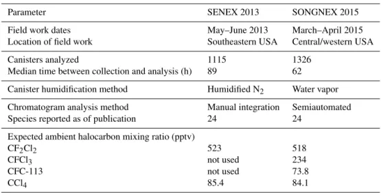
MSD
He
MFC
Vent
Vent
Vent
Vent
MF
C
MFC
Sample trap Water trap Vent
NaOH / SiO2 scrubber
MF
C
Std no. 1 Std no. 2
Col no. 2: DB-624
(Restek MXT-624)
Col no. 1: Al2O3/KCl
RT-Alumina BOND/ KCl PLOT
Vent
Vent
P
Column flush
Column flush
Channel 1 Channel 2
W
a
te
r
tra
p
f
lu
sh
Air sample
Helium
Processed air
Concentrated sample
Setting Import Setting Backflush Setting
Load
Setting Flush
Sample pressure P
Pump Vent Humidified zero air
Canister manifold pressure
Critical orifice
Sample canisters (racks no. 1– 3) Sample canisters (racks no. 4– 6)
3-way valve
2-way valve
Not used for canister analysis To ambient
inlet
Water trap
Sample trap
2– 10 2– 6
1– 10 1– 6
4 port
Figure 1.Schematic of instrument with flow path and valve position. Figure shown with open valve for a canister of middle-left sample module, Ch 1 flushing sample trap effluent to separation column, and Ch 2 loading sample trap.
sea level), fill time is typically 11 s, and the maximum fill time allowed by the flight computer is 15 s regardless of fill pressure. During SONGNEX 2015,≈95 % of samples were collected below 3500 m a.s.l. and had fill times between 3 and 7 s. At typical air speeds of 100 m s−1, these samples average the VOC composition over < 1 km of the flight track. The data system can be operated in a survey mode, whereby can-isters are automatically filled at set intervals (typically 180 to 450 s between samples). The flight scientist is also able to immediately collect sample(s) with an override function and can adjust the sample interval as required. Canister fill times are transmitted to the onboard flight scientist over the aircraft local area network and to scientists on the ground along with the aircraft GPS coordinates allowing for real-time mapping of sampling. When all canisters have filled, the sample man-ifold bypass valve is opened for venting and the compressor is turned off.
2.2 Post-flight analysis via GC-MS 2.2.1 Sampling from the canisters
Each canister is sequentially analyzed post-flight in the field with ACCBAR (Fig. 1). The canister modules are connected
valve is activated, allowing the sampling manifold to reach sufficient pressure to deliver sample flow (120 sccm) to the instrument through the orifice and to passivate the manifold surfaces with each sample prior to analysis. The GC-MS con-trol system evaluates the sample manifold pressure one sec-ond before opening the sample valve; if the manifold pres-sure is below 30 psia the GC-MS will automatically switch to an instrument zero to avoid sampling a vacuum (see below). This condition is typically met as a result of a canister that failed to fill during flight. If the manifold pressure is greater than 30 psia, the system will continue to flush the manifold and GC sample inlet for 35 s before sample acquisition is ini-tiated.
2.2.2 Sample analysis and description of GC-MS Conceptually, ACCBAR is a series of traps used to re-duce unwanted component(s) from the air sample matrix (i.e., water and carbon dioxide) while concentrating the tar-get analytes, which are subsequently injected on separation columns and detected via mass spectrometry on a 20 min cycle. The custom-built GC-MS ACCBAR consists of two channels, with channel 1 optimized for C2–C6 hydrocar-bons and halocarhydrocar-bons using a PLOT column and channel 2 optimized for C6–C10 hydrocarbons and oxygen- and nitrogen-containing species using a low- to mid-polarity phase column. A single quadrupole mass spectrometer de-tector (MSD) runs in selective ion mode for increased signal-to-noise response and sequentially analyzes the effluent from the two columns. This instrument is based on a two-channel GC-MS developed by NOAA Chemical Sciences Division and deployed on many field campaigns over the past 15 years (Gilman et al., 2013; Goldan et al., 1995). The new instru-ment is designed for field deployinstru-ment, capable of measur-ing in situ or analyzmeasur-ing canister samples, and is built into a 104 cm×104 cm×64 cm (H×W×D) rack shock-mounted
on casters. ACCBAR requires no cryogen (e.g., liquid nitro-gen), consuming only carrier gas (ultra-high purity He), cal-ibration gases (typically zero air and a secondary standard, discussed below) and 120 VAC power (2×15 A circuits).
The new GC-MS was successfully deployed in 2013 for SENEX to the Smyrna/Rutherford County Airport (Smyrna, TN) via a towable laboratory trailer which was parked in-side an aircraft hangar; for SONGNEX in 2015, ACCBAR remained in the CSD laboratory since field operations were predominantly from the nearby Rocky Mountain Metropoli-tan Airport (Broomfield, CO).
Figure 1 presents a schematic of the flow path of AC-CBAR, along with alternative settings of the five two-position chromatography valves (Valco, Vici Instruments, Houston, TX) used to direct gas flow. Channel 1 is shown with the 10-port valve (1–10) in “flush” mode and the 6-port valve (1–6) in “import” mode, where the sample trap is con-nected to the separation column with carrier gas (UHP He) flowing through the sample trap and to the column. Channel
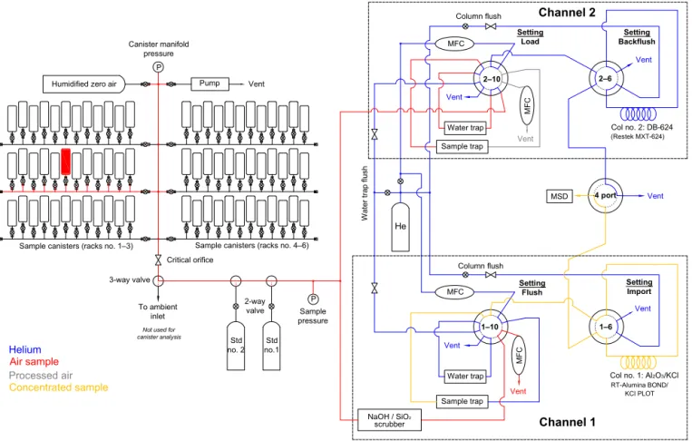
(a)
(b)
B
A
C
D
Sample in/out Flush gas in
Figure 2. (a)Drawing of ACCBAR sample trap (top view, side view). The cold block (A) is mounted inside a vacuum chamber (B), suspended upon two 3.2 mm OD stainless steel tubes (C). The Stirling cooler cold finger (not shown) bolts to the floating stage (D) centered above the cold block.(b)Temperature profile of Ch no. 2 sample trap at nominal−135◦C.
2 is shown with the 10-port valve (2–10) in “load” mode and the 6-port valve (2–6) in “backflush” mode, where sample flow is directed through a water trap followed by the sam-ple trap, while the separation column is isolated and back-flushed with UHP He. The four-port valve is shown direct-ing channel flow from the separation column on channel 1 to the mass spectrometer, while channel 2 flow (UHP He) is vented. All chromatography valves have stainless steel bod-ies with polyaryletherketone/PTFE rotors with 0.40 mm di-ameter channel, without external purging. The valves and transfer lines (Restek, 1/16 in. OD Sulfinert-treated stainless steel) are housed within an oven that is held at a constant 80◦C.
condition must be avoided. Carbon dioxide (CO2), which can freeze and plug the channel 1 sample trap at collection temperature, must be removed. The channel 1 sample passes through a bed of heated (35◦C) granular NaOH-coated sil-ica (Ascarite II) packed in a 10 cm PFA tube (6.3 mm ID) with silanized borosilicate wool at each end (Goldan et al., 2004). No CO2trap is required for channel 2, as the sample trap temperature is just warm enough to prevent freezing of CO2at the residence time of the trap. Water vapor also must be removed from the air samples to prevent ice buildup in the subsequent sample traps, which would cause plugged flow, as well as to prevent degradation of the PLOT column used for channel 1. Prior to sample trapping, the air aliquot for each channel passes through a water trap, which is a 36 cm loop of 2.0 mm ID PEEK tubing inside a coaxial stainless steel tube resistively heated to control temperature, mounted in an insulated aluminum cold block. The water traps are cooled to−20◦C during trapping and then are heated to 100◦C for 12.9 min between sample injections while being backflushed with UHP He. The water trap cold block is chilled with a single-stage mechanical refrigerator (Neslab, model CC-65) during operation. The water traps are able to cool from purge to trapping temperature in approximately 45 s and are con-trolled within 0.2◦C of set point during trapping.
After passing through the water traps, analytes from the air samples are pre-concentrated via cryogenic trapping at nominal temperatures of−165 and−135◦C for channels 1
and 2, respectively. The sample traps (Fig. 2a) are a novel design, using a Stirling cooler (Sunpower Inc., Athens, OH, model CryoTel GT) to achieve trapping temperatures with-out the need for liquid nitrogen. The CryoTel GT cooler is capable of 16W lift capacity (e.g., heat removal) at
−196◦C at maximum power (240W input) while weigh-ing only 3.1 kg. The cold end of the cooler terminates in a threaded cold finger, which is bolted to a small copper plate (25 mm×25 mm×6 mm) that is attached to a larger
cop-per cold block (178 mm×51 mm×10 mm) via 12 stranded
copper wires (10 AWG). This serves to mechanically isolate the cold finger from the cold block while still allowing effi-cient thermal transfer. The copper cold block is mounted in a 20 cm ID×6.2 cm cylindrical vacuum chamber, suspended
by two 3.2 mm OD, 2.7 mm ID stainless steel tubes that are sealed with Swagelok Ultra-Torr fittings. The Stirling cooler is mounted to the top of the chamber via a KF-50 vacuum flange attached to the cooler at the terminus end of the cold finger, and a turbomolecular pump is mounted to the bottom of the chamber to reduce pressure inside the chamber below 1×10⁻⁴hPa. The vacuum chamber has additional ports to allow for pressure measurement and sensor and heater wiring to the cold block.
The sample traps consist of a 330 mm section of treated fused silica tubing (0.53 mm ID) mounted inside a thin-wall hypodermic stainless steel tube (0.97 mm ID, 1.08 mm OD) that is resistively heated. The treated fused silica tubing used for channel 1 is Al2O3/KCl PLOT column (Restek
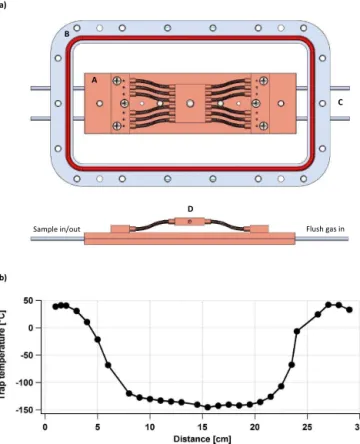
RT-Figure 3. (a)Valve positions and temperature profile of sample traps for an analysis cycle. The 10-port valves control flow to the water and sample traps, the 6-port valves control flow to the sep-aration columns and the 4-port valve controls flow to the detector. (b)For Ch no. 1 trap, the exponential rate of cooling≈8.4 s and the trap is cooled from 100 to−165◦C in 25 s.(c)For Ch no. 2 trap, the exponential rate of cooling≈7.0 s and the trap is cooled from 100 to−135◦C in 18 s.
Alumina BOND/KCl), with the Al2O3 scraped from each end of the tubing so that only the center 180 mm is coated; channel 2 uses deactivated fused silica (Restek Rxi Guard) without modification. To allow temperature control of the sample trap, a type-T thermocouple is adhered to the outer wall of the hypodermic tubing with shrink tubing, which electrically isolates the heater from the outer support tubing. The ends of the hypodermic tubing – that part of the heater tubing that is not positioned inside the cold block – are plated with 30 µm copper then flashed with gold to reduce the re-sistance of the heaters at the ends; this avoids overheating the ends of the sample trap while controlling the tempera-ture in the center (Fig. 2b). The trap assemblies are installed inside the 3.2 mm OD stainless steel support tubes described above. During typical operation throughout the sample cycle, the Stirling cooler is operated at 220W rather than full power, as this is adequate to maintain an average cold block temper-ature of−180◦C. At maximum cooler power, it is possible to
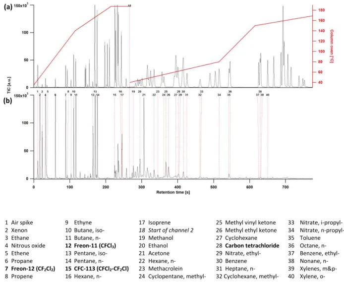
1 Air spike 9 Ethyne 17 Isoprene 25 Methyl vinyl ketone 33 Nitrate, i-propyl-
2 Xenon 10 Butane, iso- 18 Start of channel 2 26 Methyl ethyl ketone 34 Nitrate, n-propyl-
3 Ethane 11 Butane, n- 19 Methanol 27 Cyclohexane 35 Toluene
4 Nitrous oxide 12 Freon-11 (CFCl3) 20 Ethanol 28 Carbon tetrachloride 36 Octane, n-
5 Ethene 13 Pentane, iso- 21 Acetone 29 Nitrate, ethyl- 37 Benzene, ethyl-
6 Propane 14 Pentane, n- 22 Hexane, n- 30 Benzene 38 Nonane, n-
7 Freon-12 (CF2Cl2) 15 CFC-113 (CFCl2-CF2Cl) 23 Methacrolein 31 Heptane, n- 39 Xylenes, m&p-
8 Propene 16 Hexane, n- 24 Cyclopentane, methyl- 32 Cyclohexane, methyl- 40 Xylene, o-
(a)
(b)
Figure 4.Chromatograms displayed as total ion current (TIC) with select peaks identified. Top panel(a)shows secondary standard, along with temperature ramp for each GC channel. Bottom panel(b)shows air sample collected in the Haynesville oil and gas field near Shreveport, Louisiana, 25 April 2015.
Fig. 3a shows a typical temperature trace for each sample trap during an analytical cycle. At cycle time (t)=0 s, the traps are held at temperatures slightly above trapping tem-peratures (−120 and−100◦C for channel 1 and 2, respec-tively) while being backflushed with UHP He to reduce the heat load to the Stirling cooler between sampling periods. Before sample trapping begins, both traps are heated sequen-tially to > 100◦C (att=105 and t=135 s for channels 1
and 2, respectively) and held at this temperature for 20 s to ensure the traps are as clean as possible, then cooled to their trapping temperatures (−165 and−135◦C for channel 1 and
2, respectively). The heater design allows for rapid heating and cooling of the sample traps, so the traps can switch from cold to hot set point temperatures in less than 3 s and can be cooled from 100◦C to their respective trapping temperatures in less than 30 s (Fig. 3b and c). The novel geometry of the sample trap and the duty cycles of the heaters allows for this
performance, while operating within the constraints of the lifting power of the Stirling cooler.
Sample flow is directed to both traps starting att=210 s by switching the 10-port valves from “flush” to “load” posi-tion which is maintained for 240 s at a flow rate of 60 sccm; during sample collection, the sample trap temperature is con-trolled to within 0.2◦C by heating. Att=450 s, the 10-port
valves simultaneously switch back to the “flush” position stopping sample flow to the traps, which are then backflushed with UHP He while maintaining trapping temperatures. This post-collection flush removes most of the untrapped perma-nent gases (e.g., nitrogen, oxygen, argon) from the sample trap flow path, thereby reducing the chromatogram back-ground signal at the start of each channel. The sample traps are flash-heated att=553 andt=796 s of the cycle
and is injected onto the column quickly/efficiently enough so that no cryofocus is required on the column heads.
After trapping, the concentrated samples are injected in turn onto the respective chromatography columns. UHP He is used as the carrier gas, at a constant flow of 2 sccm, with the total chromatogram requiring 780 s of run time. After separa-tion, the column effluent is directed sequentially to the MSD via a four-port valve (Fig. 1), with channel 1 measured first, followed by channel 2. Channel 1 uses an Al2O3/KCl PLOT column (Restek RT-Alumina BOND/KCl; 30 m length, 0.25 mm ID, 4 µm film thickness), with a temperature profile ramped from 35 to 190◦C in 190 s. Channel 2 uses a low-to mid-polarity modified methylpolysiloxane (Restek MXT-624; 30 m length, 0.25 mm ID, 1.4 µm film thickness), with a temperature profile ramped from 40 to 170◦C in 518 s. For both columns, the temperature programs are multi-step ramps with several different heating rates used to optimize peak separation for each column (Fig. 4a). The columns are individually sheathed inside two custom interlocking alu-minum spindles (12.2 cm OD, 10.5 cm ID). The columns are wrapped around the innermost spindle along with resis-tive temperature detectors (RTDs) for temperature measure-ment. The spindles are heated resistively with Kapton thin-film heaters. Both spindles are suspended inside fiberglass housings by thin (0.38 mm) stainless steel tabs. The hous-ings have 150×172 mm fans mounted on one side to cool
the columns; the fans are operated by pulse-wave modula-tion and can be reduced to≈40 % power, allowing for low
air flow rates across the heated column spindles and thereby improving temperature control at temperatures close to ambi-ent. After each column has completed separation, it is back-flushed with UHP He while heated to 190 or 210◦C for chan-nel 1 and 2, respectively, before cooling in preparation for the next sample.
The mass spectrometer (Agilent model 5975C) is usu-ally operated in selected ion monitoring mode, scanning up to 11 masses per window, 28 windows per chromatogram with dwell times between 10 and 20 ms per mass, to opti-mize instrument sensitivity while providing enough sample points per mass to accurately determine peak area. Beginning with the 2015 SONGNEX campaign, a new peak-integration software package called TERN (Aerodyne Research, Inc.) has been used for automated peak-area retrieval (Isaacman-VanWertz et al., 2017). TERN is a custom-designed chro-matographic data handler and peak integration package built upon Igor Pro’s (Wavemetrics, Inc.) multi-peak fitting func-tionality. Chromatographic peaks are fit by minimizing the residual of a set of Gaussian and exponentially modified Gaussian peaks for a subset of the chromatogram (typically 20 s) on a single mass. The peak within this optimized fit considered most likely to be the analyte of interest is re-turned, and the peak area is calculated from the coefficients of the solution. Use of TERN to integrate chromatograms has reduced analysis time to approximately 1.25 min per chro-matogram, at least an order of magnitude faster than the
previous method using Agilent ChemStation and hand inte-gration, while increasing peak area precision and accuracy (Isaacman-VanWertz et al., 2017). Additional information about TERN’s peak fitting method and an intercomparison between peak areas determined by manual integration and automatic peak fitting is provided in the Supplement. 2.2.3 Canister cleaning and conditioning
After the canisters have been analyzed, they must be prepared and conditioned for reuse. An automated cleaning oven has been constructed that allows for the unattended processing of three canister modules at one time. All tubing and fittings in the oven are stainless steel. Each canister manifold, and then each individual canister, is evacuated and leak-tested. The canisters are then heated to 65◦C under vacuum using a dry scroll pump for 1 h, typically to less than 0.01 hPa as measured between the canister modules and the pump. Canisters are then filled with humidified high-purity nitrogen gas (UHP N2or liquid nitrogen blow-off) and re-evacuated. The nitrogen flush and pump out process is repeated a min-imum of three times. After the final canister pump down, approximately 15 hPa of water vapor is added to the canis-ters to reduce artifacts in the subsequent air sample collected in the canisters (Ochiai et al., 2002). Water for both nitro-gen humidification and water vapor addition is HPLC-grade (Sigma-Aldrich), in a bubbler heated to nominally 35◦C. Af-ter the final evacuation step of the cleaning cycle, all sam-ple canisters are opened for 2.5 min in order to be filled to
∼15 hPa with water vapor. This is done by shutting off the nitrogen flow to the water bubbler so that only the headspace over the water reservoir is available to fill the evacuated can-isters with water vapor. Water is delivered to the cancan-isters via stainless steel tubing. The final fill pressure varied by less than 5 % for each campaign. The cleaning and humidifica-tion procedure is based upon a survey of canister preparahumidifica-tion methods presented in the literature (Colman et al., 2001; Mc-Clenny et al., 1991; Plass-Dülmer et al., 2006; WMO, 2012), albeit at a slightly lower bake-out temperature than the range cited (70–80◦C). After the SONGNEX field campaign, the cleaning oven was rebuilt to operate at 75◦C.
am-bient water mixing ratios of the collected samples from each field campaign is described in the Supplement. During a field campaign, the efficacy of the cleaning system is evaluated by filling cleaned and humidified canisters with the same zero air gas used to test for artifacts (Sect. 3.4.2).
3 Results: normalization, calibration, artifacts 3.1 Normalization of instrument response
For both chromatograph channels, normalization is required to account for changes in instrument sensitivity primar-ily attributable to changes in detector response. Long-lived halocarbon species in the atmosphere are used for normal-ization, effectively serving as internal standards for can-ister samples (Karbiwnyk et al., 2003). Four halocarbons have been selected (only two were used for SENEX), which are abundant and relatively constant in tropo-spheric air as a function of latitude over the typical one-month time period of a field campaign: Freon-12 (CF2Cl2, dichlorodifluoromethane), Freon-11 (CFCl3, trichlorofluo-romethane), CFC-113 (CFCl2–CF2Cl, 1,1,2-trichloro-1,2,2-trifluoroethane) and carbon tetrachloride (CCl4, tetra-chloromethane). Expected mixing ratios in ambient air for each halocarbon (Table 1) are estimated from data provided by the NOAA Global Monitoring Division using averaged monthly data from the nearest sampling sites by latitude: Niwot Ridge, CO, and Trinidad Head, CA (Montzka et al., 2015). These halocarbons are also added quantitatively to a custom dilution of a 57-component ozone precursor hydro-carbon standard (Scott Specialty Gases) in UHP nitrogen. The mixing ratio of the secondary standard is 275 pptv for all hydrocarbons with 7 % uncertainty for each compound. The secondary standard also contains the halocarbons used for normalization at the following mixing ratios with 6 % uncertainty: CF2Cl2=140, CFCl3=26.2, CFC-113=12.0 and CCl4=87.5 pptv. This gas mixture serves as a single-point secondary standard during field measurements to char-acterize instrument response throughout the campaign. The secondary standard is also measured periodically during sen-sitivity studies (Sect. 3.2), as the analyte consists of stan-dard(s) diluted in UHP nitrogen and therefore has no sig-nificant halocarbon mixing ratios. This allows for quantifi-cation of normalization factors in both ambient samples and calibration samples. An example time series for the raw in-strument response for a halocarbon and hydrocarbon species in the secondary standard measured on each channel is pro-vided in the Supplement (Fig. S4).
A normalization factor is calculated for every sample, based on the raw peak area for CF2Cl2on channel 1 (CFCl3 and CFC-113 were also used for SONGNEX, see below), and CCl4 on channel 2. The calculation of a normalization factor (NF) is shown in Eq. (1):
NF=Rawhalo/Targethalo. (1)
Here, halo is a halocarbon used for normalization, Raw is the integrated raw counts for a peak and Target is the expected raw counts. The secondary standard has a CCl4mixing ratio of 87.5 pptv, with a target response of 15 000 counts; during SONGNEX an ambient mixing ratio of 84.1 pptv as reported by NOAA GMD, and a target response of 14 400 counts was assumed. For SENEX, a single normalization factor was cal-culated for each channel using Eq. (1). For SONGNEX, three normalization factors (NFhalo)were calculated for channel 1 from halocarbon responses spanning that channel’s elution time (Fig. 4). The final normalization factor was then cal-culated by linear interpolation, based upon the target ana-lyte retention time (Eq. 2); for species eluting outside these halocarbon retention times, the nearest halocarbon factor was used.
NFsp=Rawsp/NFhalo2− NFhalo2−NFhalo1
× RThalo2−RTsp
/ RThalo2−RThalo1
(2) Here, sp is the analyte species of interest, halo1 and halo2 are the halocarbons eluting before and after the analyte, re-spectively, and RT is retention time. The additional step of fitting multiple halocarbons was performed for channel 1 to account for some additional sensitivity changes independent of the detector response, which may be related to changes in trapping efficiency of the PLOT material in the sample trap. Peak areas are reported as normalized kilocounts (nkcts) sim-ply by dividing the raw peak area by the relevant NF. This method is applied to all samples with known mixing ratios of these halocarbons, either from standards or ambient air, rather than interpolating only between standards in order to improve the accuracy of the normalization. For samples with no or unknown mixing ratios of halocarbons (e.g., instrument zeros, sensitivity calibrations), the normalization factors are interpolated from ambient and calibration samples.
3.2 Calibration
and 40 % for all data points. The analyte flow is controlled at multiple setpoints between 0.3 and 3 sccm with the low flow MFC, while crimped capillaries allow constant flow within the same range. Flows are measured using DryCal flow me-ters for dilution flows and a soap bubble flow meter for ana-lyte flows. All tubing used in the dynamic dilution system is 6.2 mm OD PFA, and a 10 m loop of PFA tubing is placed be-tween the dilution system and instrument to ensure adequate mixing before sampling.
Typically, at least seven dilution levels are sampled over at least 3 orders of magnitude; for SONGNEX, this range was 0.03–70 ppbv. Hydrocarbon calibrations are performed with a nominal 1 ppm PAMS 57-component commercial standard (Scott Specialty), with a stated 5 % uncertainty of individual component concentrations. Other species – oxygenated com-pounds, alkyl nitrates, monoterpenes – are calibrated with in-house-made gravimetric standards consisting of 1–10 ppm mixtures of up to 10 species, with 5 % uncertainties. In-house standards include at least two hydrocarbons also found in the PAMS standard, typically benzene or toluene, in order to confirm that instrument response is consistent across a series of calibration tests. Secondary gas standards are exchanged and analyzed with the NOAA Global Monitoring Division (GMD) Halocarbons and other Atmospheric Trace Species (HATS) group on an informal basis every 1 to 2 years to es-tablish the veracity of the stated gas standard concentrations. This process led to the discovery of the misstated ethane mix-ing ratio in our current primary PAMS standard (14 % higher than stated). Accounting for additional measurement errors of flows of the dynamic dilution system, 1 % for analyte and 2 % for dilution, we define the calibration accuracy as the uncertainties of concentration and flow added in quadrature. These values are listed in Table 2. We have left the larger uncertainty in ethane accuracy in our current description of the GC-MS performance, as we are continuing to evaluate ethane standards.
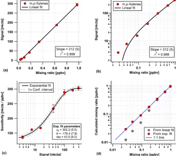
Instrument responses for most compounds are nonlinear over the dynamic range of the calibrations. This behavior is consistent with what has been observed on this laboratory’s previous GC-MS system, although the nonlinear response on the previous generation of this instrument was only signifi-cant for later eluting compounds (those after benzene). When plotted with linear-log scaling, the behavior is sigmoidal, in that sensitivity is constant at low mixing ratios, then transi-tions to a higher sensitivity at high mixing ratios. The sensi-tivity can be described well with an exponential function: Sens=Sens0+A/e(
τ
nct), (3)
where Sens is the sensitivity at a given normalized count sig-nal (nct), Sens0 is the sensitivity at low mixing ratios, A is the difference in sensitivity between low and high mix-ing ratios and τ is the normalized count signal midway be-tween low and high sensitivity. An example of solving for the nonlinear sensitivity (for m, p-xylenes) is presented in
Fig. 5, where a seven-point calibration curve is shown span-ning 0.025–1.0 ppbv mixing ratio. The linear fit statistics for the data points indicate a very good fit (Fig. 5a), with a small uncertainty of the slope (< 2 %) andr2=0.999. However, re-plotting the data on a log–log scale (Fig. 5b) shows that the fit does a poor job describing the data collected at the lowest mixing ratios. Solving for individual sensitivities at each cal-ibration mixing ratio, simply by dividing normalized counts by mixing ratio and plotting versus normalized counts on a logarithmic, shows the sigmoidal behavior described above (Fig. 5c). These data are described well with Eq. (3), and comparing calculated mixing ratios found with the linear and nonlinear sensitivities (Fig. 5d) shows that the nonlinear sen-sitivity provides an excellent match across the entire dynamic range of the calibration. We also provide a measure for the nonlinearity, using the ratio of A : Sens0, for all species re-ported in Table 2; for the earliest eluting compounds no non-linearity is observed.
This behavior is the opposite of what is typically observed when analyte breakthrough occurs at the sample trap, and we have tested the instrument up to 180 ppbv with a mix-ture of light hydrocarbons most susceptible to breakthrough (ethane, ethene, propane, propene, ethyne, n-butane) with no observed decrease in sensitivity; this mixing ratio is larger than any we have observed in ambient air with the WAS sys-tem. The nonlinearity is currently attributed to the water trap. At high mixing ratios the gas-phase analyte reaches equilib-rium with adsorbed analyte on the wetted surfaces of the wa-ter trap, while at low mixing ratios this equilibrium is never reached and losses are kinetically determined. Precise con-trol of the water trap temperature and sample flow rate are required to ensure that the nonlinearity is reproducible. Al-ternative water trap geometries and materials are currently under investigation to reduce this nonlinearity.
3.3 Precision, limits of detection and total analysis uncertainty
preci-Table 2.VOC species measured by iWAS/ACCBAR during SONGNEX. For each compound, the instrument channel, nonlinearity (Nonlin.; as described in the text, the ratio A : Sens0), calibration standard accuracy (Cal acc.), calibration fit uncertainty (Fit unc.), precision and total
uncertainty (Total Unc.) are reported.
Compound Channel Nonlin. Cal acc. Fit unc. Precision Total Unc.
(%) (%) (%) (%±pptv)
Ethane 1 – 15 3.5 8 17+0.6
Propane 1 – 6 2.1 6 9+3
i-Butane 1 0.19 6 2.4 5 8+1
n-Butane 1 0.23 6 2.3 5 8+0.8
i-Pentane 1 0.33 6 1.6 3 7+0.8
n-Pentane 1 0.33 6 2.3 3 7+0.8
n-Hexane 1 0.34 6 3.9 4 8+5
n-Hexane 2 0.31 6 1.3 3 7+1
n-Heptane 2 0.39 6 2.5 4 8+0.8
n-Octane 2 0.53 6 2.0 3 7+1
n-Nonane 2 0.64 6 3.4 5 9+2
Ethene 1 – 6 3.4 8 11+3
Isoprene 1 0.32 6 3.5 7 10+3
αPinene 2 0.64 6 2.8 1 7+1
βPinene 2 0.64 6 6.9 1 9+2
Ethyne 1 0.16 6 1.7 5 8+0.5
Methylcyclopentane 2 6 3 7
Cyclohexane 2 0.29 6 1.4 4 7+2
Methylcyclohexane 2 0.44 6 2.7 5 8+1
Benzene 2 0.20 6 1.3 2 6+0.6
Toluene 2 0.34 6 3.0 4 8+2
Ethylbenzene 2 0.54 6 3.1 6 9+1
m, p-Xylenes 2 0.59 6 3.5 2 7+1
o-Xylene 2 0.52 6 2.8 4 8+1
Nitrate, ethyl 2 0.32 6 6.6 2 9+4
Nitrate, i-propyl 2 0.38 6 5.8 2 9+3
Nitrate, n-propyl 2 0.38 6 6.0 2 9+4
Methanol 2 0.49 6 3.0 4 8+15
Ethanol 2 0.77 6 1.8 4 7+12
Acetone 2 0.22 6 0.9 2 6+5
Methyl ethyl ketone 2 0.25 6 0.4 1 6+3
Methyl vinyl ketone 2 0.27 6 0.8 2 6+5
Acetaldehyde 2 0.32 6 3.6 3 8+8
Propanal 2 – 6 1.6 2 7+3
Methacrolein 2 0.30 6 0.6 2 6+3
sion estimate and the instrument sensitivity:
DL=3×σprec×Sens, (4)
where σprec is the standard deviation of the lowest cali-bration point (minimum four replicates) for any reported species in units of nkcts and Sens is the instrument sensi-tivity for that species, in units of pptv nkct−1 (Oliver et al., 1996). An example chromatogram is shown in the Supple-ment (Fig. S4) for a calibration measureSupple-ment at 26 pptv mix-ing ratio of the 57-component PAMS mixture described in Sect. 3.2. For most species, the detection limit is less than or equal to 5 pptv and often below 1 pptv, but ACCBAR had significantly higher limits of detection for several oxygenated species. The humidification system used during dynamic
di-lutions contributes significant backgrounds for some oxy-genated species (e.g., alcohols) and thereby increasing the standard deviation of those calibration points. Total analytic uncertainty for each reported species is the sum in quadrature of the uncertainties of the calibration standard and sensitiv-ity function and the precision. Total uncertainty must also account for absolute uncertainty at low mixing ratios as the DL, so that our total uncertainty is stated as relative uncer-tainty (%)+absolute uncertainty (pptv). Total uncertainty
Figure 5.Example nonlinear sensitivity calibration for m, p-xylenes. Panels(a)and(b)show a linear fit of normalized signal versus mixing ratio for a seven-point calibration, using linear and log scaling of the same data. In panel(c)an exponential function has been fit to sensitivity calculated at each calibration point versus normalized counts. Panel(d) shows mixing ratio calculated from both the linear fit and the exponential fit of sensitivity plotted against actual mixing ratio. Values in parentheses are 1σuncertainties of fit coefficients.
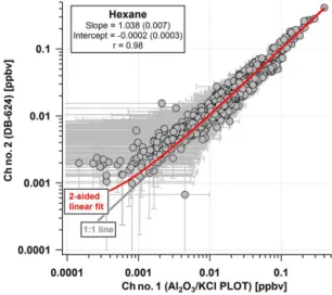
To assess the overall analytical uncertainty further, the measurements of n-hexane, which is quantified on both chan-nels of the GC-MS, are compared. Figure 6 shows a scatter plot of n-hexane measurements for the entire SENEX field campaign. The two-sided linear fit of the data indicates an agreement within 4 % with an insignificant intercept and lit-tle scatter (a least-squares fit gives a correlation coefficient,
r, of 0.98).
3.4 Sample canister tests
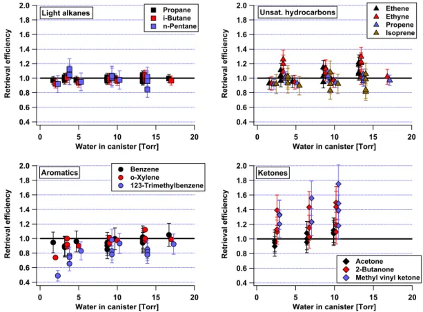
Previous work (Kelly and Holdren, 1995; Ochiai et al., 2002; Palluau et al., 2005) has indicated that samples collected in dry electropolished stainless steel canisters may be subject to significant artifacts due to loss of certain VOCs to the canister walls, while samples humidified either via addition of water prior to sampling or by adequate ambient water vapor will be less prone to these effects. The iWAS/ACCBAR system was evaluated for potential artifacts due to canister preparation, sample collection and sample aging. This was accomplished via four sets of tests.
3.4.1 Canister humidification and retrieval efficiency
A series of humidification experiments were performed using ambient air samples collected outside the laboratory in Boul-der, CO, in canisters filled with varying amounts of water vapor after the cleaning process (Fig. 7). The goal of these tests was to determine the minimum level of water vapor that should be added to the sample canisters in order to suf-ficiently reduce analyte losses to the canister surfaces. AC-CBAR collected and measured the ambient air in situ while canister were simultaneously filled, using a common PFA in-let for both systems. Ambient dew points during these tests varied between−1 and 5◦C (15–40 % RH), while air
Figure 6.Intercomparison of n-hexane measurements made by the two different channels of iWAS/ACCBAR system during SENEX 2013. Data are shown with error bars based upon total analytical uncertainty presented in Table 2.
for samples collected at approximately the same time. Rtv Eff=mean concentration canister/
mean concentration in situ (5)
Most hydrocarbons show retrieval efficiencies near unity, with considerable scatter due to the difficulty in comparing a 4 min integrated sample (in situ) with a 30 s integrated sample (canister). For most species, water vapor pressure > 10 torr (13 hPa) was found to be adequate to passivate the canisters, although heavy aromatics (> C8) showed signif-icant losses at all levels. Ketones are positively correlated with added water, indicating a possible contamination with the canister humidification system.
3.4.2 Canister blanks
During SONGNEX, the sampling system was evaluated for background signal by filling canisters with zero air immedi-ately after cleaning and humidifying, then allowing the cans to sit 1–3 days before analysis. These tests are in contrast to the analysis system blanks (see Sect. 2.2.1) as they iden-tify signal enhancements attributable to canister preparation. These results are presented in Table 3 as blanks in units of pptv. Hydrocarbons and alkyl nitrates have very small sig-nals in the blanks, with ethane being the only species with a mixing ratio greater than 2 pptv. However, a few oxygenated species had blank values at atmospherically relevant levels. The blanks were significantly larger than the analysis sys-tem blanks (the same zero air passed through the sample train) so the artifacts are attributed to the canisters rather than the analysis system. Since nearly all species but oxygenates were below detection limit, the canister cleaning appears to be adequate. Instead, the source of contamination is likely
the canister humidification system, confirming the observa-tions noted in Sect. 3.4.1. Because of this contamination, oxygenates are not reported for SONGNEX. For SENEX, sample canisters were pre-treated not with water vapor but with humidified nitrogen (see Sect. 2.2.3), so mixing ratios of oxygenates collected in the planetary boundary layer are ex-pected to be less perturbed for this dataset. Also note that dur-ing SONGNEX, ACCBAR showed a significant ethanol con-tamination that decayed exponentially throughout the cam-paign, so that the reported ethanol blank value here is likely a combination of instrument and canister artifact.
3.4.3 Canister aging and retrieval efficiency
2.0 1.8 1.6 1.4 1.2 1.0 0.8 0.6 0.4 Retri eval effi ci en cy 20 15 10 5 0
Water in canister [Torr]
Acetone 2-Butanone Methyl vinyl ketone
Ketones 2.0 1.8 1.6 1.4 1.2 1.0 0.8 0.6 0.4 Retri eval effi ci en cy 20 15 10 5 0
Water in canister [Torr]
Ethene Ethyne Propene Isoprene Unsat. hydrocarbons 2.0 1.8 1.6 1.4 1.2 1.0 0.8 0.6 0.4 Retri eval effi ci en cy 20 15 10 5 0
Water in canister [Torr]
Aromatics Benzene
o-Xylene 123-Trimethylbenzene 2.0 1.8 1.6 1.4 1.2 1.0 0.8 0.6 0.4 Retri eval effi ci en cy 20 15 10 5 0
Water in canister [Torr]
Propane i-Butane n-Pentane
Light alkanes
Figure 7.Retrieval efficiency as a function of added water vapor to sample canisters after cleaning. Data points are the ratio of observed mixing ratios in canister samples versus ambient mixing ratios measured by ACCBAR during the time period the canisters were filled. Error bars indicate standard deviation of multiple canisters filled simultaneously. Data are offset onxaxis for easier viewing.
0.45 0.40 0.35 0.30 0.25 0.20 Can samp le [p p b v] 0.45 0.40 0.35 0.30 0.25 0.20
Ambient sample [ppbv]
Ethyne Slope = 1.02 ± 0.13 Intercept = -0.18 ± 1.21
r = 0.93
Days after spl collection
One Two Four
1:1 line 0.5 0.4 0.3 0.2 Can samp le [p p b v] 0.45 0.40 0.35 0.30 0.25 0.20 0.15
Ambient sample [ppbv]
Toluene Slope = 0.87 ± 0.06 Intercept = -1.2 ± 4.9
r = 0.96
Figure 8.Canister samples versus in situ ambient samples collected in Boulder, CO, using sample canisters humidified to 12 torr water vapor during the cleaning process. Error bars indicate standard deviation of replicate canister samples.
3.4.4 Canister replicates
During SONGNEX replicate analysis was performed on full sets of canister samples from three research flights to evalu-ate the analytical precision of the entire system (rather than just the GC-MS). The research flights were made on 9 April through the eastern Permian Basin of Texas, on 13 April in the Denver–Julesburg Basin and Colorado Front Range and on 23 April through the western Permian Basin of Texas and
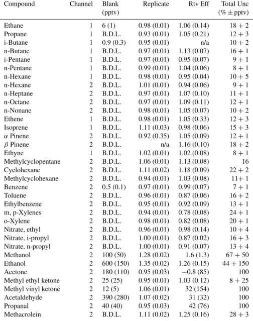
Repli-Table 3.VOC species measured by iWAS/ACCBAR during SONGNEX. Canister backgrounds (Blank), replicates and retrieval efficiencies (Rtv Eff) and total uncertainties are reported. Replicate compares two analyses of the same sample canister performed within 100 h of each other. Retrieval efficiency (Rtv Eff) is the ratio of the observed mixing ratio between canister and in situ samples collected simultaneously, with the canisters then analyzed within 100 h of collection. Total uncertainty is reported as %+pptv.
Compound Channel Blank Replicate Rtv Eff Total Unc
(pptv) (%±pptv)
Ethane 1 6 (1) 0.98 (0.01) 1.06 (0.14) 18+2
Propane 1 B.D.L. 0.93 (0.01) 1.05 (0.21) 12+3
i-Butane 1 0.9 (0.3) 0.95 (0.01) n/a 10+2
n-Butane 1 B.D.L. 0.97 (0.01) 1.13 (0.07) 16+1
i-Pentane 1 B.D.L. 0.97 (0.01) 0.95 (0.07) 9+1
n-Pentane 1 B.D.L. 0.99 (0.01) 1.04 (0.06) 8+1
n-Hexane 1 B.D.L. 0.98 (0.01) 0.95 (0.04) 10+5
n-Hexane 2 B.D.L. 1.01 (0.01) 0.94 (0.06) 9+1
n-Heptane 2 B.D.L. 0.97 (0.01) 1.07 (0.10) 11+1
n-Octane 2 B.D.L. 0.97 (0.01) 1.09 (0.11) 12+1
n-Nonane 2 B.D.L. 0.98 (0.01) 1.05 (0.07) 10+2
Ethene 1 B.D.L. 0.98 (0.01) 1.05 (0.33) 12+3
Isoprene 1 B.D.L. 1.11 (0.03) 0.98 (0.06) 15+3
αPinene 2 B.D.L. 0.92 (0.35) 1.05 (0.09) 12+1
βPinene 2 B.D.L. n/a 1.16 (0.10) 18+2
Ethyne 1 B.D.L. 1.02 (0.01) 1.02 (0.08) 8+1
Methylcyclopentane 2 B.D.L. 1.06 (0.01) 1.13 (0.08) 16
Cyclohexane 2 B.D.L. 1.11 (0.02) 1.18 (0.09) 22+2
Methylcyclohexane 2 B.D.L. 0.94 (0.01) 1.03 (0.08) 11+1
Benzene 2 0.5 (0.1) 0.97 (0.01) 0.99 (0.07) 7+1
Toluene 2 B.D.L. 0.96 (0.01) 0.87 (0.06) 16+2
Ethylbenzene 2 B.D.L. 0.95 (0.01) 0.92 (0.09) 13+1
m, p-Xylenes 2 B.D.L. 0.94 (0.01) 0.78 (0.08) 24+1
o-Xylene 2 B.D.L. 0.98 (0.01) 0.82 (0.08) 20+1
Nitrate, ethyl 2 B.D.L. 0.96 (0.01) 0.98 (0.14) 10+4
Nitrate, i-propyl 2 B.D.L. 1.00 (0.01) 0.87 (0.02) 16+3
Nitrate, n-propyl 2 B.D.L. 1.00 (0.01) 0.91 (0.07) 13+4
Methanol 2 100 (50) 1.28 (0.02) 1.6 (1.3) 67+50
Ethanol 2 600 (150) 1.35 (0.02) 1.26 (0.15) 44+150
Acetone 2 180 (110) 0.95 (0.03) −0.8 (85) 100
Methyl ethyl ketone 2 25 (25) 0.95 (0.01) 1.03 (0.12) 8+25
Methyl vinyl ketone 2 12 (5) 1.06 (0.01) 32 (154) 100
Acetaldehyde 2 390 (280) 1.07 (0.02) 31 (32) 100
Propanal 2 40 (40) 0.95 (0.03) 42 (76) 100
Methacrolein 2 B.D.L. 1.11 (0.02) 1.25 (0.16) 28+3
cate results for aldehyde and ketone species typically agreed within 10 %, indicating that the analysis system does not con-tribute measurement artifacts for these species. For cans aged 256 h on average, several additional classes of compounds (ketones, alkyl nitrates, aromatics) showed enhancements in the second analysis. For SONGNEX, most canisters (92 %) were analyzed within 100 h of sampling, so only the 37 and 92 h replicate results are considered to be applicable here. The results of these tests are summarized in Table 3 as the slope of the two-sided linear regression of the combined 37 and 92 h replicates, ignoring the 256 h replicate samples.
3.4.5 Total uncertainty
Using the information from the canister tests and the total analytical uncertainty reported in Sect. 3.3, we can describe the total uncertainty for measurements reported from the iWAS/ACCBAR system for SONGNEX, reported as relative plus absolute uncertainty (%+pptv). For each compound,
7 1
2 3 4 5 6 7 10
2 3 4 5 6 7 100 First analysis [ppbv]
Ethane 250 200 150 100 50
Time between replicates [h]
1:1 line 0.001 2 4 6 0.01 2 4 6 0.1 2 4 Rep li cate [p p b v] 8 0.001
2 4 6 8 0.01
2 4 6 8 0.1
2 4
First analysis [ppbv] Toluene 2 3 4 5 6 0.01 2 3 4 5 6 0.1 Rep li cate [p p b v]
2 3 4 5 6 7 8 9 0.01
2 3 4 5 6 7 8 9 0.1 First analysis [ppbv]
Nitrate, i-propyl
Figure 9.Comparison of replicate analyses from the same sample canister sets from three flights during SONGNEX 2015 (flight dates: 9, 13, 23 April).
tween 10 and 20 % for hydrocarbons and alkyl nitrates. Dur-ing SONGNEX, most oxygenated species had significantly larger uncertainties due to uncertain retrieval efficiencies, with only methyl ethyl ketone and methacrolein having ac-ceptable uncertainty levels. Further canister testing evalua-tions are required to determine if improved canister prepa-ration and handling will allow for reduced uncertainties of oxygenated species.
4 Results: measurement validation by intercomparison with other measurements
4.1 SENEX 2013
The iWAS/ACCBAR system was first field-deployed for the SENEX field campaign in the southeastern USA in late-spring 2013, where canister samples were collected aboard the NOAA WP-3D aircraft. As described in Sect. 2.2.3, the canisters were not filled with water vapor but rather with hu-midified UHP N2, as the typical boundary layer humidity lev-els were adequate to produce condensed water in the sample canisters at sample fill pressures. One set of three canister modules was not humidified at all but was flown entirely evacuated during a test flight from Tampa, FL; these
can-isters were not considered for the orthogonal fits of the data discussed below. During the field campaign, a proton transfer reaction mass spectrometer (PTRMS; de Gouw et al., 2003) also flew aboard the NOAA WP-3D and measured 12 VOCs (individually or as grouped response by mass) using a nomi-nal 15 s duty cycle, measuring an individual unit mass for one second. Intercomparisons between the PTRMS and previous whole air sampling systems have been published (de Gouw and Warneke, 2007) showing generally good agreement for aromatic species summed by carbon number, isoprene and select oxygenates, with correlation coefficients typically be-tween 0.85 and 0.95.
Figure 10.Intercomparison with PTRMS of select VOCs from SENEX 2013. Slopes and intercepts from two-sided linear fits of the data are presented, along with correlation coefficients (r) from one-sided linear fits. The red points circled in(e)show data collected in dry canisters during a test flight from Tampa, FL, and are not used for the linear fits.
discussed above, but significant benzene losses in canis-ters have not been observed. Biogenic species were abun-dant in ambient air during SENEX, and the comparison be-tween instruments compares favorably to previous published work (de Gouw and Warneke, 2007) for both isoprene and summed monoterpenes (i.e., α pinene,β pinene, 3-carene and limonene from the canister measurements vs. m/z137 for the PTRMS; de Gouw et al., 2015). Intercomparisons of acetone and the summed response of methyl vinyl ke-tone and methacrolein both show a significant difference
in slope between the instruments, with the canister system showing a higher response than the PTRMS, especially for MVK+MACR. Interestingly, the 36 dry canisters – circled
in Fig. 10e – have a pronounced enhanced signal for ace-tone, but the MVK+MACR scatter plot does not show the
(Rivera-Figure 11. (a–b)Intercomparison with H3O+-CIMS of benzene and toluene, respectively, from SONGNEX 2015. Slopes and intercepts from two-sided linear fits of the data are presented, along with correlation coefficients (r) from one-sided linear fits.(c–d)Ethane intercomparison for SONGNEX 2015. Slopes and intercepts from two-sided linear fits of the data are presented, along with correlation coefficients (r) from one-sided linear fits.
Figure 12.Intercomparison of alkane measurements made in oil and natural gas fields using a ground-based in situ GC-MS (Uinta Basin, UT (UBWOS 2012), Boulder Atmospheric Observatory (BAO; NACHTT 2011), Ft. Collins, CO (BIOCORN 2011)) and airborne WAS during SONGNEX 2015.
Rios et al., 2014; Wolfe et al., 2016). Therefore, the differ-ence between instruments for MVK+MACR is attributed to
enhanced response of MVK. Note that all species reported
intercompar-isons between whole air samplers and PTRMS techniques cited above.
4.2 SONGNEX 2015
For SONGNEX, a more limited set of intercomparisons with other instruments is available due to the apparent contam-ination of the canister during preparation by oxygenated species (see Sect. 3.4) and due to the ambient mixing ra-tios of observed species (isoprene and monoterpenes were at low mixing ratios during early spring). The PTRMS in-strument that had been used for previous field missions was replaced with a new hydronium-ion chemical ionization time-of-flight mass spectrometer (H3O+-CIMS; Yuan et al., 2016). A new spectroscopic-based ethane detector (Yacov-itch et al., 2014) was also aboard the NOAA WP-3D air-craft, providing an additional compound for intercompari-son. Light aromatic species (benzene and toluene) were mea-sured by both iWAS/ACCBAR and the H3O+-CIMS, and scatter plots of these mixing ratios are shown in Fig. 11a–b. The benzene slope is insignificantly different from one given the stated uncertainties of the instruments, while the H3O+ -CIMS observed slightly higher toluene mixing ratios, which is in line with the results of the canister tests described in Sect. 3.4. Comparison of ethane measurements (Fig. 11c–d) shows a very tightly correlated measurement with a signifi-cant difference in slope (higher response by the spectroscopic instrument). This discrepancy is partially attributable to an inconsistency on the order of 15 % within the ethane tion scales used for the two instruments. If a single calibra-tion scale is applied to both instruments, the measurements agree within 8 %, which is within the stated uncertainty for ACCBAR.
The intercomparisons with in situ instruments presented here show significant scatter, especially when compared to recent WAS validation work (Apel et al., 2003a; Hoerger et al., 2015). It should be recognized that the scatter in the data shown here is not unique, but it is typical in other presen-tations of comparisons between in situ and WAS measure-ments aboard aircraft (de Gouw et al., 2006; Hornbrook et al., 2011), as well as ground-based comparisons with fast time response and GC-MS systems (de Gouw et al., 2003; Plass-Dülmer et al., 2006; Pollmann et al., 2008).
An alternative evaluation for the quality of measurements made with the canister system is possible by comparing mea-surements made in the same airshed by different instruments at different times. Absolute mixing ratios are expected to vary with time, but ratios of species with high emission rates and relatively slow atmospheric reaction rates are expected to be stable if emission sources are consistent over the time period of the intercomparison. Research flights made during SONGNEX overflew two shale basins that had been recently characterized by NOAA CSD using an older GC-MS sys-tem: Uinta Basin in Utah (Warneke et al., 2014) and Denver– Julesburg in Colorado (Gilman et al., 2013). Figure 12a–b
show intercomparisons of two different pairs of alkanes from the Uinta Basin and Denver–Julesburg fields, respectively. The ratio of propane to ethane, determined by the slope of a two-sided linear fit, was statistically equivalent for the Uinta Basin between 2012 and 2015, although the absolute mixing ratios observed during the ground-based campaign are con-siderably higher than the aircraft measurements. For Denver– Julesburg, two sets of ground-based measurements have pre-viously been reported: wintertime measurements made at the southwest edge of the oil and gas exploration area (BAO, CO) and summertime measurements made at the northwest edge of the area near Ft. Collins, CO. The ratio of isopen-tane to n-penisopen-tane determined by a two-sided linear fit for the SONGNEX flight data is statistically equivalent to the Fort Collins, CO, data, but the BAO, CO, data have a slightly higher ratio. The difference for the BAO, CO, data may be due to the difference in season affecting the relative oxida-tion rates of isopentane and n-pentane or the influence of the nearby Denver metropolitan area where the isopentane to n-pentane ratio is higher because of gasoline emissions from mobile sources.
5 Conclusions
6 Data availability
The field data presented here are available from the NOAA ESRL CSD data server, listed by field campaign: 2011 NACHTT (https://esrl.noaa.gov/csd/groups/csd7/ measurements/2011NACHTT/Tower/DataDownload/); 2011 BIOCORN (https://esrl.noaa.gov/csd/groups/csd7/ measurements/2011biocorn/Ground/DataDownload/); 2012 UBWOS (https://esrl.noaa.gov/csd/groups/csd7/ measurements/2012ubwos/Ground/DataDownload/); 2013 SENEX (https://esrl.noaa.gov/csd/groups/csd7/ measurements/2013senex/P3/DataDownload/); 2015 SONGNEX (https://esrl.noaa.gov/csd/groups/csd7/ measurements/2015songnex/P3/DataDownload/).
The Supplement related to this article is available online at doi:10.5194/amt-10-291-2017-supplement.
Competing interests. The authors declare that they have no conflict of interest.
Acknowledgements. The authors would like to thank the staffs of NOAA’s Aircraft Operations Center and the Design and Fabrica-tion Services shop of NCAR’s Earth Observing Laboratory for their assistance with the work described in this paper. We thank Courtney Hatch, Alyssa Jaksish and Degan Hughes of Hendrix College and Megan Dumas of Stonehill College (now at UC Irvine) for their assistance with collecting and reducing data for SENEX. We thank William Dubé of the NOAA ESRL CSD laboratory for fruitful discussions of various engineering strategies employed in the analysis system. We thank Allen Goldstein and Doug Wornsop for their support in the development of TERN.
Edited by: E. C. Apel
Reviewed by: A.-C. Lewis and one anonymous referee
References
Apel, E. C., Calvert, J. G., Gilpin, T. M., Fehsenfeld, F., and Lon-neman, W. A.: Nonmethane Hydrocarbon Intercomparison Ex-periment (NOMHICE): Task 4, ambient air, J. Geophys. Res.-Atmos., 108, 4300, doi:10.1029/2002JD002936, 2003a. Apel, E. C., Hills, A. J., Lueb, R., Zindel, S., Eisele, S., and Riemer,
D. D.: A fast-GC/MS system to measure C-2 to C-4 carbonyls and methanol aboard aircraft, J. Geophys. Res.-Atmos., 108, doi:10.1029/2002jd003199, 2003b.
Blake, D. R., Smith, T. W., Chen, T. Y., Whipple, W. J., and Rowland, F. S.: Effects of biomass burning on sum-mertime nonmethane hydrocarbon concentrations in the Cana-dian wetlands, J. Geophys. Res.-Atmos., 99, 1699–1719, doi:10.1029/93jd02598, 1994.
Brown, R. H. and Purnell, C. J.: Collection and analysis of trace or-ganic vapour pollutants in ambient atmospheres, J. Chromatogr. A, 178, 79–90, doi:10.1016/S0021-9673(00)89698-3, 1979. Colman, J. J., Swanson, A. L., Meinardi, S., Sive, B. C., Blake, D.
R., and Rowland, F. S.: Description of the analysis of a wide range of volatile organic compounds in whole air samples col-lected during PEM-Tropics A and B, Anal. Chem., 73, 3723– 3731, doi:10.1021/ac010027g, 2001.
de Gouw, J. and Warneke, C.: Measurements of volatile or-ganic compounds in the earths atmosphere using proton-transfer-reaction mass spectrometry, Mass Spectrom. Rev., 26, 223–257, doi:10.1002/mas.20119, 2007.
de Gouw, J. A., Goldan, P. D., Warneke, C., Kuster, W. C., Roberts, J. M., Marchewka, M., Bertman, S. B., Pszenny, A. A. P., and Keene, W. C.: Validation of proton transfer reaction-mass spec-trometry (PTR-MS) measurements of gas-phase organic com-pounds in the atmosphere during the New England Air Quality Study (NEAQS) in 2002, J. Geophys. Res.-Atmos., 108, 4682, doi:10.1029/2003jd003863, 2003.
de Gouw, J. A., Middlebrook, A. M., Warneke, C., Goldan, P. D., Kuster, W. C., Roberts, J. M., Fehsenfeld, F. C., Worsnop, D. R., Canagaratna, M. R., Pszenny, A. A. P., Keene, W. C., Marchewka, M., Bertman, S. B., and Bates, T. S.: Budget of or-ganic carbon in a polluted atmosphere: Results from the New England Air Quality Study in 2002, J. Geophys. Res.-Atmos., 110, D16305, doi:10.1029/2004JD005623, 2005.
de Gouw, J. A., Warneke, C., Stohl, A., Wollny, A. G., Brock, C. A., Cooper, O. R., Holloway, J. S., Trainer, M., Fehsenfeld, F. C., Atlas, E. L., Donnelly, S. G., Stroud, V., and Lueb, A.: Volatile organic compounds composition of merged and aged forest fire plumes from Alaska and western Canada, J. Geophys. Res.-Atmos., 111, D10303, doi:10.1029/2005JD006175, 2006. de Gouw, J. A., McKeen, S. A., Aikin, K. C., Brock, C. A., Brown,
S. S., Gilman, J. B., Graus, M., Hanisco, T., Holloway, J. S., Kaiser, J., Keutsch, F. N., Lerner, B. M., Liao, J., Markovic, M. Z., Middlebrook, A. M., Min, K. E., Neuman, J. A., Nowak, J. B., Peischl, J., Pollack, I. B., Roberts, J. M., Ryerson, T. B., Trainer, M., Veres, P. R., Warneke, C., Welti, A., and Wolfe, G. M.: Airborne measurements of the atmospheric emissions from a fuel ethanol refinery, J. Geophys. Res.-Atmos., 120, 4385–4397, doi:10.1002/2015jd023138, 2015.
de Waele, A. T. A. M.: Basic Operation of Cryocoolers and Re-lated Thermal Machines, J. Low Temp. Phys., 164, 179–236, doi:10.1007/s10909-011-0373-x, 2011.
Edwards, P. M., Brown, S. S., Roberts, J. M., Ahmadov, R., Banta, R. M., deGouw, J. A., Dube, W. P., Field, R. A., Flynn, J. H., Gilman, J. B., Graus, M., Helmig, D., Koss, A., Langford, A. O., Lefer, B. L., Lerner, B. M., Li, R., Li, S.-M., McKeen, S. A., Murphy, S. M., Parrish, D. D., Senff, C. J., Soltis, J., Stutz, J., Sweeney, C., Thompson, C. R., Trainer, M. K., Tsai, C., Veres, P. R., Washenfelder, R. A., Warneke, C., Wild, R. J., Young, C. J., Yuan, B., and Zamora, R.: High winter ozone pollution from carbonyl photolysis in an oil and gas basin, Nature, 514, 351– 354, doi:10.1038/nature13767, 2014.