1
Work Project presented as part of the requirements for the Award of a Master Degree in Economics from the NOVA – School of Business and Economics.
A wavelet approach to the dynamic relation between the Portuguese Yield Curve and Macroeconomic Growth
João Pedro Crujo Correia Tavares & 30236
Project carried out on the Master in Economics Program, under the
supervision of:
Professor Paulo M. M. Rodrigues
2
Abstract:
The goal of this work project is to discuss and analyze the relation between the components of the Portuguese yield curve and the economy’s level of activity for the period between 1996 and 2018. Based on traditional parametric methods, the macro-finance mode developed includes a dynamic latent factor model containing the conventional latent factors level, slope and curvature. The behavior of these variables is simultaneously analyzed in the time and frequency domains, using for that purpose wavelet transforms and wavelet tools. By applying the wavelet transformation to all time series data under analysis it possible to study the dynamic relationship among them in terms of direction, intensity, synchronization and periodicity.
Keywords:
Macro-finance, Yield curve, Latent Factors, Kalman Filter, Wavelet Analysis, Phase Differentiation.
3
1. Introduction
Nowadays, the complex relation between the sovereign debt curve and most main macroeconomic indicators is well exploited despite the large possibilities and hypotheses in this field. There is a wide literature that investigates the usefulness of the simple spread, i.e., the difference between the long-term rate and the short-term rate to predict the probabilities of recessionary or expansionary phases of the economic cycle.
Some analyses, by policy makers were simply carried out to study the slope of the yield curve to obtain inflation and output forecasts. The goal was mainly to try to predict how an economy would react to shocks to output or interest rates.
This paper studies the hypothesis that this relation is bidirectional and dynamic over time. Some papers already analyzed how this relation changed its behavior using for example structural breaks tests, which showed that there was a breaking point in time where this relationship changed (Estrela et al., 2003).
The main advances in the study of this relation came with the decomposition of the yield curve, by studying how the curve is shaped and fitted at each moment in the time domain (Diebold et al., 2006). By allowing this, we can separate and extract all latent factors to study different phenomena on the main macroeconomic variables that presented different behaviors over time. Moreover, with this information it is possible to build a macro-finance vector autoregressive (VAR) model. Many authors tried to study the simultaneity of this series and applied it for several countries such as the US, Germany, the UK and Japan (Diebold et al., 2008).
Even though these contributions effectively changed how we study this relation, there is still a lack of information about how this relation changes using the frequency-domain.
4
To fill this gap, I adopted a wavelet approach to study the relation between the yield latent factors and economic growth, using wavelet tools such as the phase difference, coherency and the wavelet power spectrum.
For the construction of the yield curve I adopt the non-arbitrage model proposed by Diebold and Li (2006) and Diebold, Rudebusch and Aruoba (2006) who decompose the yield curve into three different latent factors that vary over time in a dynamic model that follows from the classic Nelson-Siegel (1987) model. This model accounts for the shape of the yield curve by implementing formal econometric techniques.
The remainder of this work project is organized as follows. Section 2 contains the literature review which presents the evolution of the literature regarding the relationship between the yield curve (static and dynamic) and the macroeconomic factors, as well as the existence of structural breaks on its relationship and the adoption of the wavelet approach to expand this field. Section 3 briefly explains the wavelet transforms and tools that support the analysis inferred in this paper. Section 4 includes the
methodology, estimation and possible issues regarding the data used. Moreover, section 4 will also provide the estimation results and section 5 contains the conclusions from the previous statistical results and a brief reflection on possible paths for further research in this field.
5
2. Literature review
2.1. Economic Cycle and Yield Curve
The first studies on the predictive potential of the yield curve to predict the state of the economy relied on regression models in which some yield curve components’ models were estimated to explain/predict a recession (discrete binary models) or to forecast what would be the growth rate of real output (continuous models).
Harvey (1988) tried to exploit the term spread, usually measured as the difference between zero-coupon interest rates of the 10-year Treasury bonds and the 3-months T-bills. Furthermore, by assessing its value, a reliable prediction regarding future economic expansions or recessions could be obtained. Estrela and Hardouvelis (1991) and Estrella and Mishkin (1998) followed the same idea and contributed to this field with studies for the US and other developed countries, and concluded that the slope term has power to predict recessions.
Inflation also proved to have an important role. Mishkin (1990) and Jorian and Mishkin (1991) found evidence that it was possible to approximately compute the inflation between two moments in the future, by studying the difference between both yields for the same specific time interval.
In addition to this hypothesis, VAR models estimated by Evans and Marshall (2007) presented some evidence that macro variables explain changes in yields and not the opposite as previously indicated. Diebold et al. (2006) also showed this direction of causality.
6
2.2. The Latent Factor Yield Curve
One of the initial and main contributions to the field of yield curve estimation was provided by Nelson and Siegel (1987) who started with a parsimonious model of the yield curve. Afterwards, Diebold and Li (2006) extended this model showing how to compute the Nelson-Siegel parameters in a dynamic way and how each factor can deliver a possible interpretation which enlarged the possibilities of analysis for the macro-finance model. The dynamic slope, level and curvature are interpreted as short, long and medium-term components.
Moreover, Diebold (2006) reached some consensus in the attribution of the level factor as a determinant to predict short-term inflation expectations and that the slope factor would be a good indicator for changes of the business cycles.
2.3. Dynamic Relation Yield Curve/Macroeconomic Variables
Despite empirical evidence, the ability to predict economic activity by studying the changes of the yield spread vanished over time according to Haubrich and Dombrovsky (1996). Estrela et al. (2003) included structural breaks in models of the slope, output and inflation for various models such as discrete and continuous dependent variable models. More specifically, Giacomini and Rossi (2006) found, for the US, that there was a breakdown in slope predictability between 1974-1976 and 1979-87.
More recently, Hamilton (2010), found evidence that the inversion of the US yield curve was not followed by a recession as previous works predicted, which is possibly explained by the low values of level in the yield curve.
7
Moreover, Benati and Goodhart (2008) used a different approach, using Bayesian time-varying parameters and detected changes in the marginal predictive power of the yield slope to affect output growth in many forecasts across countries.
Finally, Chaveut and Potter (2005) used time-varying parameters and allowed for autocorrelated errors by using discrete models of the yield slope on output growth which concluded that considering the time-varying relationship, inversions of the level slope are a sign of high probabilities of recessions. This was obtained by a dynamic bi-factor model transforming the data into cycles and relate them to a Markov regime switching process.
2.4. The Wavelet approach
The literature in this field only relies on the dynamic relationship between the yield curve and the macroeconomic variables. Most structural breaks found in these variables suggest not only, that indeed there is a dynamic relationship between variables across time but also frequency.
According to that limitation, in this paper I will use a wavelet analysis approach previously used by Aguiar-Conraria et al. (2008), to study this relationship for the Portuguese case as well as which events may cause this inversion in the relationship. Aguiar-Conraria et al. (2011) state that “wavelet tools provide a thorough vision of the inter-relation between the yield curve components and the macro variables that is almost impossible to obtain with purely time-domain or frequency-domain analysis”.
By relating the yield curve data with main macroeconomic variables (GDP, etc.), their wavelet transforms provide access to wavelet tools such as the wavelet power spectrum,
8
coherence and phase difference. With all these tools we obtain not only the similarity power among both series but also the lead-lags changes across time.
3. Wavelet analysis
Wavelet analysis provides and extends the literature about the relation between yield components and macroeconomic variables, since the frequency domain analysis in this context is not fully exploited considering that most studies focus simply on the time-domain. Allowing the model to have time-varying lead/lags and frequencies and comparing it with real changes in the economy could be a reliable tool for monetary policy-makers.
On this topic, some basic concepts will be briefly introduced better understand the concept of wavelets and how it is possible to model time series in terms of oscillatory signals.
To transform a time series into these components, we need a function called mother wavelet in which its original oscillatory wave form turns into wavelet daughters which combine with the time series data, originating the final transformed data subject to the analysis through wavelet tools.
First, to allow for this transformation there are a minimum mandatory requirements that should be matched in order for it to be a proper choice. The function 𝜓 must be a well localized function in the time and frequency domains. The admissibility condition is that 𝜓 has zero mean, i. e.,
∫ 𝜓(𝑡) 𝑑𝑡 = 0 . ∞
−∞
9
This latter requirement means that the function must wiggle up and down across the t-axis implying the function to behave similarly to a wave.
3.1. The continuous Wavelet Transform
Departing from the mother Wavelet, we can split this wavelet into “wavelet daughters” only by manipulating the function, basically stretching and shifting the position of the “daughter” in time: 𝜓𝜏,𝑠(𝑡) = ∫ 1 √|𝑠| ∞ −∞ 𝜓 (𝑡 − 𝜏 𝑠 ) , 𝑠, 𝜏 𝜖 ℝ ≠ 0 (2)
where s represents how stretched or compressed the wave is and τ is the transition parameter which shifts over time.
In order to transform a time series function, we turn this data into a continuous wavelet with respect to the wavelet function to finally get 𝑊𝑥 (𝜏, 𝑠):
𝑊𝑥(𝜏, 𝑠) = ∫ 𝑥(𝑡) 1 √|𝑠|𝜓̅ (
𝑡 − 𝜏
𝑠 ) 𝑑𝑡, (3)
where the bar denotes complex conjugation.
In the literature, there are diverse types of mother wavelets with different properties for different purposes. The most common in this field are Morlet, Mexican hat, Daubachies, etc. In this work project, I will employ the Morlet wavelet, initially introduced by Goupillaud et al. (1984). The choice of this mother wavelet follows from the simple reason that it has optimal joint time-frequency concentration (Aguiar-Conraria et al., 2012).
Since the purpose is to get the phase interaction between two time-series, it is consensual to use continuous and complex wavelets. In this way, the complex
10
transformation can distinguish between the real and imaginary parts which is essential to study phase interaction changes across time. This analytic wavelet is essential “as it yields a complex transform, with information on both the amplitude and phase, crucial to study the cycles synchronism”, in other words,
𝜓𝜔0(𝑡) = 𝜋−14𝑒𝑖𝜔0𝑡 𝑒−𝑡 2
2 (4)
To get the perfect trade off between scales and frequencies, 𝜔0 = 6 is used allowing
for an almost perfect relationship between wavelet scales and frequency, 𝑓 ≈1𝑠. In empirical terms this can be useful for interpretative reasons.
3.2. Wavelet tools
One of the main tools we will employ is the wavelet power spectrum, which is defined as
(𝑊𝑃𝑆)𝑥(𝜏, 𝑠) = |𝑊𝑥(𝜏, 𝑠)|2 (5)
This provides a measure of variance distribution not only in the time domain but also in frequency terms through the visual analysis of the wavelet power spectrum.
Crossing the information by analyzing tools such as cross-wavelet power, wavelet coherency and phase difference allows us to study the dependencies of two time-series. Given two times series, say x(t) and y(t), we define wavelet coherency as:
𝑅𝑥𝑦(𝜏, 𝑠) =
|𝑆(𝑊𝑥𝑦(𝜏, 𝑠)|
√𝑆(|𝑊𝑥𝑥(𝜏, 𝑠)|𝑆(|𝑊𝑦𝑦(𝜏, 𝑠)|)
(6)
11
Finally, with a bit more relevance we compute the phase difference which is the tool that allows us to obtain information about the possible delays of the oscillation of the two series in the time-frequency domain by studying the wavelet transform of each series. If the function ψ(t) we obtain is valued, its wavelet transform is also a complex-valued. For this reason, to compute the phase difference it is necessary to distinguish two different components (real and imaginary) i. e.,
𝜙𝑥,𝑦(𝑠, 𝜏) = 𝑡𝑎𝑛−1(ℑ(𝑊𝑥𝑦(𝑠, 𝜏))
ℜ(𝑊𝑥𝑦(𝑠, 𝜏))), (7)
where ℑ and ℜ represents the imaginary and real components, respectively.
The signs of both imaginary and real components will define the phase according to its position in Figure 1. If it is in the first quadrant, φ ∈ (0, π/2), the series moves in phase and y leads x. If φ ∈ π/2,0), it is x that leads y. Alternatively if φ ∈ (π/2, π) and φ ∈ (-π/2, -π), means that x leads y and y leads x respectively, an anti-phase relation means that one variable leads the other in an opposite direction.
12
Moreover, it is also possible to compute the instantaneous time lag of both series as
∆𝑇(𝑠, 𝜏) = 𝜙𝑥,𝑦(𝑠, 𝜏)
2𝜋𝑓(𝜏) , (8)
where f(τ) is the frequency that corresponds to the scale τ.
4. Data and Estimation
4.1 Yield Latent Factors
To extract the latent curve factors across time, it is relevant to obtain the set of zero coupon yields at each moment in time for each residual maturity. Since time is continuous, it is impossible to have securities issued in every unit of time and that is the main reason why it is necessary to estimate the yield curve to fill the gaps when there are no issued treasury bonds.
For this paper I collected a basket of yields on fixed rate for the Portuguese Sovereign Bond provided by the Bank of Portugal from January 1996 to November 2018. The perfect choice, but unfortunately not available due to lack of data, would be to use zero-coupon yields since there are cashflows before the bond matures, interest rates and as consequence the real value of money are different across time.
Due to lack of data availability, the previously mentioned monthly rates of profitability will be employed as the input to build the dynamic yield curve model with the condition that all coupons were invested at the same rate, which in practical terms might not happen.
For similar reasons other issues related to the estimation of the yield curve might be the limitation of available maturities since the government only finances itself with a not
13
so extensive basket of bond maturities. The bond maturities collected for this estimation measured by years are: 2,3,4,5 and 10.
Diebold and Li (2006) selected a model to estimate a dynamic yield curve which is presented as a different approach from the original Nelson-Siegel yield curve that does not consider the information from previous observations in time,
𝑦(𝜏) = 𝐿𝑡+ 𝑆𝑡(1 − 𝑒−𝜆𝜏
𝜆𝜏 ) + 𝐶𝑡(
1 − 𝑒−𝜆𝜏
𝜆𝜏 − 𝑒−𝜆𝜏) (9)
The curve above represents the dynamic yield curve, from which the latent curve factors Level (𝐿𝑡), Slope (𝑆𝑡) and Curvature (𝐶𝑡) are extracted and introduced as long-term, short-term and medium-term components, respectively. The components that are multiplying will be denominated as factor loadings.
The coefficient 𝜆𝜏 represents the rate of decay which rules the weight of each loading factor towards the right temporal component according to the bond’s residual maturity.
Considering that these latent factors follow a VAR, we then set the Kalman filter1, which allows for casting the yield curve factor model. The state-space form further includes the transition system:
[ 𝐿𝑡− 𝜇𝐿 𝑆𝑡− 𝜇𝑆 𝐶𝑡− 𝜇𝐶 ] = [ 𝑎11 𝑎12 𝑎13 𝑎21 𝑎22 𝑎23 𝑎31 𝑎32 𝑎33 ] [ 𝐿𝑡−1− 𝜇𝐿 𝑆𝑡−1− 𝜇𝑆 𝐶𝑡−1− 𝜇𝐶 ] + ⌈ 𝜂(𝐿) 𝜂(𝑆) 𝜂(𝐶) ⌉ (10)
where μ represents the mean value of the latent factor and 𝜂𝑡 are innovations to the three latent factors processes.
1 GAUSS and MATLAB’s codes and toolboxes for the yield latent factors and its wavelet analysis with the macroeconomic variable were adapted from Aguiar-Conraria et al. (2012).
14
Bellow the state-space form comprising the measurement system, relating the yields with all maturities to the latent factors is presented:
[ 𝑦𝑡(𝜏1) 𝑦𝑡(𝜏2) 𝑦𝑡(𝜏3) ⋮ 𝑦𝑡(𝜏𝑁)] = [ 1 1− 𝑒𝜆−𝜆𝜏1 𝜏1 1− 𝑒−𝜆𝜏1 𝜆𝜏1 − 𝑒 −𝜆𝜏1 1 1− 𝑒𝜆−𝜆𝜏2 𝜏2 1− 𝑒−𝜆𝜏2 𝜆𝜏2 − 𝑒−𝜆𝜏2 1 1− 𝑒𝜆−𝜆𝜏3 𝜏3 1− 𝑒−𝜆𝜏3 𝜆𝜏3 − 𝑒 −𝜆𝜏3 ⋮ ⋮ ⋮ 1 1− 𝑒𝜆−𝜆𝜏𝑁 𝜏𝑁 1− 𝑒−𝜆𝜏𝑁 𝜆𝜏𝑁 − 𝑒 −𝜆𝜏𝑁 ] [ 𝐿𝑡 𝑆𝑡 𝐶𝑡] + [ 𝜀𝑡(𝜏1) 𝜀𝑡(𝜏2) 𝜀𝑡(𝜏3) ⋮ 𝜀𝑡(𝜏𝑁)] (11)
where t=1, 2,…, T and εt is the measurement error, which are deviations of observed yields from the predicted yields shaped at the dynamic yield curve from the model.
In matrix terms the state-space form model is written below, where A and Λ are the transition and measurement matrices, respectively:
𝑓𝑡− 𝜇 = 𝐴(𝑓𝑡−1− 𝜇) + 𝜂𝑡 (12)
𝑦𝑡= Λ𝑓𝑡+ 𝜀𝑡 (13)
In order to use the Kalman filter as the most appropriate linear filter it is essential to assume some initial conditions: (1) that the state vector is not associated with measurement errors; (2) that the state vector is uncorrelated with innovations of the system; (3) following Diebold et al. (2006), both innovations of the transition system and measurement errors are white noise and mutually uncorrelated.
𝐸(𝑓𝑡𝜂𝑡𝑇) = 0 (14)
𝐸(𝑓𝑡𝜀𝑡𝑇) = 0 (15)
[𝜂𝜀𝑡
15
where Q is the unrestricted variance-covariance matrix of the innovations to the transition system and H is the variance-covariance matrix of the innovations to the measurement system. It is assumed that this matrix is diagonal which means that observed deviations of the yield from observed values are uncorrelated across time and maturity.
After obtaining the initial value for the latent factors and other hyper-parameters (e.g. variance of innovations) it turns possible to run the Kalman filter from t=2 to t=T. To compute the log-likelihood function, one-step ahead prediction errors and the variance of the predicted errors are used. Then, by iterating the function on the hyper-parameters through standard numerical methods, the maximum-likelihood estimates of this hyper-parameters imply new estimates of the time-series’ latent factors.
This process to obtain the latent factors will be used in the next step and these are computed through the Kalman smoother (Harvey, 1989).Moreover the whole information set is used to obtain the final estimates of the dynamic latent factors.
4.2 Macroeconomic Data
The data used in this paper relies on a proxy for GDP growth. Since there is no monthly data for GDP as the monthly yield latent factor data, it is essential to get this variable within the same frequency in order to match the whole dataset for posterior analysis. Rua (2004) constructed a monthly indicator that summarizes and captures economic activity by relying on main factors such as the demand and supply side of the economy, income, wealth and unemployment. This variable was retrieved from the Bank of Portugal, and its use solves the up to date lack of data assessment for economic activity in a comprehensive way, despite all the noise regarding the total amount of 8 variables as input for this index.
16
5. Empirical Results
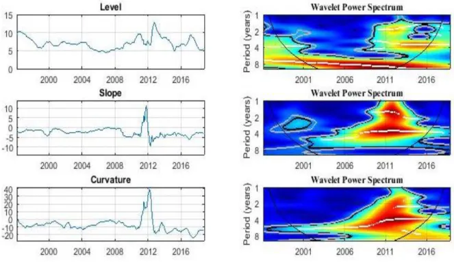
In this section, the computed yield latent factors2 and its energy measured through the variance are presented. In Figure 2, the left panels, displays the results for the three yield latent factors computed with the methodology explained in section 4.1 and in the right panel we can see the wavelet power spectrum which shows the energy of the series across time and frequency.
We can see that the long-term component always presents values higher than 5, meaning that the yield curve might have fitted well factors considering this component’s goal is to capture the long-term effects and the level factor presents higher values reflecting the price that investors demand in order to hold the sovereign bond for longer maturities.
2See appendix for the Wavelet Power Spectrum for the macroeconomic variable used in this model.
Figure 2 – Level, Slope and Curvature Estimates and its Wavelet Power Spectrum
17
Slope levels are mostly negative, by construction since a negative slope corresponds to the upward sloping yield curve exhaustively studied regarding the economic cycle. For the same reason, we can find an inverted yield in 2009 since the risk of sovereign debt crisis arose when investors had doubts if Southern European countries could roll over their debt after a devastating financial crisis which originated in the US. Yields in this context can get into a circular cycle where investors demand higher yields and higher yields bring more uncertainty about countries’ fiscal and economic abilities to accomplish the bondholder’s desires. Furthermore, the curvature latent factor shows a very similar behavior to the slope factor since it is recognized that “short-term” maturities and “medium-term” maturities’ difference is not so high as it could be due to the lack of a non-diverse list of issued bonds’ maturities.
About the Wavelet Power Spectrum3, it is simple to compare it with the previous figure since we can see very similar peaks of energy between the slope and curvature component.
For the level factor we can see that regions with higher power are located on the 8-year frequency since the beginning of the decade. Moreover, Slope’s and Curvature’s wavelet power spectrum show higher concentration of energy around the 4-year frequency starting from 2004 for both. Furthermore, there is also another ridge showing high power on the 2-year period starting from 2009, right after the financial crisis was triggered in the US with nefarious consequences for the world’s economy.
Crossing yield latent factors with macroeconomic data, we finally perform to the cross-wavelet analysis through the similarity power of the par formed by these variables.
3Blue colors correspond to temporal points across frequencies where there is an absence of power and red colors represent the areas with higher power. Levels of significance were obtained through bootstrapping with 4000 replications and are outlined as the black lines at 5% and grey lines at 10%. Maxima of undulations are located by the white stripes.
18
Wavelet coherency and phase difference are the wavelet tools used for the following analysis for the purpose to get an idea regarding changes in the dynamic relation between each par in time and frequency domains.
The visual wavelet analysis is represented in Figure 3. The visual analysis will require as a first step to set up and mark the areas where there is power among the series on the coherency graph (red areas), followed by an analysis to identify the evolution of phase difference across time, on the right side of the figure, and finally getting a conclusion by matching it with the quadrant of Figure 1. The phase difference between the two series is represented as the green line with the blue and red line representing the yield latent factor and economic activity respectively.
Regarding the level factor, we observe that except for the existence of 8-year periods there are no similar periods in which it was possible to spot a relation between level factor and activity index. Since level variations have the power to shift upwards or downwards the entire yield curve, level factors can be useful to access investors’ inflation expectations which might be a helpful tool for the central bank to apply monetary policy and get the desired effected through monetary shocks. At the 8-12 frequency band, ϕ is in the interval between π/2 and π from 2004 to 2007, suggesting that an increase in the level would anticipate a decrease in the activity index. Moreover, it might also mean a higher likelihood and considering that the time lag is close to 5, it is possible that it was a warning that a recession could arise, considering that the global financial crisis that affected the US was materialized and spread to Europe years later. This conclusion was similarly achieved by Pinho et. al (2004) who concluded, with binary models that an increase in the level leads to a higher probability of future recessions (and consequently a decrease in the activity index) in European countries such as Portugal, the UK and
19
20
Germany. Despite this conclusion, the effect seems to vanish after 2007 where these variables stop affecting each other and ϕ is near 0 implying no prediction between both time series.
Although with less significance, it is possible to spot a 5-year period during the beginning of the current century where the level factor could anticipate an increase in the macro variable since ϕ lies between 0 and -π/2.
Moving back to the next latent factor, the analysis of the slope vs activity index starts having significance in 2005, with a phase difference between 0 and π/2 for the 2-4 years band which means that an increase in the activity index will forecast an increase in the slope implying a flattened yield curve (if the slope is negative). This behavior is not in line with the usual literature in terms of causation since its main contribution relies on the ability of slope changes to predict economic recessions. At the 4-8 years band the results confirm what was previously mentioned regarding the inability of the slope to forecast the economic cycle since ϕ is near 0 until 2012 when a slightly upward curve moving the phase difference value to the interval between 0 and π/2 is observed which curiously corresponds to the turning point of the actual recession right after the speech of the ECB President Mario Draghi (casually named as “Whatever it takes”) in 2012 that had an impact on investor‘s confidence about the reliability of the Euro, with the economic growth contributing positively to the increasing of slope, leading down the short term yields against uncertainty about the inability of Portugal and other southern countries to meet with their obligations.
Despite this, most results show that the slope fails to predict the activity index for Portugal just like Hamilton (2010) stated for the US’ yield curve. The ideal would be to belong to the upper left quadrant of Figure 1 which would mean that a flattened yield curve causes a decrease in economic growth. This behavior starts in 2015 at the 4-8 band
21
but with less power since the plotted phase differences refer to the 4-8 band and the cone of influence might mislead statistical inference.
Finally, the curvature which is traditionally the less debated latent factor, does not have a long period with strong coherency with the activity index. There are periods with significant power but not within the same frequency. For instance, there is a 5-year period of significant power starting from 2000 to 2005 inside the 1~2 band period. Through phase differentiation, we see that the series is in the interval between 0 and -π/2, implying that an increase in the curvature (higher concavity) anticipates a short-run decrease of the activity index. This effect vanishes from 2005 onwards until approximately 2009 when a new effect, at levels of significance of 10%, arises in the 2~4 period band. According to the presented phase difference, similarly to previous outputs, the significant areas match with the phase difference interval between 0 and π/2. This means that an increase in the macro variable leads to an increase in the curvature (higher concavity). This effect vanishes and from 2015 onwards and the latent factor gets a new importance and its increase anticipates a decrease in the activity index. Within the 4~8 band we can interpret some results, at 10% significance levels, around 2006 where it is possible to conclude for an absence of relation between both variables.
6. Conclusion
Wavelet analysis and its tools can be very useful to fill some gaps in the literature since it extends the possibilities of studying the simultaneity between two times series regarding direction, intensity and time-lag. Wavelet tools such as phase difference and coherency provide a different approach which not only considers the time domain but also the frequency domain.
22
Crossing these two domains it is possible to get a deeper analysis when the studied variables are involved within a dynamic relation among themselves which is the case of the yield latent factors and some macroeconomic variables.
The literature exhaustively tried to exploit this relation and applied the most common methods to all possible countries when probably (and as this work project displays) there is no balanced relation between these variables. The main approach to this field should be focused in studying how to predict the relation reversal rather focusing on studying the relation between these variables as static.
Future research should focus on studying the components that alter the relation between these variables, by assessing the reasons for the existence of structural breaks in the predictability of the yield latent factors, it could be possible to control for these factors and driving them in a way to maximize the impact of monetary police through the market of sovereign bonds.
This work project used recomputed data via the Kalman filter to obtain the three latent factors based on interest rates for 5 maturities retrieved from the Bank of Portugal. The case of a more diversified basket of maturities regarding bond issuing and a longer set of data observations in the time domain would be beneficial to the literature in this field regarding the Portuguese case since there is a cone of influence within the coherency graph that at higher frequency reduces the spectrum of statistical possibilities subject to analysis.
Regarding the results it is clearly that the phase difference that showed the most values were towards the interval between 0 and π/2, suggesting that economic activity was driving the latent factors and not the other way around as most literature suggests. Despite
23
this, periods for which there was no clear relation among these variables were often detected.
7. References
[1] Aguiar-Conraria, Luís, Manuel M. F. Martins and Maria, Soares. 2012. “The yield curve and the macro-economy across time and frequencies”, Journal of Economic
Dynamics & Control, 36: 1950-1970.
[2] Aguiar-Conraria, Luís, Maria Soares, and Nuno Azevedo. 2008. “Using wavelets to decompose the time–frequency effects of monetary policy.” Physica A: Statistical
Mechanics and its Applications 387, 2863–2878.
[3] Benati, Luca, and Charles Goodhart. 2008. “Investigating time-variation in the marginal predictive power of the yield spread.” Journal of Economic Dynamics and
Control 32, 1236–1272.
[4] Chauvet, Marcelle, and Simon Potter. 2005. “Forecasting recessions using the yield curve.” Journal of Forecasting 24, 77–103.
[5] Diebold, Francis, Glenn D. Rudebusch, and Boragan Aruoba. 2006. “The macroeconomy and the yield curve: a dynamic latent factor approach.” Journal of
Econometrics 131, 309–338.
[6] Diebold, Francis, and Canlin Li. 2006. “Forecasting the term structure of government bond yields.” Journal of Econometrics 130, 337–364.
[7] Diebold, Francis, Canlin Li, and Yue Vivian. 2008. “Global yield curve dynamics and interactions: A dynamic Nelson-Siegel approach.” Journal of Econometrics, 146, 351-363.
24
[8] Estrella, Arturo, Anthony Rodrigues, and Sebastian Schich. 2003. “How stable is the predictive power of the yield curve? Evidence from Germany and the United States.” The
Review of Economics and Statistics, 85, 629–644.
[9] Estrella, Arturo, and Gikas Hardouvelis. 1991. “The term structure as a predictor of real economic activity.” The Journal of Finance 46, 555–576.
[10] Estrella, Arturo, and Frederic Mishkin. 1998. “Predicting U.S. recessions: financial variables as leading indicators.” The Review of Economics and Statistics 80, 45–61.
[11] Estrella, Arturo, and Frederic Mishkin. 1997. “The term structure of interest rates and its role in monetary policy for the European Central Bank.” European Economic
Review 41, 1375–1401.
[12] Estrella, Arturo, and Mary Trubi. 2006. “The yield curve as a leading indicator: some practical issues.” Federal Reserve Bank of New York Current Issues in Economics and
Finance 12 (5): 1–7.
[13] Evans, Charles, and David Marshall. 2007. “Economic determinants of the nominal
Treasury yield curve.” Journal of Monetary Economics 54: 1986–2003.
[14] Giacomini, Raffaela, and Barbara Rossi. 2006. “How stable is the forecasting performance of the yield curve for output growth?” Oxford Bulletin of Economics and
Statistics 68: 783–795.
[15] Goupillaud, Pierre., Alex Grossman, and Jean Morlet. 1984. “Cycle-Octave and Related Transforms in Seismic Signal Analysis.” Geoexploration 23, 85–102.
[16] Hamilton, James D. 2010. “Calling recessions in real time.” International Journal of
25
[17] Harvey, Campbell. 1988. “The real term structure and consumption growth.” Journal
of Financial Economics 22, 305–333.
[18] Haubrich, Joseph.G., and Ann M. Dombrosky. 1996. “Predicting real growth using the yield curve.” Federal Reserve Bank of Cleveland Economic Review 32, 26–34.
[19] Jorion, Philippe, and Frederic Mishkin. 1991. “A multicountry comparison of term-structure forecasts at long horizons.” Journal of Financial Economics 29, 59–80.
[20] Mishkin, Frederic. 1990. “What does the term structure tell us about future inflation?” Journal of Monetary Economics 25, 77–95.
[21] Nelson, Charles, and Andrew F. Siegel. 1987. “Parsimonious modelling of yield curve.” Journal of Business 60, 473–489.
[22] Rua, António. 2004. “A new coincident indicator for the Portuguese economy.”
Economic Bulletin and Financial Stability Report Articles.
[23] Pinho, Carlos, Mara Madaleno, Isabel Maldonado, and Francisco Rodríguez de Prado. 2014. “Predictive power of the term structure of interest rates over recessions in Europe.” 8th Annual Meeting of the Portuguese Economic Journal.
[24] Wright, Jonathan H. 2007, “The Yield Curve and Predicting Recessions.” Finance
and Economics Discussion Series Divisions of Research & Statistics and Monetary Affairs Federal Reserve Board.
[25] Bank of Portugal. 2018. “Yield on fixed rate treasury bonds”. Retrieved from BPstat. [26] Bank of Portugal. 2018. “Economic Activity Coincident Indicator”. Retrieved from BPstat.
26