The nugget-effect approaches of SAKWeb
©for
environmental modelling
J. Negreiros, M. Painho, A. C. Costa, P. Cabral & T. Oliveira
Instituto Superior de Estatística e Gestão de Informação, Universidade Nova de Lisboa, Lisboa, Portugal
Abstract
Ordinary Kriging (OK) seems to achieve better spatial interpolation results than other methods regarding environmental pollution, for instance, although sampling distribution can turn out to be a problem. This latter issue leads to a crucial topic identified as the nugget-effect, the distance interval in which capturing spatial dependency is most important. SAKWeb© developments have been made using four approaches to this factor: (1) with and (2) without nugget-effect, (3) micro-scale component and (4) measurement error inclusion that leads to a non-exact Kriging version. Although no spatial patterns can be found regarding which nugget-effect fits best, the possibility of simulating different on-the-fly models and comparing discrepancy among them is already significant in a W3 context.
Keywords: GIS, geocomputation, environmental modelling, Kriging, measurement error, nugget-effect.
1 Introduction
For many expertise’s such as Longley et al. [8], spatial environmental analysis within GIS has nothing to do with the general ability to describe spatial data, generally incorporated in all commercial GIS but it presents the challenge, given a spatial pattern, to explore it with an appropriate model and represent it with a graphical display. Certainly, to describe is not to explore. As Murteira [9] confirms, exploring is a detective work, a search for clues and evidence, while describing is a job of judgment, a job of analyzing and evaluating clues.
Nevertheless, GIS and spatial analysis has been touched by the major aftermath of the last century: Internet. In effect, users now have the ability to
collect and to explore large amount of geo-referenced data. With the advent of Web technology and modern wireless computing, it becomes necessary to develop WWW software for geo-environment interpolation to understand the often-complex spatial autocorrelation that exist among the samples collected in space. The Internet geostatistical solution and, particularly, the close linkage of spatial autocorrelation, Kriging and uncertainty measures become, therefore, some major components for SAKWeb©.
“SAKWeb© is the first free Web software in operation that provides access to a wider audience” (Negreiros [10], Negreiros and Painho [11], Negreiros et
al [12]). It is not a comprehensive statistical package in the traditional way for
solving everyone’s problems. Written for an IIS® Web service with ASPs®, Javascript, WebChart® and Flash®, “it was developed with the philosophy that spatial autocorrelation and Kriging software is needed as a learning tool by individuals with limited geostatistical knowledge” (Negreiros and Painho [13, 14]). Yet, it can also satisfy the needs of individuals with more training. SAKWeb© deals with Kriging interpolation in conjunction with spatial association measures in a Web continuum process instead of a loose local spatial function. From this view point, an element of its originality and innovation can, thus, be appreciated.
In this article, one key topic will be discussed: It is quite common to have a discontinuity at the variogram origin although major Kriging software forces it to be zero at zero distance. With SAKWeb©, four nugget-effect combinations are depicted in order to add some software value to this dilemma.
2 The nugget-effect dilemmas
When no nugget-effect, γ(0), is introduced or when the phenomenon is well structure such as ambient ozone interpolation with a quadratic model near the origin, negative weights are more likely. The screen-effect and clustered points are also likely to produce negative weights and, thus, the possibility to estimate beyond the available sample extremes become real and negative concentrations can be achieved, the non-convexity property. This also includes an increase in the mean squared prediction error.
The discontinuity of the variogram origin should not occur in most spatial environmental processes because space is continuous most of the time, although particular Earth processes such as gold mineralization do not respect this pattern. Nevertheless, the variogram should be continuous at the origin. “Remember that one of our basic assumptions is physical continuity of the phenomena being measured” (Clark and Harper [3]). Furthermore, “a free version of the measurement error should be predicted because when predicting at a particular location, the investigator wants to know what actually exists at that location and not the value distorted by, for example, laboratory measurement error” (Cressie [4]).
Existing software considers the nugget-effect zero, γ(0)=0, although the variogram does not tend towards zero as the lag distance approaches zero, therefore, leading to a sharp rise for very small distances. Yet, Kriging becomes
an exact estimator reflected in a strange looking map due to a sudden jump in the predicted collected samples. According to Clark and Harper [3], if the nugget-effect is treated as an intercept with the variogram axis so that γ(0)=C0, two samples taken at the same location could have a variance of 2C0. Thus, another possibility to handle this factor is to consider γ(0)=C0 while 2C0 must be added to the final Kriging variance.
For Atkinson [2], if the source of measurement error is external, e.g., the mechanical noise, removing it is to subtract from the initial variogram some value from all lags. If the source of measurement error is internal, e.g., site position error, removing it is to subtract some function type that decreases from the variogram value at lag of zero to zero at some positive lag. In extreme cases, if the variogram is a pure nugget-effect or the variogram range is less than the distance between samples, the best estimation would be the sample arithmetic average because adjacent points are uncorrelated. With regard to major circumstances, the shift of massive weights towards the closest sample becomes a reality, including the tendency of the LaGrange multiplier factor towards negative values. Certainly, the nugget-effect is of critical importance in spatial estimation.
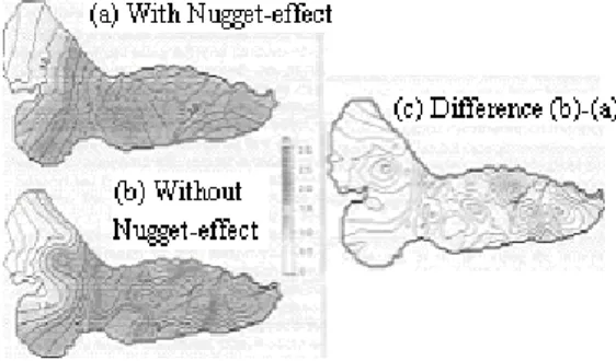
As reported by Hock and Jensen [6] in their valley research in Sweden, the Kriging interpolation of glacier mass reveals a considerable difference with respect to the spatial distribution up to 0.66m. It is clearly a wide estimate range without the nugget-effect (see figure 1). For Isaaks and Srivastava [7], particular differences in the nugget-effect at different thresholds will cause IK with different variogram models at different cutoffs to produce results that are quite different from those produced by median IK.
Figure 1: The OK interpolation of a Swedish glacier mass with and without the nugget-effect.
Unless some additional close samples are available, geostatisticians must guess the variogram shape near the origin, especially when the distance from the point being estimated to a particular sample is small. For Armstrong [1], the nugget-effect and the origin slope are the most important features for fitting the variogram. With well-structured variograms, most weights are concentrated in locations around the estimated one. With poor situations, Kriging improves as the range increases or more samples are added, leading to a smoother variogram.
A rough rule of thumb is that eight samples are included when the nugget is near zero, increasing to twenty when it is more than 50% of the sill.
3 SAKWeb
©strategies
Because of transition models depends on the variogram behavior near the origin, SAKWeb© presents four strategies for the nugget-effect. The default is to consider that observations are precise and accurate, although sudden jumps at the variogram origin may emerge. This means forcing the nugget-effect to zero at zero distance: γ(0) = 0; γ(h) = Spherical, Exponential and Gaussian model, if 0<h<=range; γ(h) = sill = C0 (nugget-effect)+C1(partial sill), if h>range.
Another possibility is to consider γ(0)=0 in a continuous mode. Two extra approaches are also depicted: the first regards the micro-scale component and the second includes the measurement error.
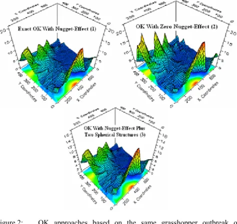
With the micro-scale component method, the nugget-effect is divided into two factors: γ1(0<=h<=shortest sampling interval)=Spherical, Exponential and Gaussian first model; γ2(shortest sampling interval<h<=range)=Spherical, Exponential and Gaussian second model. The first micro-scale range equals the shortest sampling interval (SSI) lag, its nugget-effect is zero while its total sill matches the extrapolated value of the second variogram structure, that is, the given value of the second variogram structure at SSI distance is the first variogram sill parameter. For Cressie [4], this vision reflects different processes of variability on different scales: Z(s)=µ(s)+W(s)+η(s)+ε(s) where µ(s) is the large-scale deterministic variation, W(s) is the smooth small-scale variation (the intrinsically stationary process whose variogram range exists and is larger than min{||si-sj||}), η(s) is the microscale variation whose variogram range exists and is smaller than min{||si-sj||}) and ε(s) is a zero-mean white-noise process, independent of W and η. As Soares [17] demonstrated, the sums of basic correlation structures are often used to model multiple ranges in nested models. This happens because the sum of known positive definite models is also a positive definite one, leading, thus, to great flexibility in modeling variograms. This methodology will also lead to an already significant feature of SAKWeb© and testified by an independent survey to 20 respondents in January 2003: The possibility of simulating different on-the-fly models and comparing discrepancy among them. Most users really appreciate this capability to generate several Kriging surfaces automatically and compare them without any extra work (see figure 2).
If measurement error, Cme, is given, the fourth approach, the measurement error factor is included within the covariances matrix between the estimation and the samples, γB(x0,xi). In this case, this Kriging B matrix is the same unless it coincides with the samples locations, a non-exact version of the interpolator. Therefore, the measurement error must be setup (instead of zero of the exact version) and a smoother prediction of the Kriging estimations thus becomes real for the available samples. Since the Ordinary Kriging estimations are the same whether the measurement error is considered or not, this is the main cause of the SAKWeb© choice: Instead of the final OK map being laid out, only the available samples are estimated (see figure 3). This factor must also be subtracted from the
variance prediction error, leading to a lower standard error surface: 2 2 OK i 0 i me i 0 i me σ =
∑
w γ(x ,x )+Ψ-c =σ -∑
w C(x ,x )-Ψ-c , where w i is OK weight, 0 iγ(x ,x ) equals the variogram value between the estimated point and the sample, Cme represents the measurement error, σ2 signifies sample variance, C(x , x )0 i stands for the covariance between the estimated point and the sample and is the LaGrange parameter.
Figure 2: OK approaches based on the same grasshopper outbreak of Colorado (1993).
Figure 3: OK between the exact version and the one with measurement error.
It is crucial to emphasize that the prediction standard error of the samples is zero when no measurement is considered, a situation not contemplated when the
measurement error is included, for instance, due to last night’s rainfall. As stated by Cressie [4], “it is important to include measurement error, which is often the case, within the Kriging system”.
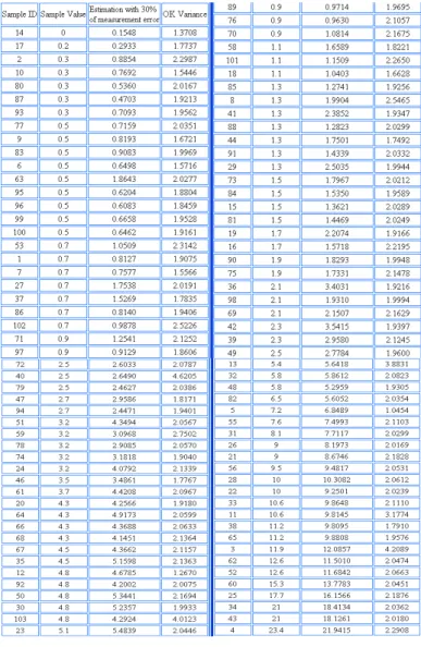
In terms of internal computation, suppose that the user has five samples (x coordinate, y coordinate, sample value) regarding a heavy-metal contaminated soil: (1,5,100), (3,4,105), (1,3,105), (4,5,100) and (5,1,115). His goal is to estimate the (1,4) unsample location with OK, where the linear variogram equals γ(h)=2+13.5×distance. The A-1, B and W matrices are as Figure 4 shows.
A-1= 0 32.19 29 42.5 78.37 1 = -0.02392 0.006659 0.013706 0.006126 -0.00257 0.329226 32.19 0 32.19 21.19 50.67 1 0.006659 -0.04069 0.009486 0.019637 0.004903 -0.18427 29 32.19 0 50.67 62.37 1 0.013706 0.009486 -0.02445 -0.00358 0.004838 0.176614 42.5 21.19 50.67 0 57.66 1 0.006126 0.019637 -0.00358 -0.02633 0.004141 0.265995 78.37 50.67 62.37 57.66 0 1 -0.00257 0.004903 0.004838 0.004141 -0.01131 0.412432 1 1 1 1 1 0 0.329226 -0.18427 0.176614 0.265995 0.412432 -42.8173 B= 15.5 W= 0.459169877 OK Estimation= 102.8902 sample1 100 29 0.104453911 sample2 105 15.5 0.461557935 sample3 105 44.69 -0.01380446 sample4 100 69.5 -0.01137726 sample5 115 1 0.230774028
Figure 4: The OK system of the working example.
A-1= 0 32.19 29 42.5 78.37 1 = -0.02392 0.006659 0.013706 0.006126 -0.00257 0.329226 32.19 0 32.19 21.19 50.67 1 0.006659 -0.04069 0.009486 0.019637 0.004903 -0.18427 29 32.19 0 50.67 62.37 1 0.013706 0.009486 -0.02445 -0.00358 0.004838 0.176614 42.5 21.19 50.67 0 57.66 1 0.006126 0.019637 -0.00358 -0.02633 0.004141 0.265995 78.37 50.67 62.37 57.66 0 1 -0.00257 0.004903 0.004838 0.004141 -0.01131 0.412432 1 1 1 1 1 0 0.329226 -0.18427 0.176614 0.265995 0.412432 -42.8173 B= 0 W= 0.999985816 OK Estimation= 100.000 sample1 100 32.187 0.000113306 sample2 105 29 -4.1178E-05 sample3 105 42.5 -7.0745E-05 sample4 100
78.368 1.28018E-05 No measurement error sample5 115 1 -0.00044976 A-1= 0 32.19 29 42.5 78.37 1 = -0.02392 0.006659 0.013706 0.006126 -0.00257 0.329226 32.19 0 32.19 21.19 50.67 1 0.006659 -0.04069 0.009486 0.019637 0.004903 -0.18427 29 32.19 0 50.67 62.37 1 0.013706 0.009486 -0.02445 -0.00358 0.004838 0.176614 42.5 21.19 50.67 0 57.66 1 0.006126 0.019637 -0.00358 -0.02633 0.004141 0.265995 78.37 50.67 62.37 57.66 0 1 -0.00257 0.004903 0.004838 0.004141 -0.01131 0.412432 1 1 1 1 1 0 0.329226 -0.18427 0.176614 0.265995 0.412432 -42.8173 B= 0.6 W= 0.985632768 OK Estimation= 100.236 sample1 100 32.187 0.004107719 sample2 105 29 0.008185204 sample3 105 42.5 0.003608176 sample4 100 78.368 -0.00153387 sample5 115 1 0.197263267
With Measurement Error
Figure 5: The OK estimation considering with and without measurement error.
The final prediction equals 102.8202 with a LaGrange factor of 0.2307. Since no samples have a zero distance from the interpolation site, the OK with measurement error does not have any impact on the A and B matrices. However,
if the estimated site becomes the first sample, then both OK versions yield different results. Considering a 30% measurement error of the nugget-effect (γ(0)=0.3×(2+13,5×0)=0.6), for instance, the B matrix and the final estimate becomes different, as Figure 5 shows.
Note that the final interpolation of the exact version computes the sample itself, a situation not followed by the non-exact version (the variance becomes 0.5913). Further, the OK variance of the case above is reduced from 16.1235 to 15.5235, a generic situation confirmed by SAKWeb© with the 1993 grasshopper dataset of Colorado, an environmental monitoring issue (see Figure 6).
Figure 6: Comparison between the exact version of SAKWeb© OK and the one with 30% measurement error.
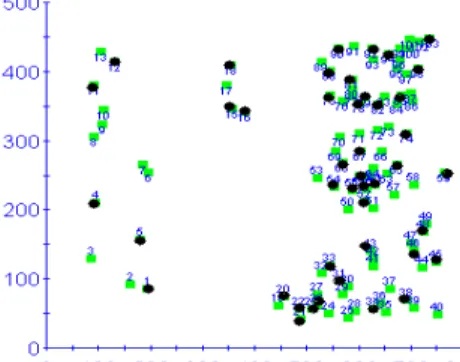
It is clear that the measurement error of 30% has an impact on the OK: 58% of the estimates are higher than the original samples and, therefore, 42% are lower. According to Figure 7, no spatial patterns can be found for the measurement error effect for middle values but lower samples leads to higher estimations and vice-versa: The sites with grasshopper infestation of less than 1.1 (thirty sites) gives higher OK estimates; The twenty-one samples that register densities higher than 5.8 produce lower estimations; Of the fifty-one observations whose values vary between 1.1 and 5.8, 55% have lower densities than the OK estimates.
Figure 7: The spatial location of the grasshopper, Colorado, densities where the dark dots represent the sites whose OK estimates with a 30% measurement error are lower than the original samples.
4 Conclusions
The current e-Learning trend illustrates a strong development in the distribution of brain-ware know-how, supported by the time and cost savings of the Web infrastructure. “Also, statistical comparisons between traditional and distance learning reveal no major differences in terms of student success and failure” (Negreiros [10], Negreiros and Painho [11]). Although some companies still show resistance to recruiting employees that had this type of education, the fact is that the opinions of business executives are shifting and accepting this new culture. In conjunction with the need to share educational contents of spatial analysis, SAKWeb© follows this trend by giving access to hypermedia resources and creating new software features, particularly when compared with the traditional approaches: GIS modules, statistical tools or independent software. One of those characteristics is discussed here.
The discontinuity of the variogram origin can be viewed as a nonsense situation since landscape realities or natural hazards are considered a continuous surface. Among all variogram factors, the nugget-effect is also the most unpredictable because of the lack of close samples. So, SAKWeb© offers four strategies to handle the nugget-effect: γ(0) = 0; γ(0) = 0 but including C0 for superior lags; γ(0) with micro-scale, γ1(h), and long-range, γ2(h), assessment;
If measurement error is given, this attribute will be incorporated within the Kriging system. The capability to compare on-the-fly models among them is a further possibility.
At last, it is critical to emphasize that self-inferences of data choice, weight assignment and geographical knowledge, inclusion of soft information, procedure selection and previous user experience are central factors in guiding the process of spatial analysis. For instance, “the long-range nickel variogram structure for the Jura region in Switzerland is closely related to the control asserted by the rock type, while the short-range one for cadmium suggests the local impact of man-made contamination” (Goovaerts [5]). Kriging does not consist of throwing spatial data into a black-box response program. The secret is some kind of mix and match strategy in which both the analysis machine and the analyst concentrate on doing what each is best at. “The effectiveness of spatial analysis requires an intelligent user, not just a powerful computer” (Longley et
al. [8]). Although Costumer-Of-The-Shelf solutions are regarded as a full
black-box, this should be interpreted from the viewpoint of computer knowledge because geostatisticians should not be concerned about input-output data flows, intermediate calculus, the choice of programming language or other technical matters.
References
[1] Armstrong, M., 1998, Basic Linear Geostatistics, Springer, 154 p.
[2] Atkinson, P., 1997, A Method for Describing Quantitatively the Information, Redundancy and Error in Digital Spatial Data, in Innovations in GIS 3, Taylor & Francis, p. 85–96.
[3] Clark, I., Harper, W., 2000, Practical Geostatistics 2000, Ecosse North America, Chapter 9 (CD-ROM).
[4] Cressie, N, 1993, Statistics for Spatial Data, John Wiley & Sons, New York, 887 p.
[5] Goovaerts, P., 1998, Geostatistics in Soil Science: State-Of-The-Art and Perspectives, Geoderma, 89.
[6] Hock, R., Jensen, H., 1999, Application of Kriging Interpolation for Glacier Mass Balance Computations, in Geografiska Annaler, 81, p. 611–619. [7] Isaaks, E., Srivastava, R., 1989, An Introduction to Applied Geostatistics,
Oxford University Press, New York, 551 p.
[8] Longley, P., Goodchild, M., Maguire, D., Rhind, D., 2001, Geographical Information Systems and Science, John Wiley & Sons, 454 p.
[9] Murteira, B., 1993, Análise Exploratória dos Dados – Estatistica Descritiva, McGraw Hill de Portugal, 329 p.
[10] Negreiros, J., 2004, SAKWeb (Spatial Autocorrelation and Kriging Web) – A W3 Computation Perspective, Unpublished Ph.D. Thesis, 449 p.
[11] Negreiros, J., Painho, M., 2005, The Web Platform for Spatial Statistical Analysis (#92), The Portuguese Conference of Information Systems 05, ISBN 13:978-972-789-219-8, Bragança, Portugal.
[12] Negreiros, J., Costa, A., Painho, M., Lopes, I., 2006, :Spatial Autocorrelation and Association Measures, Encyclopedia of Networked and Virtual Organizations, Idea Group Reference.
[13] Negreiros, J., Painho, M., 2006, SAKWeb© – Spatial Autocorrelation and Kriging Web Service, Geo-Environment & Landscape Evolution II, WIT Press, p79-89, ISBN 1-84564-168-X, Rhodes, Greece.
[14] Negreiros, J., Painho, M., 2006, SAKWeb© – Spatial Autocorrelation and Kriging Web Service (Part II), Internet Research 7.0: Internet Convergences (http://paginas.ulusofona.pt/p2203), Brisbane, Australia (Sep 06)
[15] Negreiros, J., Costa, A., Painho, M., Santos, J., 2007, Autocorrelation, Autoregression and Kriging: The Spatial Interpolation Issue, International Statistic Institute 56th Conference, Lisboa, Portugal.
[16] Negreiros, J., Costa, A., Painho, M., Santos, J., Lopes, I., 2007, Geostatistical Analysis: Software Flashpoint, Geocomputation 2007, Dublin, Ireland.
[17] Soares, A., 2000, Geoestatistica para as Ciências da Terra e do Ambiente, IST Press, 206 p.