A Work Project, presented as part of the requirements for the Award of an
International Masters in Finance from the
NOVA – School of Business and Economics
and a
Professional Master in Finance from the
Fundação Getúlio Vargas – São Paulo School of Economics
Macroeconomic Indicators and Systematic Risk - Is there a difference
between Emerging and Developed Markets?
Hubertus Tassilo Schlögl
Nova SBE Student Number: 3371 & 29373
FGV-EESP Student Number: 338933
A project carried out on the Double Degree EESP-FGV,
under the supervision of:
Professor Martijn Boons (Nova SBE, Lisbon, Portugal)
Professor Joelson Sampaio (EESP-FGV, São Paulo, Brazil)
Date:
3
rdJanuary 2018
2
Macroeconomic Indicators and Systematic Risk - Is there a difference
between Emerging and Developed Markets?
Abstract:
This explorative study is about the influencing effects of US macroeconomic announcements on changes in systematic risk with the focus on the difference between emerging and developed markets. Seven different US macroeconomic indicators have been examined and used to estimate betas as a proxy for the systematic risk around the announcement dates. In the period from 1996 until 2017, betas have been estimated over a three-month pre- and post window, resulting in 27 announcements per US macroeconomic indicator. The study also tries to provide insights of the consequences for portfolio managers, based on patterns of changes in betas and their relationship with changes in Sharpe ratios. The study results reveal that betas change consistently over the sample period, however, to a small magnitude. Also, the changes in mean Sharpe ratios around these announcement dates have not been found as statistical significant. However, the study results indicate that there is a positive relationship between changes in Sharpe ratios and changes in betas for developed countries as the Pearson correlation coefficient illustrates.
3
Table of Contents
1) Introduction ... 5
2) Literature ... 7
2.1) Systematic Risk and its Determinants ...7
2.1.1) Systematic Risk and the Micro Environment ...8
2.1.2) Systematic Risk and Mergers & Acquisitions ...10
2.1.3) Systematic Risk and the Macro Environment ...10
2.2) Macroeconomic Indicators ...11
2.2.1) Interest Rates ...12
2.2.2) Trade Balance ...13
2.2.3) Business Inventories ...14
2.2.4) Consumer Price Index ...15
2.2.5) Unemployment Rates ...16
2.2.6) Nonfarm Payrolls ...17
2.2.7) University of Michigan Consumer Sentiment Index ...18
3) Methodology & Data ... 19
3.1) Methodology ...19
3.2) Data ...23
4) Results ... 24
4.1) Results Pooled Sample ...24
4.1.1) Interest Rates ...24
4.1.2) Trade Balance ...25
4.1.3) Business Inventories ...26
4.1.4) Consumer Price Index ...26
4.1.5) Unemployment Rates ...27
4.1.6) University of Michigan Consumer Sentiment Index ...28
4.1.7) Nonfarm Payrolls ...28
4.2) Results Emerging Markets ...29
4.2.1) Interest Rates ...29
4.2.2) Trade Balance ...29
4.2.3) Business Inventories ...30
4.2.4) Consumer Price Index ...31
4.2.5) Unemployment Rates ...31
4.2.6) University of Michigan Consumer Sentiment Index ...32
4.2.7) Nonfarm Payrolls ...32
4
4.3.1) Interest Rates ...33
4.3.2) Trade Balance ...34
4.3.3) Business Inventories ...34
4.3.4) Consumer Price Index ...35
4.3.5) Unemployment Rates ...35
4.3.6) University of Michigan Consumer Sentiment Index ...36
4.3.7) Nonfarm Payrolls ...36
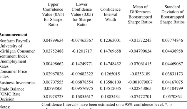
4.4) Results Bootstrap Confidence Intervals ...37
4.4.1) Results Bootstrap Confidence Intervals Pooled Markets Portfolio ...38
4.4.2) Results Bootstrap Confidence Intervals Emerging Markets Portfolio ...40
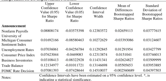
4.4.3) Results Bootstrap Confidence Intervals Developed Markets Portfolio ...43
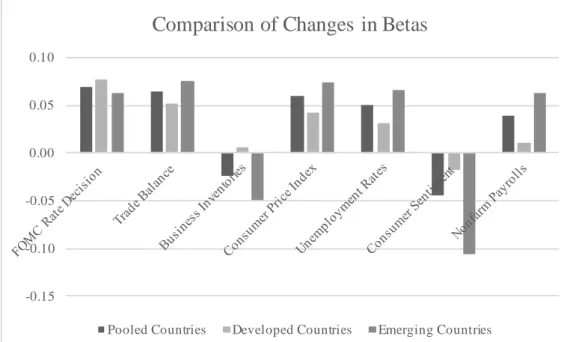
4.5) Patterns of Changes in Betas among Emerging and Developed Markets ...45
4.6) Relationship between Sharpe Ratios and Changes in Betas ...51
4.7) Implications for Portfolio Managers ...54
5) Conclusion ... 54
6) Limitations & Further Research ... 56
7) References ... 57
5
1. Introduction
Within finance, risk and return always have been a major subject of study. Many practitioners make use of different kind of back testing procedures to find patterns in stock prices and risks, to build profitable investment strategies upon them. Hence risk and return are an inseparable combination. This fundamental leads to the tradeoff that higher return comes at the expense of higher risk. According to the finance literature, risk is segregated into two components: ‘systematic’ and ‘unsystematic risk’ (Robichek & Cohn, 1974). While idiosyncratic risk can be diversified away, systematic risk cannot. Furthermore, the literature reveals that the beta coefficient is the most commonly used coefficient to represent systematic risk of a stock with respect to its benchmark or the market portfolio. Beta is estimated by taking the covariance of a stock and its market portfolio over the variance of the market portfolio. Consequently, high beta stocks ( 1) have a higher risk than the market but also might have higher returns. Even though, beta has been studied quite intensively over the past decades, there is still only a little evidence to what degree betas response to changes in the economic environment. The work from Robichek & Cohn (1974) and Andersen, Bollerslev, Diebold & Wu (2005) had revealed that systematic risk is indeed influenced by macroeconomic variables and that it is time varying. Robichek & Cohn (1974) could provide significant findings for the two macroeconomic variables of GDP and inflation. However, the authors could only provide insights on these two macroeconomic indicators. Therefore, this study tries to build on their findings and to provide new insights, whether the actual announcements of such macroeconomic variables have any effects on betas. Furthermore, the literature does not reveal if there is a difference between emerging and developed economies with respect to the effect of macroeconomic news on betas. Out of this, this study tries to contribute to this gap in the literature by answering the following research question: ‘To what extent does changes in systematic risk differ between developed
6
motivation, why it seems to be reasonable to examine the effect of macroeconomic announcements on systematic risk, is based on the fact that stock market prices are supposed to reflect companies’ fundamentals. Since these fundamentals depend on the expected present value of future dividend payouts and in turn those dividend payouts must reflect the real economic environment, mainly measured by industrial production and gross domestic product GDP (Shapiro ,1988), the assumption that macroeconomic events also drive betas seem to be acceptable. In total, this study examines the announcements of Unemployment rates, Trade Balance, Consumer Price Index, Interest rates, Business Inventories, Nonfarm Payrolls, and the University of Michigan Consumer Sentiment Index. The reason for the selection for most of these macroeconomic indicators is based on the findings from Flannery & Protopapadakis (2002), who have identified CPI, PPI, Monetary Aggregates, Employment Report, Balance of Trade, and Housing Starts as strong candidates for risk factors. Their reasoning for considering these factors as risky is based on the assumption that announcements regarding these factors are either affecting returns or increasing the market’s conditional volatility. The study’s aim is based on the same fundament. Preliminary results of this paper indicate that betas are indeed changing in response to macroeconomic announcements, while changes in Sharpe ratios of emerging and developed market portfolios seem not to be affected by these announcements. Within the first part of this study, the existing literature regarding systematic risk and macroeconomic indicators will be reviewed. The second part will explain the methodology and data used to analyze the effect of macroeconomic announcements on systematic risk and how this study tries to relate it to implications for portfolio managers. Finally, within the third and last part of the study, the results and conclusions will be drawn.
7
2. Literature
Before describing the analysis, prior findings within the finance and economic literature regarding determinants of betas and the importance of macroeconomic indicators will be emphasized.
The analysis of announcements within the world of finance almost knows no limits. With the most famous and popular ‘Event Study’ methodology, introduced by Fama et al. (1969), the analysis of events and in particular the analysis of announcements on equities, fixed income but also on merger & acquisition activities among others, have been further and further developed. The importance of announcements on financial markets has also been confirmed by practitioners, when Goldberg & Leonard (2003) were analyzing the effects on economic news on international bond markets on behalf of the Federal Reserve Bank in New York. According to the authors, economic announcements are an important source of information, affecting global yields. In particular, the authors found that the largest yield moves have been associated with announcements on Unemployment rates, real GDP growth, and Consumer Sentiment. As one can clearly observe, the importance of economic announcements is undisputable. However, before presenting the analysis regarding announcements on macroeconomic indicators, it is crucial to determine which announcements might have the strongest effects on betas. In order to do this, prior literature findings regarding betas and therefore systematic risk will be reviewed to see how betas are behaving within financial and economic analyses.
2.1 Systematic Risk and its Determinants
One of the most common concepts within the finance literature was the emergence of the Capital Asset Pricing Model (CAPM). The CAPM, developed by William Sharpe, Jack Treynor, John Lintner and Jan Mossin in the early 1960s relates the price of an asset to the risk-free rate, prevailing in a country and to the market premium.
8
In the case of the CAPM, the beta coefficient is estimated by dividing the covariance between the asset and the market index by the variance of the market, representing the systematic risk. With the emergence of the CAPM as an extension to Markowitz portfolio theory from 1952, the foundation was laid for incorporating the systematic risk for price discoveries for equities and portfolio analyses.
2.1.1 Systematic Risk and the Micro Environment
Most of the finance literature regarding systematic risk has been conducted on a micro level. The literature has revealed that operating efficiency, measured by asset turnover ratios, has a negative relationship to the systematic risk of companies. According to Logue & Merville (1972), a higher operating efficiency leads to higher profits of companies and thus have a lower probability of default, which in turn reduces the systematic risk for shareholders. These findings have been confirmed by Gu & Kim (1998), who examined the effect of asset turnover ratios on systematic risk for 35 casino firms in the United States throughout the 90s. The authors have revealed that rather than expanding the casino’s operations, higher operational efficiencies (higher asset turnover ratios) resulted in lower systematic risk.
Furthermore, a company’s liquidity seems to play an important role for systematic risk as well. According to Logue & Merville (1972) there is a negative relationship between liquidity and systematic risk. The authors explain this relationship with the fact that high liquidity indicates low level of short – term liabilities, which lower systematic risk. These findings have been confirmed by Moyer & Chatfield (1983) later within the literature.
However, also contrary findings regarding the relationship between systematic risk and liquidity have been published. According to Jensen (1984), systematic risk is also increased (decreased) with a higher (lower) level of liquidity. The author is explaining this phenomenon with the agency theory, as high liquidity rises the firm’s agency cost of free cash flow and hence
9
its systematic risk. Similar findings have been revealed earlier by Beaver & Manegold (1975), who found a negative relationship between firm’s current ratios and systematic risk. However, a greater proportion of the literature’s findings indicate a positive relationship between liquidity and systematic risk (Pettit & Westerfield, 1972, Rosenberg & McKibben, 1973 and Borde ,1998). According to these authors, there is a positive relationship between liquidity ratios and systematic risk.
Next, profitability has been found to have a negative relationship with systematic risk. According to Logue & Merville (1972), higher profitability of a firm reduces the probability of default and hence reduces the systematic risk for shareholders. These findings are confirmed by Scherrer & Mathison (1996), who analyzed the systematic risk for REITs, by revealing that the stability of the operational cash flow indicates that the property is being managed profitable, which in turn reduces the systematic risk.
Furthermore, there are also many studies about the effect of leverage on firm’s systematic risk. After the introduction of the Modigliani and Miller (MM) propositions in the 1950s, several studies have been conducted to analyze a firm’s systematic risk related to its capital structure. According to Hamada (1972), systematic risk is increased whenever a firm is increasing its leverage while maintaining a fixed level of equity. With the mean – standard deviation of the CAPM, the covariance of an asset’s return with the return of the market portfolio is greater for a stock with a higher debt – equity ratio than for a firm with a lower debt – equity ratio. Assuming the MM propositions are correct, roughly 21% to 24% of a firm’s systematic risk can be explained by adding leverage to the firm’s capital structure. These findings have been complemented later within the finance literature, when Mandelker & Rhee (1984) were analyzing the degree of operating leverage (DOL) and the degree of financial leverage (DFL) on a firm’s systematic risk. The authors revealed that the DOL and DFL are magnifying the variation in beta of a company. In other words, systematic risk is not only increased by financial
10
leverage but also by operational leverage. Similar findings regarding the positive relationship between leverage and systematic risk have been published later within the literature. According to Moyer & Chatfield (1983), Amit & Livnat (1988), and Kim, Gu & Mattila (2002), there is a positive relationship between systematic risk and a firm’s leverage. The authors describe their findings with the fact that a higher debt leverage exposes their shareholders to a higher systematic risk. Even though, the literature agrees upon a positive relationship between a firm’s greater reliance on leverage and higher systematic risk for shareholders, this relationship has been found as not linear (Melicher, 1974).
2.1.2 Systematic Risk and Mergers & Acquisitions
Another area of the analyses of systematic risk within the finance literature is the effect of merger and acquisition activities on changes in systematic risk. According to Chatterjee & Lubatkin (1990), systematic risk of bidding firms within a M&A process can reduce their systematic variability in the returns of their securities by acquiring or merging with target companies which complement through their non – competing products. Furthermore, the literature revealed that systematic risk can be reduced, when growing through merger and acquisitions activities when lower portions of debt financing are used (Kim, Gu & Mattila, 2002).
2.1.3 Systematic Risk and the Macro Environment
As already mentioned empirical findings regarding systematic risk and the economic environment are mainly focused on the micro level. Mainly the relationship between beta and liquidity, leverage, operational efficiency, profitability, dividend payout, firm size and growth have been analyzed. However, to what extent systematic risk is influenced by macroeconomic indicators is less elaborated. There is still some evidence that the economic environment is determining a company’s beta and therefore its systematic risk. Robichek & Cohn (1974), who
11
were testing the principal hypothesis, indicate that the systematic riskiness of the common shares of companies are related to the economic conditions. The authors revealed that a small but statistically significant number of companies’ systematic risk varied due to GDP and inflation, by comparing estimated betas in times with high economic growth and inflation versus low economic growth and inflation. Even if Robichek & Cohn (1974) could not give any explanations why the systematic risk changed due to macroeconomic events, the authors justified their assumption that even if the systematic risk is not changing because of macroeconomic indicators, it is difficult to expect that it would remain the same.
2.2 Macroeconomic Indicators
The elaboration of the literature’s most frequently cited macroeconomic indicators is used as the basis for the selection of the study’s U.S. macroeconomic announcements. Since there is no exact comparable study within the literature regarding the analysis of macroeconomic announcements on betas, a starting point had to be set when selecting macroeconomic indicators. The literature has been screened mainly on macroeconomic indicators that are most influential on financial markets and especially on equity and bond markets. The literature’s landscape regarding macroeconomic announcements focuses on two distinct categories: the influence and creation of abnormal returns and the influence on volatilities around announcement dates. Since the main input of systematic risk or beta is the covariance and variance of the stock and its market return, it seems to be reasonable to focus and follow the most frequent cited macroeconomic determinants of equity prices and volatilities. In addition, information regarding bond markets seem to be acceptable as well, due to the basic relationship between interest rates and bond and equity markets, respectively.
According to the literature, the most influential and frequently examined and cited macroeconomic indicators for financial markets are: Interest rates, Unemployment rates,
12
Inflation, Exchange rates, Imports, Exports, and Trade Balance. However, to what extent these indicators are influencing financial markets depend on several factors such as economic development of a country, whether it is a long term or short term analysis and so forth. This study will review prior findings about Interest rates, Trade Balance, Business Inventories, Consumer Price Index, Unemployment rates, Nonfarm Payrolls, and findings regarding the University of Michigan Consumer Sentiment Index. Even though, the last two indicators are less examined within the finance literature, this study will include them to also add new insights about those two indicators.
Before reviewing prior results of the literature, possible asymmetrical findings of macroeconomic variables on stock returns could be explained twofold, with asset prices reacting to volatility feedback (Campbell & Hentschel, 1992) and because asset prices tend to react to behavioral aspects of risk assessment such as the prospect theory (Patel et al., 1991).
2.2.1 Interest Rates
To begin with one of the most influential indicators, Interest rates, financial markets and equity markets seem to respond to changes in Interest rates quite intensively. In the early economics’ literature, Blume, Kraft & Kraft (1977) found out, while testing the effect of movements in money supply on stock returns, that interest rates lead to no movements of stock prices. Their explanation for their finding is based on the efficient market hypothesis, which implies that all prices already reflect all available information of the market. Later, Chen et al. (1986) revealed, whenever long term interest rates decrease which ultimately leads to subsequently lower real returns, investors will try to protect themselves against this by focusing more on equities which returns are correlated with long term bond returns. Consequently, following these findings, one should expect an inverse relationship between interest rates and stock market prices. Similar findings have been obtained by Sweeney & Warga (1986), who have proven whenever Interest
13
rates rise, due to inflation, the real present value of utility stocks is reduced. Hence, there is a negative correlation between stock returns and Interest rates. These findings have been confirmed by Giovannini & Jorion (1987), who have proven that nominal interest rates are negatively correlated to stock market returns. In addition, more recent literature findings have revealed the same relationship. The authors Baele, Bekaert & Inghelbrecht (2010) were investigating the effect of macroeconomic factors on the performance of bond prices with the result that an increase in Interest rates led to an increase in bond returns. This leads to a negative effect on stock prices and returns, since investors tend to move their capital from stocks to bonds when the Interest rates are increasing. Consequently, increasing interest rates are associated with lower stock returns. Moreover, Kasman, Vardar & Tunç (2011) revealed that Interest rate volatility and exchange rate volatility are also an important determinant of equity volatility.
2.2.2 Trade Balance
For the macroeconomic indicator Trade Balance most literature findings are related to FX markets or the volatility of equity markets. Compared to other classical macroeconomic announcements like Interest rates, Trade Balance is also less observable by economic agents. The reason for this is, that Trade Balance is only available on a monthly basis with a lag and often subject to revisions (Aggarwal & Schirm, 1998). Regarding the effect of Trade Balance on equity markets, Flannery & Protopapadakis (2002) observed that the balance of trade is affecting the markets portfolio returns, when examining the stock market’s conditional volatility ( 15%). Consequently, there seems to be an effect of Trade Balance on stock volatility which in turn might affect also the systematic risk of stock markets in respect to the US. Furthermore, the literature revealed that Trade Balance is an important economic indicator for FX markets. According to Deravi, Gregorowicz & Hegji (1988), Trade Balance have been
14
found significantly influencing FX markets for six major currencies, British Pound, Canadian Dollar, French Franc, West German Mark, Japanese Yen, and Swiss Franc. Similar findings have been found by Hogan, Melvin & Roberts (1991). According to the authors, there is a positive relationship between Trade Balance and the US dollar exchange rate. In particular, unexpected large trade deficits had a negative influence on the US dollar spot and future rate. Even though Trade Balance figures seem to be more important for the demand and supply for domestic currencies, this paper will examine its announcement effect on equity returns to provide additional insights on this economic variable.
2.2.3 Business Inventories
Business Inventory measures the level of dollar held inventories available to sell from retailers, wholesalers and manufactures across the United States and can be related to economic growth, which is a driver for global stock markets. Even though, the announcement of Business Inventories is less elaborated, it seems to be an important announcement due to its relationship to economic growth. According to Christiansen & Ranaldo (2007), Business Inventory levels seem to strengthen the bond – stock return correlation, when examining intraday patterns of realized bond-stock correlation. Since the bond and stock correlation is influenced by Business Inventories, it seems to be acceptable to assume that this might also affect covariances and variances and hence systematic risk of equity markets. Furthermore, Christie–David, Chaudhry & Koch (2000) have revealed, that the announcement of Business Inventories has a considerable effect on commodities’ volatility. The authors observed a lower variance of silver prices during announcement days than on non - announcement days. Therefore, it seems to be reasonable to assume that Business Inventory levels might also affect the volatility of equities and hence systematic risk. However, the literature also provided evidence that business inventories have no meaningful effects on future markets. According to Erenburg, Kurov &
15
Lasser (2006), Business Inventories resulted in insignificant effects when analyzing the returns of the regular and E-mini S&P 500 future markets. Since future prices converge to the spot price nearing maturity, future contracts can be used as a proxy for the underlying asset and therefore one could also expect to obtain no meaningful results regarding the analysis of macroeconomic announcements and stock prices.
Despite the contentious findings within the literature regarding the effects of Business Inventories on financial markets, this paper will take the announcements of Business Inventory levels into account to also provide new insights regarding its effects on systematic risk.
2.2.4 Consumer Price Index
The Consumer Price Index, measuring the weighted average of prices of a basket of consumer goods and services can be used to assess changes in prices and therefore can be used as a proxy for inflation. Within the finance and economic literature, the prior findings seem to have a consistent view on the relationship between consumer prices and stock returns. In addition, these results also seem not to have changed over time. According to Fama & Schwert (1977), Sweeney & Warga (1986) and Jain (1988), the announcement of Consumer Price Index surprises has a negative significant effect on stock prices. Moreover, prior findings indicate that the common stock returns are negatively related to inflation rates, when analyzing hedging abilities of different asset classes. More recent studies such as the study from Adams, McQueen & Wood (2004) revealed that announcements of CPI surprises have a strong negative relationship with stock returns. In particular, the authors found that a CPI surprise of 1% induced a stock return response of -1.289% on an intraday basis. With these findings, the effect of consumer prices on stock returns seem not only to be significant on long term periods but also on very short term periods. Moreover, Miao, Ramchander & Zumwalt (2013) found that the announcement of negative Consumer Price Index figures lead to price jumps and hence to
16
an increase in volatility within the intraday prices of the S&P 500 futures. These findings have been confirmed by Gurgul & Wójtowicz (2015), who revealed that the announcements of CPI above consensus are bad news and therefore imply negative abnormal returns. However, by just analyzing the direct relationship between consumer prices and stock returns seem not to be enough. When incorporating the current state of the economy into the analysis, results might change. According to Knif, Kolari & Pynnönen (2008), when analyzing the effect of CPI announcements, it is crucial to account for the state of the economy. In particular, the authors revealed that a 1% positive CPI announcement within a rising economy is associated with a roughly 10% decline in stock returns within a two-week event window. Finally, consumer prices have also been examined regarding their effect on bond yields. According to Blose (2010), announcements of the Consumer Price Index are affecting bond yields which can be explained by the Fisher hypothesis. Furthermore, the author obtained evidence that CPI announcements have no influence on commodity prices, namely gold prices.
2.2.5 Unemployment Rates
Unlike inflation, the effect of Unemployment rates on stock markets seem to differ within the literature, which could be due to the effect that Unemployment rates are a lagged indicator of a countries economic status. Nevertheless, it seems to be an important macroeconomic indicator since Nikkinen et al. (2006) revealed that employment figures, such as reports on the employment situation, employment cost index, producer and consumer price indices, and NAPM figures are important for market wide measures of the economy, which affect the financial market. However, the effect of Unemployment rates on financial markets seem to have changed over time. According to McQueen & Roley (1993), an unanticipated decline in Unemployment rates is associated with decline in stock prices of around 2.2%, when the authors were analyzing Unemployment rates in the 1980s. However, more recent studies indicate that
17
the effect of Unemployment rates on financial markets have changed, also with the consideration of the state of the economy. According to Boyd & Jagannathan (2005), the announcement of Unemployment rates has different consequences for stock returns depending on the state of the economy. Their findings indicate, in the case of an economic recession, good news about a country’s employment situation lead to higher stock prices. Consequently, good employment news lead to reduced stock prices in times of economic expansion. Nevertheless, the literature has also revealed that Unemployment rates have no influencing effects on financial markets at all. Following the findings of Birz & Lott (2011), who did not find any explanatory power of employment news on the day of release on the S&P 500 during 1991 until 2004. Consequently, the effect of Unemployment rates on financial markets seem to differ quite frequently within the finance and economic literature.
2.2.6 Nonfarm Payrolls
Nonfarm Payrolls are measuring the employment situation by highlighting the number of additional jobs added from the previous months within any job field, except for unincorporated self-employment, employment by private households, military and intelligence agencies. The Nonfarm Payrolls account for approximately 80% of the workforce which is producing the largest share of the United Sates’ GDP, which makes it an important influencing indicator for financial markets. Also within the finance literature, Nonfarm Payrolls have been identified as one of the most informative macroeconomic indicators, that have been found to significantly affect the S&P 500 (Andersen et al., 2007). According to Hu & Li (1998), there is a negative relationship between Nonfarm Payrolls and stock returns as positive shocks for Nonfarm Payrolls lead to decreased prices in the S&P 500 and Russell 1000. Similar findings have been revealed by Boyd & Jagannathan (2005), who indicated that stock markets tend to rise whenever there are bad employment and labor news published to the market. Moreover,
18
Nonfarm Payrolls seem also to be important on short term periods. When Miao, Ramchander & Zumwalt (2013) were analyzing the price jumps upon macroeconomic announcements on an intraday basis, the authors revealed that Nonfarm Payrolls and Consumer Confidence are most significantly related to those jumps and hence drive volatility. Finally, Nonfarm Payrolls are not only important for equity and bond capital markets but also for FX markets. According to Faust et al. (2007), an announcement with a positive surprise in Nonfarm Payrolls is associated with an appreciation of the dollar against DM/euro on an intraday basis.
2.2.7 University of Michigan Consumer Sentiment Index
The Michigan Consumer Sentiment Index (MCI), measuring the US consumer’s expectations about the future state of the economy by telephone surveys, is a widely used macroeconomic indicator. The consumer survey started in 1947 on a quarterly basis when it changed to a monthly frequency in 1978. Every month, the survey is sent to 500 households asking the following questions: (1) ‘Would you say that you (and your family living there) are better off or worse off financially than you were a year ago?’ (2) ‘Do you think that a year from now, you (and your family living there) will be better off financially, or worse off, or about the same as now?’ (3) ‘Now turning to business conditions in the country as a whole – do you think that during the next 12 months, we will have good times financially or bad times or what?’ (4) ‘Looking ahead, which would you say is more likely – that in the country as a whole we will have continuous good times during the next five years or so or that we will have periods of widespread unemployment or depression, or what?’ and (5) ‘Do you think now is a good or bad time for people to buy major household items?’ (Lemmon & Portniaguina, 2006). Based on the replies, the relative score for each question is calculated as a percentage of favorable replies minus the percent of unfavorable replies, plus 100, rounded to the nearest whole number (Lemmon & Portniaguina, 2006). As the outcome of the survey provides insights into the
19
behavioral side of an economy, it seems to be reasonable to assume that there is an effect of MCI on financial markets. According to the literature, there is a negative relationship between the rational and behavioral hypothesis and asset prices, indicating a negative relationship between consumer confidence and asset prices (Lemmon & Portniaguina, 2006). These findings have been confirmed years later, when Stambaugh, Yu & Yuan (2012) analyzed long - short strategies and revealed that such strategies result in the highest profits after periods of high sentiment. Moreover, Consumer Sentiment has valuable information content. Specifically, when a lower than previous month Consumer Sentiment index is announced, the equity market experiences a significant negative announcement day effect. In other words, negative Consumer Sentiment announcements are associated with lower equity returns. However, surprisingly the authors have also revealed that a higher than previous month Consumer Sentiment has no significant effect on equity returns at all (Akhtar et al., 2011). Finally, consumer sentiment has also been found to be important for intraday trading strategies. According to Miao, Ramchander, & Zumwalt (2013), who were analyzing the price jumps upon macroeconomic announcement on an intraday basis, found out that Nonfarm Payrolls and Consumer Confidence are the most significantly related to those price jumps.
3. Methodology & Data 3.1 Methodology
As the previous literature review indicates, macroeconomic announcements indeed have influential effects on equities. In order to test the effect of US macroeconomic announcements on changes in systematic risk, this study applies a time series panel data analysis, to see whether betas change with US macroeconomic announcements over time. Even though, the literature does not suggest any specific testing procedure for the analysis of systematic risk, applying a panel data analysis seems to be reasonable since it is a widely accepted method within social
20
science and econometrics. In order to incorporate the effect of US macroeconomic announcements within the panel data analysis (Equation 1), dummy variables will be introduced, which are considered to be ‘unity’ in the case of the pre & post announcement window and in the case of the post announcement window. In addition, the unconditional beta will be estimated, which will be the result of the regression from the returns of the S&P 500 and the emerging and developed stock market indices, respectively. With the inclusion of the unconditional beta, the changes in beta after an US macroeconomic announcement can be obtained by simply adding up the estimated unconditional coefficient and the coefficients of the interaction effects between the pre & post and the post dummy variables. In the end, the post dummy variable will indicate how and to what magnitude betas will have changed, based on the different types of macroeconomic announcements and whether those changes are statistically significant. In particular, this paper is estimating the stock market betas over a period of three months.
𝑅𝑒𝑡𝑢𝑟𝑛(𝑆𝑡𝑜𝑐𝑘 𝑚𝑎𝑟𝑘𝑒𝑡 𝑖𝑛𝑑𝑒𝑥 )= ∝ +𝐷𝑢𝑚𝑚𝑦(𝐷𝑢𝑚𝑚𝑦 𝑃𝑟𝑒&𝑃𝑜𝑠𝑡)+ 𝐷𝑢𝑚𝑚𝑦(𝑃𝑜𝑠𝑡)+ 𝑅𝑒𝑡𝑢𝑟𝑛(𝑆&𝑝 500 𝑇−1)+ 𝑅𝑒𝑡𝑢𝑟𝑛(𝑆&𝑃 500)+ 𝑅𝑒𝑡𝑢𝑟𝑛(𝑆&𝑃 500 𝑇+1)+ 𝐷𝑢𝑚𝑚𝑦(𝐷𝑢𝑚𝑚𝑦 𝑃𝑟𝑒&𝑃𝑜𝑠𝑡)∗ 𝑅𝑒𝑡𝑢𝑟𝑛(𝑆&𝑃 500)+ 𝐷𝑢𝑚𝑚𝑦(𝑃𝑜𝑠𝑡)∗ 𝑅𝑒𝑡𝑢𝑟𝑛(𝑆&𝑃 500)+ 𝜖
Equation 1 - Panel Data Regression
The reason for this is based on literature. According to Jegadeesh & Titman (1993), who were analyzing strength trading strategies, suggest that those trading strategies, which aim to sell stocks that performed poorly in the past and to buy those which performed well, work best based on the price movements of equities over the past 3 – 12 months. This paper will estimate the systematic risk over a period of three month for two reasons. First, it seems to be an acceptable time range according to the literature and second, the literature also confirms its acceptance and relevance for trading strategies, which will be the second part of the analysis of
21
this paper, when trying to relate changes in betas to changes in portfolio performances. Furthermore, the reason for the selection of the S&P 500 as the market portfolio for the estimation of the beta coefficients is based on several assumptions: First, as this paper studies US macroeconomic indicators, which might have the largest effect on the US market, the choice of the S&P 500 seems to be reasonable. Second, the S&P 500 is a market cap weighted low cost index and offers a great diversification, which is desirable for a global investor (Berger, 2017). However, one might still argue that the S&P 500 might not reflect the true market portfolio, as only US equities are included. Nevertheless, even other global indices like the MSCI World Index also run some limitations as they don’t offer exposure to emerging markets or do not include SMEs. Finally, despite the S&P 500 only reflects the US economy, many of the companies included within the index have subsidiaries, operations or even headquarters outside the US, which in turn exposures these companies to foreign risks which should be reflected within the prices of the S&P 500. Therefore, this paper will proceed its analysis with the inclusion of the S&P 500 as the market portfolio.
The second part of the analysis of this paper is to verify whether US macroeconomic announcements, which are assumed to change betas, are also important for changes in portfolio Sharpe ratios of emerging market and developed market portfolios, respectively. With this additional insight, implications for portfolio managers are tried to be included within this study. In order to examine the effect of US macroeconomic announcements on portfolios, this paper creates three equally weighted portfolios consisting of either emerging market equities, developed market equities or of pooled (emerging and developed) market equities. In particular, the developed market portfolio consists of investments within the DAX Index (Germany), FTSE 100 (UK), Straits Times Index (Singapore), and the Nikkei 225 Index (Japan), while the emerging market portfolio consists of positions within the IBOVESPA Index (Brazil), IPSA Index (Chile), RTSI$ Index (Russia), JCI Index (Indonesia), and the SHSZ300 Index (China).
22
Finally, the pooled portfolio consists of all above mentioned emerging and developed market indices. Furthermore, the portfolios are held over the same period as the dummy variables described within the previous methodology, in order to achieve fair comparison. Consequently, the portfolio positions cover the total six months period around the announcement dates. Moreover, in order to examine the performance of these portfolios, Sharpe ratios for the three months pre window and the three months post window are estimated separately by taking the average 90 days (pre or post) return of the portfolio and divide it by its standard deviation. In the end, the differences in Sharpe ratios (difference between the pre Sharpe ratio and post Sharpe ratio) will be calculated and analyzed in their statistical significance, using a confidence interval bootstrap method, suggested by the literature (Equation 2).
𝑆ℎ𝑎𝑟𝑝𝑒 𝑟𝑎𝑡𝑖𝑜(𝑃𝑟𝑒 𝑎𝑛𝑛𝑜𝑢𝑛𝑐𝑒𝑚𝑒𝑛𝑡)( 𝑅𝑒𝑡𝑢𝑟𝑛(𝑃𝑜𝑟𝑓𝑜𝑙𝑖𝑜) 𝑆𝑡𝑎𝑛𝑑𝑎𝑟𝑑 𝐷𝑒𝑣𝑖𝑎𝑡𝑖𝑜𝑛(𝑃𝑜𝑟𝑡𝑓𝑜𝑙𝑖𝑜) ) ≈ 𝑆ℎ𝑎𝑟𝑝𝑒 𝑟𝑎𝑡𝑖𝑜(𝑃𝑜𝑠𝑡 𝑎𝑛𝑛𝑜𝑢𝑛𝑐𝑒𝑚𝑒𝑛𝑡)( 𝑅𝑒𝑡𝑢𝑟𝑛(𝑃𝑜𝑟𝑓𝑜𝑙𝑖𝑜) 𝑆𝑡𝑎𝑛𝑑𝑎𝑟𝑑 𝐷𝑒𝑣𝑖𝑎𝑡𝑖𝑜𝑛(𝑃𝑜𝑟𝑡𝑓𝑜𝑙𝑖𝑜) )
Equation 2 - Estimation of the differences in Sharpe ratios
After prior findings within the literature by Jobson & Korkie (1981) and Memmel (2003), the empirical evidence by Ledoit & Wolf (2008) suggests the best method to test the performance of Sharpe ratios is to construct time series bootstrap confidence intervals for the differences of Sharpe ratios. The authors suggested that the significance of these Sharpe ratios should be based on whether the confidence interval contains zero. Finally, in order to run the analyses of these bootstrapped confidence intervals, this paper chooses a resample size of 10.000. As there are only 27 analyzed announcements per macroeconomic indicator, this would only result in a sample of pre and post Sharpe ratios of 27. This sample size seems to be really small and therefore by bootstrapping these 27 differences a ten thousand times, this shortcoming can be circumvented. After resampling these 27 differences in Sharpe ratios, the individual means of
23
these 27.000 samples are used to estimate the confidence intervals. Despite the histogram (Appendix, Figure 5) indicates a normal distribution of the mean differences in Sharpe ratios, this study assumes no particular distribution and hence runs a one sample non – parametric bootstrap test. In this case, this would imply that if the confidence interval contains zero, the true mean of differences in Sharpe ratios can take the value of zero and therefore there is no statistically significant difference in the Sharpe ratios.
Finally, unlike the Sharpe ratio suggests, the Sharpe ratios within these analyses are estimated without taking into the account the prevailing risk-free rates. The reason for this is that especially within recent times there had been negative interest rates, which would bias the outcome of the Sharpe ratios.
3.2 Data
All the data for the analysis of this study have been obtained from Bloomberg Terminal. Specifically, all available US macroeconomic announcements from 10/31/1996 – 06/01/2017 have been obtained. During this period, there were 22.513 macroeconomic announcements in the United States. However, for the purpose of this study only 7 different announcement types (macroeconomic indicators) have been considered based on the most frequently and less elaborated macroeconomic indicators within the finance literature. Furthermore, all betas have been estimated on a three months pre - and post – announcement window. Within this study, nine different countries (excluding US as the S&P500 represents the market portfolio) have been analyzed. For every country, the country’s major stock index had been used as a proxy for the domestic financial market to estimate the betas in respect to the S&P 500. In the case of the developed countries Germany, United Kingdom, Singapore, and Japan, the DAX Index, FTSE 100, Straits Times Index, and the Nikkei 225 Index have been consulted. On the other hand, the emerging markets Brazil, Chile, Russia, Indonesia, and China are represented by the
24
IBOVESPA Index, IPSA Index, RTSI$ Index, JCI Index, and the SHSZ300 Index. Moreover, the daily natural logarithm of the returns (one period log return) of the stock indices has been calculated, in order to estimate the betas of those stock indices in respect to the US.
Furthermore, the unconditional beta is estimated by applying the concept of 'Dimson Beta', which has been introduced by Dimson (1979). This concept suggests to make use of an aggregated coefficient method to correctly estimate betas, due to trading biases. The concept suggests to tackle these trading biases by using leads and lags to correct for infrequent trading. Especially when analyzing financial data across many countries with different time zones, this concept seems to be useful for the purpose of this study. In particular, the unconditional beta is estimated by summing up the one day lagged, the coincident, and the one day lead beta coefficient. With this method, the estimated unconditional betas (market betas) are adjusted to one, which should be the case as the beta coefficient indicates to what extent an asset moves, with or against the market. The results for these selected methodologies and data will now be presented within the following section.
4. Results
4.1 Results Pooled Markets 4.1.1 Interest Rates
For the analysis of the macroeconomic announcements of US Interest Rates, an unconditional beta of 0.725434 with a SE of 0.03472 has been obtained for the pooled sample (Table 10, Appendix), which is highly significant using an alpha level of 1%. The beta of the dummy variable for the pre- and post announcement period (three months before and three months after) has been estimated with -0.000271 with a SE of 0.00025, while the dummy variable for the post period (three months after) has been found significant on 5% significance level, with a beta coefficient of -0.000345 and a SE of 0.000146. However, the interaction effect between the
25
S&P 500 returns and the pre- and post dummy variable has been found as statistically insignificant with a beta of 0.028089 and a SE of 0.024757. On the other hand, the interaction effect between the S&P 500 returns and the dummy variable for the post window has been found to be highly significant on a 1% significance level with a beta coefficient of 0.069099 and a SE of 0.012068. Hence, in the case of the pooled sample, an increase in stock betas of around 0.07 in the following three months of an announcement of US interest rate has been observed.
4.1.2 Trade Balance
In the case of the analysis of the macroeconomic announcements of Trade Balance, an unconditional beta of 0.863874 with a SE of 0.028949 has been obtained (Table 10, Appendix), which is highly significant using an alpha level of 1%. The dummy variable, indicating the pre- and post announcement window, has an estimated coefficient of 0.000670 with an SE of 0.000248 which is highly significant on a 1% significance level. Furthermore, the dummy variable for the post announcement window is statistically significant on a 5% significance level with a beta coefficient of -0.000296 with a SE of 0.000147. The interaction effect between the S&P 500 and the dummy pre- and post variable has been found as highly statistically significant, testing on a 1% alpha level. The resulting beta coefficient is estimated to be -0.119341 with a SE of 0.019447. Furthermore, the post announcement interaction effect has revealed a beta coefficient of 0.064204 with a SE of 0.012327, which is found to be highly statistically significant on a 1% significance level. In this case, over the total sample period of over 20 years, a stock beta increase of 0.06 within the following three months of an announcement of Trade Balance has been observed.
26
4.1.3 Business Inventories
Moreover, for the case of the announcements of Business Inventories, an unconditional beta of 0.816585 with a SE of 0.031224 (Table 10, Appendix) has been examined to be highly significant on a 1% significance level. The pre- and post dummy variable around the announcement date has been found as statistically insignificant with a coefficient of -0.000323 and a SE of 0.000252. On the other hand, the post dummy variable has been obtained with a coefficient of 0.0000416 with a SE of 0.000146. For the interaction effects, the pre- and post interaction effect with the S&P 500 has been revealed as statistically insignificant, estimated with a beta of -0.020008 with a SE of 0.021310, while the interaction effect between the S&P 500 and the post announcement dummy variable has been revealed as statistically significant with a beta of -0.024210 and a SE of 0.01216. In this case, when analyzing the effect of the announcements of Business Inventories on international stock betas, it turns out that every announcement of Business Inventories leads to a decrease in stock betas of -0.02 within three months after an announcement has been made.
4.1.4 Consumer Price Index
For the announcements of Consumer Price Index, a statistical significant unconditional beta of 0.884844 with a SE of 0.03006 (Table 10, Appendix) has been found to be highly statistically significant on an alpha level of 1%. The pre- and post dummy variable is estimated as statistical insignificant with a coefficient of 0.000125 with a SE of 0.000248. Similar results have been obtained for the post announcement dummy variable with a statistical insignificant beta of -0.000213 and a SE of 0.000146. The analysis of the interaction effect between the dummy variables and the return of the S&P 500, however, have resulted in statistical significant beta coefficients. In particular, the interaction effect between the pre- and post dummy variable and the S&P 500 has been revealed as highly statistically significant with a beta of -0.139677 with
27
a SE of 0.020451 using a 1% alpha level. Furthermore, the post announcement beta is also highly statistically significant with a coefficient of 0.059143 and a SE of 0.012237 using a 1% significance level. Consequently, the statistical analysis revealed that after the announcement of US Consumer Price Index, international stock market betas tend to increase by around 0.06 within the following three months after the announcement has been made.
4.1.5 Unemployment Rates
When analyzing the effects of the announcements of US Unemployment Rates on international stock market betas, the unconditional beta has been found as statistical significant (on a 1% rejection level) and is estimated to be 0.726482 with a SE of 0.029536 (Table 11, Appendix). The pre- and post dummy variable has been estimated as statistically insignificant with a coefficient of 0.000233 with a SE of 0.000226. On the other hand, the post dummy variable has been found to be statistically significant on a 1% significance level, with a coefficient of -0.000438 and a SE of 0.000143. The interaction effect between the pre- and post dummy variables and the returns of the S&P 500 have resulted in statistical significance. The pre- and post dummy variable has an estimated coefficient of 0.039937 with a SE of 0.019886, which is significant on a 5% alpha level. On the other hand, the interaction effect between the post announcement dummy variable and the S&P 500 returns have led to highly statistical significant findings using a 1% significance level with a coefficient of 0.050581 and a corresponding SE of 0.012203. In this case, the analysis has revealed that an announcement of US Unemployment rates is associated with an increase in stock beta of 0.05 within the following three months of the announcement.
28
4.1.6 University of Michigan Consumer Sentiment Index
For the announcements of the US Consumer Sentiment Index, a highly statistical significant unconditional beta of 0.820471 with a SE of 0.02696 (Table 11, Appendix) on a 1% alpha level has been estimated. The pre - and post dummy variable beta is estimated to be 0.001095 with a SE of 0.000212, which is highly statistical significant on a 1% level. Also, the post dummy variable has been found to be significant on a 5% significance level with an estimated coefficient of -0.000327 and a SE of 0.000151. However, when analyzing the interaction effects between the dummy variables and the returns of the S&P 500, the interaction effect between the S&P 500 and the pre- and post dummy variable has been found as statistically insignificant with an estimated beta of -0.014216 and a SE of 0.017796. On the other hand, the interaction effect between the S&P 500 and the post announcement dummy variable has resulted in an estimated beta of -0.043918 with a SE of 0.012544, which is highly statistically significant on a 1% significance level. In other words, on average an announcement of the US Consumer Sentiment Index is associated with a decrease in stock market betas of -0.04 within the following three months after the announcement has been made.
4.1.7 Nonfarm Payrolls
Finally, the estimation of the stock betas for the pooled sample in respect to the announcements of US Nonfarm Payrolls led to an estimated unconditional beta of 0.884284 with a SE of 0.028092 (Table 11, Appendix), which is highly statistically significant at a 1% significance level. The pre- and post dummy variable is observed to have a coefficient of 0.000779 with a SE of 0.000248, which is statistically significant using a 1% significance level. The post dummy variable, however, has not been found to be statistically significant with a coefficient of -0.000182 and a SE of 0.000146. However, the interaction effect between the S&P 500 and the pre and post dummy has resulted in a highly statistically significant beta coefficient of
-29
0.128250 with a SE of 0.018704 on a 1% significance level. The interaction effect of the post announcement dummy variable and the S&P 500 has resulted in a coefficient of 0.039374 with a SE of 0.012413, which is also highly statistically significant on a 1% significance level. The results of the analysis revealed that the international stock market betas tend to increase by 0.04 within three months after an announcement of Nonfarm Payrolls has been made.
4.2 Results Emerging Markets 4.2.1 Interest Rates
For the emerging market sample, the announcements of US Interest rates revealed a highly statistically significant unconditional beta of 0.669818 with a SE of 0.053543 (Table 6, Appendix) on a 1% significance level. The pre - and post dummy variable has been found as statistically insignificant with a coefficient of -0.000308 with a SE of 0.000385. Furthermore, the dummy variable for the post three month announcement window, however, has been found as statistically significant on a 5% significance level with a coefficient of -0.000579 and a SE of 0.000226. When analyzing the interaction effects between the dummy variables and the returns of the S&P 500, only the post announcement interaction effect has been found to be statistically significant on a 1% significance level. In this case, the pre and post announcement interaction effect has revealed a beta estimate of 0.042006 with a SE of 0.038165 and the post announcement interaction effect has an estimated beta coefficient of 0.062522 with a SE of 0.018649. This implies, emerging market betas are associated with an increase of around 0.06 within three months after an announcement of US Interest Rates.
4.2.2 Trade Balance
Furthermore, the announcements of US Trade Balance have revealed an unconditional beta of 0.816549 with a SE of 0.044651 (Table 6, Appendix), which is highly statistically significant
30
at a 1% significance level. The pre- and post announcement dummy variable as well as the post announcement dummy variable have been found to be statistically significant with coefficients of 0.000787 (SE = 0.000383) and -0.000502 (SE = 0.000226). Furthermore, the interaction effects between the S&P 500 and the dummy variables, have been found to be highly statistically significant on a 1% significance level. While the interaction effect of the pre- and post dummy variable resulted in a coefficient of -0.122561 with a SE of 0.029975, the interaction effect of the post dummy variable resulted in a coefficient of 0.074694 with a SE of 0.019044. Consequently, the analysis of the announcement of US Trade Balance revealed that announcements of US Trade Balance are associated with an increase in emerging market stock betas of around 0.07 within three months after an announcement has been made.
4.2.3 Business Inventories
In the case of the announcements of Business Inventories, the unconditional beta is highly statistically significant on a 1% significance level with a coefficient of 0.794406 and a SE of 0.048144 (Table 6, Appendix). The pre- and post dummy variables are not statistically significant as well as the interaction effect between the returns of the S&P 500 and the pre- and post dummy variables. In the case of the pre and post dummy variable, a coefficient of -0.000450 with a SE of 0.000388 has been obtained, while a coefficient of 0.0000817 with a SE of 0.000226 has been obtained for the post dummy variable. Furthermore, the interaction effect between the pre- and post dummy variable and the S&P 500 has also been found to be statistically insignificant with a coefficient of -0.033814 and a SE of 0.032846. However, the interaction effect between the S&P 500 and the post dummy variable is found to be highly statistically significant at a 1% significance level. This interaction effect is estimated to have a beta coefficient of -0.048779 with a SE of 0.018783. In this case the beta coefficients are
31
expected to decrease by 0.05 within three months after an announcement of Business Inventory has been made.
4.2.4 Consumer Price Index
Next, for the announcements of the Consumer Price Index the unconditional beta has been estimated as highly statistically significant on a 1% significance level with a coefficient of 0.808118 and a SE of 0.046373 (Table 6, Appendix). Both dummy variables have not been found as statistically significant with the beta coefficients of 0.000170 (with a SE of 0.000383) and -0.000324 (with a SE of 0.000226). However, both interaction effects of the pre- and post dummy variable and post dummy variable have been estimated as highly statistically significant on a 1% significance level, respectively. In this case, the pre- and post announcement interaction coefficient is estimated to be -0.112448 with a SE of 0.031528, while the post announcement interaction coefficient is estimated with a beta of 0.073483 with a SE of 0.018907. This implies that the beta coefficients tend to increase by around 0.07 in the following three months after the announcement of Consumer Price Index has been made.
4.2.5 Unemployment Rates
Moreover, the announcement of US Unemployment rates has revealed an unconditional beta of 0.660436 with a SE of 0.045515 (Table 7, Appendix), which is found to be highly statistically significant on a 1% significance level. For the emerging market sample, the pre- and post dummy variable has been estimated with the coefficient of 0.000563 with a SE of 0.000348, which is not statistically significant, while the post dummy variable is highly statistically significant, on a 1% significance level, with an estimated coefficient of -0.000645 and a SE of 0.000221. The interaction effect between the pre- and post dummy variable and the S&P 500 has been found to be marginally significant using a 10% rejection level with an estimated beta
32
coefficient of 0.054246 and a SE of 0.030622. Finally, the interaction effect between the post dummy variable and the S&P500 is also found to be statistically significant on a 1% alpha level with a coefficient of 0.066452 and a SE of 0.018852. In this case, the post announcement beta for US Unemployment rates is expected to increase by around 0.07 within three months after the announcement has been made.
4.2.6 University of Michigan Consumer Sentiment Index
For the announcements of the Consumer Sentiment Index the unconditional beta is estimated to be highly statistically significant at a 1% significance level with a coefficient of 1.336111 and a SE of 0.045515 (Table 7, Appendix). While the post dummy variable is not found to be statistically significant with a coefficient of -0.000208 with a SE of 0.000495, the pre- and post dummy variable is estimated as statistically significant on a 5% significance level with a coefficient of 0.001459 with a SE of 0.000664. The interaction effects between the returns of the S&P 500 and both dummy variables are statistically significant at a 1% and 5% significance level. In this case, the coefficient of the interaction effect of the pre- and post dummy variable is estimated to be -0.277259 with a SE of 0.055735, while the coefficient of the post dummy variable is estimated to be -0.106323 with a SE of 0.041193. This result implies that within three months after the announcement of US Consumer Sentiment Index, the beta coefficients tend to decrease by around 0.1.
4.2.7 Nonfarm Payrolls
In the case of the announcements of Nonfarm Payrolls the unconditional beta is estimated to be highly statistically significant on a 1% significance level with a coefficient of 0.841097 with a SE of 0.043366 (Table 7, Appendix). While the post dummy variable is not found to be statistically significant with a coefficient of -0.000227 and a SE of 0.000226, the pre- and post
33
dummy variable is found to be highly statistically significant on 1% significance level with a coefficient of 0.001083 with a SE of 0.000383. Both the interaction effects between the S&P 500 returns and the dummy variables are found to be highly statistically significant on a 1% alpha level. In this case, the interaction effect of the pre- and post dummy variable has been estimated with a coefficient of -0.142795 with a SE of 0.028855. On the other hand, the interaction effect between the post dummy variable and the S&P 500 has been estimated with a coefficient of 0.062944 with a SE of 0.019171. The results indicate that the systematic risk of emerging countries tend to increase by around 0.06 within three months after an announcement of US Nonfarm Payrolls has been made.
4.3 Results Developed Markets 4.3.1 Interest Rates
When obtaining the results for the developed sample for the announcements of US interest rates, an unconditional beta of 0.792971 with a SE of 0.040535 has been estimated (Table 8, Appendix), which is highly statistically significant on a 1% significance level. Both dummy variables have not been found as statistically significant with estimated coefficients of -0.000224 (with a SE of 0.000293) and -0.0000592 (with a SE of 0.000171). Furthermore, only the interaction effect between the S&P 500 returns and the post dummy variable has been found as statistically significant with a beta coefficient of 0.077101 and 0.014053. The interaction effect between the pre- and post dummy variable and the S&P 500 has been found as statistically insignificant with a coefficient of 0.011547 and a SE of 0.028917. However, since the interaction effect between the S&P 500 and the post dummy variables has been found as statistically significant, this result indicates that within three months after an announcement of US interest rates, developed market betas tend to increase by around 0.07.
34
4.3.2 Trade Balance
For the announcements of Trade Balance, the unconditional beta of 0.921657 with a SE of 0.033792 (Table 8, Appendix) has been found as highly statistically significant on a 1% significance level. Again, both dummy variables have not been found as statistically significant with obtained coefficients of 0.000530 (with a SE of 0.000290) and -0.0000444 (with a SE of 0.000171). However, the interaction effects between the dummy variables and the returns of the S&P 500 have been found as highly statistically significant on a 1% significance level. In detail, the coefficient of the interaction effect between the pre- and post dummy variable and the returns of the S&P 500 is estimated to be -0.115510 with a SE of 0.022721. On the other hand, the interaction effect between the S&P 500 and the post dummy variable has been estimated with a coefficient of 0.051692 with a SE of 0.014361. In this case, developed market betas tend to increase by around 0.05 within three months after an announcement of US Trade Balance has been made.
4.3.3 Business Inventories
In the case of the announcements of Business Inventory, the unconditional beta has been found as highly statistically significant on a 1% significance level with a coefficient of 0.843191 and a SE of 0.036469 (Table 8, Appendix). However, all other variables including the dummy variables as well as the interaction effects between the dummy variables and the returns of the S&P 500 have not been found as statistically significant. In this case, the coefficients of -0.000165 (with a SE of 0.000295) and -0.0000079 (with a SE of 0.000171) have been estimated for both dummy variables. Moreover, the interaction effects have been estimated to be -0.002451 with a SE of 0.024898 and 0.005607 with a SE of 0.014171. However, as both the dummy variables as well as the interaction effects are not statistically significant, the
35
announcements of US Business Inventory levels seem not to have any influential effects on developed market betas.
4.3.4 Consumer Price Index
Furthermore, the announcements of Consumer Price levels revealed an unconditional beta of 0.978828 with a SE of 0.035071 (Table 8, Appendix), which has been found as highly statistically significant on a 1% significance level. Both dummy variables, the pre- and post, and the post dummy variable have not been found as statistically significant with coefficients of 0.0000720 (with a SE of 0.000290) and -0.0000772 (with a SE of 0.000171). However, the interaction effects between the dummy variables and the returns of the S&P 500 have been found as highly statistically significant using a 1% significance level. For the interaction effect between the pre- and post dummy variable and the return of the S&P 500, a beta coefficient of -0.173265 with a SE of 0.023879 has been estimated. On the other hand, the interaction effect between the post dummy variable and the returns of the S&P 500 has been estimated to have a beta coefficient of 0.041887 and a SE of 0.014251. In this case, developed market betas have been observed to increase by around 0.04 within three months after an announcement of US Consumer Price Index has been made.
4.3.5 Unemployment Rates
In the case of the announcements of US Unemployment rates, the unconditional beta has been found as highly statistically significant on a 1% significance level with a coefficient of 0.807452 and a SE 0.034523 (Table 9, Appendix). While both dummy variables have not been found as statistically significant with the coefficients of -0.000172 with a SE 0.000264 and -0.000183 with a SE 0.000167, the interaction effect between the S&P 500 and the post dummy variable has been examined as statistically significant on a 5% significance level. In this case, the
36
coefficient has been estimated with 0.031345 and a SE of 0.014219. However, the interaction effect between the pre- and post dummy variable and the S&P 500 returns has not been found to be statistically significant with an estimated coefficient of 0.022069 with a SE of 0.023263. This would imply that developed market betas tend to increase by around 0.03 within three months after an announcement of Unemployment rates has been made.
4.3.6 University of Michigan Consumer Sentiment Index
For the announcements of Consumer Sentiment, the unconditional beta has been found as highly statistically significant on a 1% alpha level with a coefficient of 0.786791 and a SE of 0.031674 (Table 9, Appendix). Again, the pre- and post dummy variable has been found as statistically insignificant with an estimated coefficient of 0.000397 with a SE of 0.000250. However, the post dummy variable has been estimated with a coefficient of -0.000298 with a SE of 0.000175, which is statistically significant on a 10% significance level. Furthermore, only the interaction effect between the pre- and post dummy variable and the S&P 500 has been found to be statistically significant on a 1% significance level with an estimated beta coefficient of 0.076895 with a SE of 0.020954. On the other hand, the interaction effect between the post dummy variable and the returns of the S&P 500 has been found to be statistically insignificant with an estimated beta of -0.017698 with a SE of 0.014588. The results imply that there are no statistical influential effects on developed market betas by announcements of the US University of Michigan Consumer Sentiment Index levels.
4.3.7 Nonfarm Payrolls
Finally, the announcements of US Nonfarm Payrolls have revealed an unconditional beta of 0.936744 with a SE of 0.032757 (Table 9, Appendix), which has been revealed as highly statically significant on a 1% alpha level. Both dummy variables have been found as statically