Integrated Architecture for Vision-based Indoor
Localization and Mapping of a Quadrotor Micro-air Vehicle
Nuno Miguel dos Santos Marques
Thesis to obtain the Master of Science Degree in
Electrical and Computers Engineering
Examination Committee
Chairperson:
Professor Doutor João Sequeira
Supervisor:
Professor Doutor Rodrigo Ventura
Member of the Committee:
Professor Doutor Eduardo da Silva
“You can know the name of a bird in all the languages of the world, but when you’re finished, you’ll know absolutely nothing whatever about the bird... So let’s look at the bird and see what it’s doing - that’s what counts.”
Acknowledgments
The work done for this thesis is the result of a great passion for drones subject and their applications. Believing that in the near future, the drones will be considered a personal object that each of us will want to have, and for seeing countless applications arise every day that involve its use, I decided to move to a personal investment in this area.
As such, all the hardware used in this thesis was a personal investment, with which I intend to continue working even after the thesis delivery and its defence. Also, while being connected to a branch of the Portuguese Armed Forces, I strongly believe that the potential applications, which are the result of development carried out for this thesis, but also what can be accomplish in the future work, will be a great asset to the Armed Forces to accomplish its different missions, which include SAR, aid in civil protection and other non-warlike applications.
Obviously, having reached this stage of my education, not only as a future engineer, but as a military and, especially, as a person, is due to the effort and personal sacrifice, but also to the people and institutions that were part of my life.
So, first, the biggest thanks goes to my family, being the foundation of my education and my guide to happiness throughout my life. Second, I want to thank the Military Academy, for the excellence of education and for giving me the opportunity to develop myself as a better person, better soldier and a better example for myself. Thirdly, I want to thank my girlfriend for all the support and patience for not being able to give her the time she deserves, because of having to develop this thesis.
Also, a special thanks to my Autonomous System course group members, who participated in the development of the support work that helped develop what was achieved in this thesis: Jo ˜ao Santos, Miguel Morais, Rafael Pires and Tiago Fernandes.
A special thanks to D ´elio Vicente, for his professionalism and for helping me with the full 3D model of the quadrotor and to Ferdinand Meier and Maur´ıcio Martins, for the constrution of the quadrotor shield.
I also want to thank, in a more general way, the following individuals, who by e-mail, chat, forums or social networks, helped me move forward and develop the various components of my thesis in both theo-retical component and the practical component: Felix Endres (University of Freiburg), Vladimir Ermakov (Carnegie Mellon), Anton Babushkin (PX4 Dev team), Lorenz Meier (ETH Z ¨urich), Alessio Tonioni (Uni-versity of Bologne), Thomas Gubler (PX4 Dev Team), Ji Zhang (Uni(Uni-versity of Pittsburgh), Glenn Gregory (SG Controls Pty Ltd), Tony Baltovsky (University of Ontario), Kabir Mohammed (St. Xavier’s Collegiate School) and Rainer K ¨uemmerle (University of Freiburg). The same gratitude goes to the nearest commu-nity: Henrique Silva (ISR), Filipe Jesus (ISR), Jo ˜ao Mendes (ISR) and, obviously, to my thesis advisor, Professor Rodrigo Ventura. I apologize if I forgot someone.
Kind regards to everyone! Take care,
Nuno Miguel dos Santos Marques
Tenente-Aluno de Transmiss ˜oes Ex ´ercito Portugu ˆes Azambuja, Novembro de 2014
Resumo
A
TUALMENTE, os sistemas de pilotagem aut ´onoma de quadric ´opteros est ˜ao a ser desenvolvidos de forma a efetuarem navegac¸ ˜ao em espac¸os exteriores, onde o sinal de GPS pode ser utilizado para definir waypoints de navegac¸ ˜ao, modos de position e altitude hold, returning home, entre outros.Contudo, o problema de navegac¸ ˜ao aut ´onoma em espac¸os fechados sem que se utilize um sistema de posicionamento global dentro de uma sala, subsiste como um problema desafiante e sem soluc¸ ˜ao fechada. Grande parte das soluc¸ ˜oes s ˜ao baseadas em sensores dispendiosos, como o LIDAR ou como sistemas de posicionamento externos (p.ex., Vicon, Optitrack). Algumas destas soluc¸ ˜oes reservam a capacidade de processamento de dados dos sensores e dos algoritmos mais exigentes para sistemas de computac¸ ˜ao exteriores ao ve´ıculo, o que tamb ´em retira a componente de autonomia total que se pretende num ve´ıculo com estas caracter´ısticas.
O objetivo desta tese pretende, assim, a preparac¸ ˜ao de um sistema a ´ereo n ˜ao-tripulado de pequeno porte, nomeadamente um quadric ´optero, que integre diferentes m ´odulos que lhe permitam simult ˆanea localizac¸ ˜ao e mapeamento em espac¸os interiores onde o sinal GPS ´e negado, utilizando, para tal, uma c ˆamara RGB-D, em conjunto com outros sensores internos e externos do quadric ´optero, integrados num sistema que processa o posicionamento baseado em vis ˜ao e com o qual se pretende que efectue, num futuro pr ´oximo, planeamento de movimento para navegac¸ ˜ao.
O resultado deste trabalho foi uma arquitetura integrada para an ´alise de m ´odulos de localizac¸ ˜ao, ma-peamento e navegac¸ ˜ao, baseada em hardware aberto e barato e frameworks state-of-the-art dispon´ıveis em c ´odigo aberto. Foi tamb ´em poss´ıvel testar parcialmente alguns m ´odulos de localizac¸ ˜ao, sob certas condic¸ ˜oes de ensaio e certos par ˆametros dos algoritmos. A capacidade de mapeamento da framework tamb ´em foi testada e aprovada. A framework obtida encontra-se pronta para navegac¸ ˜ao, necessitando apenas de alguns ajustes e testes.
Palavras-chave:
ve´ıculos a ´ereos, n ˜ao-tripulados, pequeno porte, quadric ´optero, odometria visual, SLAM-6D, fus ˜ao sensorial, mapeamento, navegac¸ ˜ao interior, planeamento de movimentoAbstract
N
OWDAYS, the existing systems for autonomous quadrotor control are being developed in order to perform navigation in outdoor areas where the GPS signal can be used to define navigational waypoints and define flight modes like position and altitude hold, returning home, among others.However, the problem of autonomous navigation in closed areas, without using a global positioning system inside a room, remains a challenging problem with no closed solution. Most solutions are based on expensive sensors such as LIDAR or external positioning (f.e. Vicon, Optitrack) systems. Some of these solutions allow the capability of processing data from sensors and algorithms for external systems, which removes the intended fully autonomous component in a vehicle with such features.
Thus, this thesis aims at preparing a small unmanned aircraft system, more specifically, a quadrotor, that integrates different modules which will allow simultaneous indoor localization and mapping where GPS signal is denied, using for such a RGB-D camera, in conjunction with other internal and external quadrotor sensors, integrated into a system that processes vision-based positioning and it is intended to carry out, in the near future, motion planning for navigation.
The result of this thesis was an integrated architecture for testing localization, mapping and navi-gation modules, based on open-source and inexpensive hardware and available state-of-the-art frame-works. It was also possible to partially test some localization frameworks, under certain test conditions and algorithm parameters. The mapping capability of the framework was also tested and approved. The obtained framework is navigation ready, needing only some adjustments and testing.
Keywords:
MAV, quadrotor, visual odometry, 6D-SLAM, sensor fusion, mapping, indoor navi-gation, motion planningContents
Acknowledgments . . . v
Resumo . . . vii
Abstract . . . ix
List of Tables . . . xv
List of Figures . . . xix
Abbreviations . . . xxi
1 Introduction 1 1.1 Motivation . . . 1
1.2 Objectives and Contributions . . . 1
1.3 State-of-the-art . . . 2
1.4 Thesis Outline . . . 5
2 Theoretical Background 7 2.1 Vehicle model . . . 7
2.1.1 Introduction . . . 7
2.1.2 Coordinates Reference Frames . . . 8
2.1.3 Kinematics . . . 9
2.1.4 Dynamics . . . 10
2.2 Localization . . . 14
2.2.1 Introduction . . . 14
2.2.2 Visual Odometry alone vs SLAM . . . 14
2.2.3 Optical Flow . . . 17
2.2.4 Feature handling . . . 19
2.2.5 Bundle adjustment and graph optimization . . . 20
2.2.6 Pose estimation . . . 22
2.2.7 Sensor fusion and model-estimation . . . 23
2.3 Mapping . . . 26
2.3.1 Introduction . . . 26
2.3.2 Source of data . . . 27
2.4 Navigation and Path Planning . . . 31
2.4.1 Introduction . . . 31
2.4.2 Lower-control loops - Position and Attitude Control . . . 32
2.4.3 Higher-control loops - 3D motion planning solutions . . . 34
3 Implementation and Project Setup 37 3.1 Project setup overview . . . 37
3.2 Vehicle Setup . . . 40
3.2.1 Quadrotor Specs . . . 40
3.2.2 RGB-D Camera . . . 41
3.2.3 Optical Flow and Sonar . . . 42
3.2.4 Off-board computers . . . 43
3.3 FCU implementation . . . 45
3.3.1 Attitude and position controllers . . . 45
3.3.2 Attitude and position estimators . . . 46
3.4 ROS implementation . . . 47
3.4.1 Vision-based localization estimation packages . . . 47
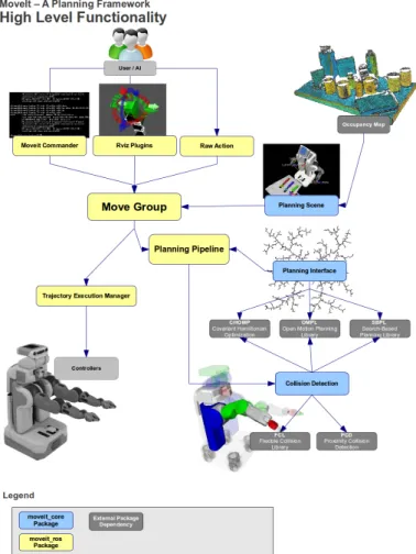
3.4.2 MoveIt! - motion planning framework . . . 49
3.5 ROS-Vehicle Communication . . . 57
3.5.1 Mavlink Protocol . . . 57
3.5.2 MAVROS - a ROS-Mavlink bridge . . . 58
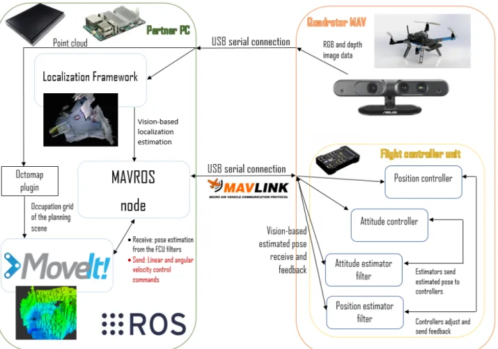
3.5.3 System architecture . . . 58
3.5.4 Mavconn – the decoder between ROS and MAVLink . . . 59
3.5.5 Nodelib – MAVROS core . . . 60
3.5.6 Plugin library . . . 60
4 Results 63 4.1 Tests specificities . . . 63
4.1.1 Testing area . . . 63
4.1.2 Localization modules parameters . . . 65
4.1.3 FCU estimators parameters . . . 66
4.1.4 Datasets . . . 67 4.2 Localization results . . . 67 4.2.1 Time performance . . . 68 4.2.2 Localization performance . . . 70 4.3 Mapping performance . . . 77 5 Conclusions 79 5.1 Achievements . . . 80 5.2 Future Work . . . 80
Bibliography 84
A Frame conversions 85
B Results support images 87
B.1 Used AR markers . . . 87 B.2 Presented results plot perspectives . . . 88
List of Tables
4.1 Datasets description . . . 68 4.2 Localization frameworks mean working rates on the laptop . . . 69 4.3 Localization frameworks mean working rates on the Odroid-U3 . . . 70 4.4 Localization frameworks time performance evaluation on the laptop and on the Odroid-U3 70 4.5 DEMO without sensor fusion VS Ground truth mean errors . . . 71 4.6 CCNY RGBD without sensor fusion VS Ground truth mean errors . . . 71 4.7 Comparison between each localization framework without sensor fusion against ground
truth . . . 73 4.8 DEMO with sensor fusion VS DEMO without sensor fusion mean errors . . . 73 4.9 DEMO with sensor fusion VS Ground truth mean errors . . . 74 4.10 CCNY RGBD with sensor fusion VS CCNY RGBD without sensor fusion mean errors . . 74 4.11 CCNY RGBD with sensor fusion VS Ground truth mean errors . . . 74 4.12 Comparison between each localization framework with sensor fusion against ground truth 75 4.13 Comparison between localization estimation mean absolute error with and without fusion
of optical flow measurements . . . 76 4.14 DEMO without sensor fusion on the Odroid VS Ground truth mean errors . . . 76 4.15 CCNY RGBD without sensor fusion on the Odroid VS Ground truth mean errors . . . 77
List of Figures
1.1 Types of vehicles comparison . . . 3
2.1 Quadrotor MAV used in this project . . . 7
2.2 Inertial frame . . . 8
2.3 Body frame . . . 9
2.4 Vehicle frame . . . 9
2.5 Altitude increase . . . 11
2.6 Vehicle roll movement . . . 11
2.7 Vehicle pitch movement . . . 12
2.8 Vehicle yaw movement . . . 12
2.9 Graph-based SLAM architecture . . . 16
2.10 Concept applied to quadrotor movement . . . 19
2.11 Feature tracking example . . . 20
2.12 A simple complementary filter . . . 24
2.13 Complementary filter applied to noise . . . 25
2.14 Inertial navigation complementary filter . . . 25
2.15 Second-Order Complementary Filter for Inertial Navigation . . . 26
2.16 Raw point cloud . . . 28
2.17 A voxel grid generated from an object observation . . . 28
2.18 Elevation map of an observed tree . . . 29
2.19 Elevation grid of an observed tree . . . 29
2.20 Octmap representation of a building . . . 30
2.21 Octree decomposition in multiple cubes . . . 30
2.22 Attitude controller . . . 33
2.23 PID controller . . . 33
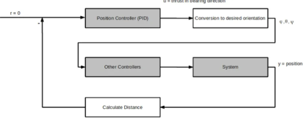
2.24 Full loop control scheme . . . 34
2.25 RRT tree representation . . . 35
2.26 PRM graph representation . . . 36
2.27 KPIECE multi-level grid . . . 36
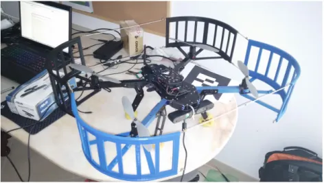
3.2 Customized quadorotor used on this project . . . 41
3.3 Asus Xtion Pro Live . . . 41
3.4 PX4Flow kit . . . 43
3.5 HRLV-EZ Ultrasonic Range Finder . . . 43
3.6 Used laptop . . . 44
3.7 Odroid U3 board . . . 44
3.8 FCU position controller flowchart . . . 46
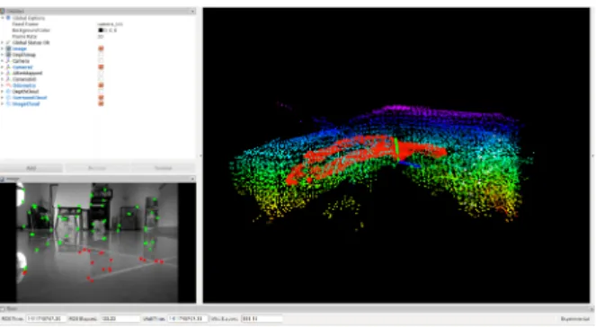
3.9 RGBDSLAM GUI . . . 48
3.10 DEMO RGBD transformations and mapping on Rviz . . . 49
3.11 CCNY RGBD transformations and mapping on Rviz . . . 49
3.12 MoveIt! framework high-level architecture . . . 50
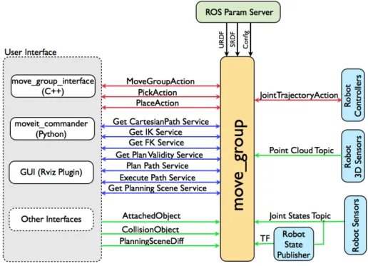
3.13 System architecture . . . 51
3.14 MoveIt! mapping capabilities being shown on Rviz . . . 53
3.15 Planning Pipeline . . . 54
3.16 MoveIt! Setup Assistance with MAV created model . . . 56
3.17 Mavlink packet . . . 57
3.18 MAVROS System Architecture . . . 59
4.1 Indoor tests area . . . 64
4.2 Outdoor tests area . . . 65
4.3 Localization frameworks time performance on the laptop . . . 68
4.4 Localization frameworks time performance on the Odroid-U3 . . . 69
4.5 RGBD SLAM estimated path and map presented on GUI . . . 72
4.6 Original image stream . . . 77
4.7 Different occupation grid resolutions for the same image stream . . . 78
A.1 Coordinate frame conversions for local ground frame . . . 86
B.1 AR Markers used on the simulated Ground Truth system . . . 87
B.2 DEMO estimated localization without fusion VS Ground truth . . . 88
B.3 DEMO estimated localization without fusion VS Ground truth - perspectives . . . 88
B.4 CCNY RGBD estimated localization without fusion VS Ground truth . . . 89
B.5 CCNY RGBD estimated localization without fusion VS Ground truth - perspectives . . . . 89
B.6 RGBD SLAM estimated localization without fusion VS Ground truth . . . 90
B.7 RGBD SLAM estimated localization without fusion VS Ground truth - perspectives . . . . 90
B.8 DEMO estimated localization with fusion VS without fusion . . . 91
B.9 DEMO estimated localization with fusion VS Ground truth . . . 91
B.10 DEMO estimated localization with fusion VS Ground truth - perspectives . . . 92
B.11 CCNY RGBD estimated localization with fusion VS without fusion . . . 92
B.13 CCNY RGBD estimated localization with fusion VS Ground truth - perspectives . . . 93 B.14 DEMO estimated localization without sensor fusion on the Odroid . . . 94 B.15 DEMO estimated localization without sensor fusion on the Odroid VS Ground truth -
per-spectives . . . 94 B.16 CCNY RGBD estimated localization without sensor fusion on the Odroid . . . 95 B.17 CCNY RGBD estimated localization without sensor fusion on the Odroid VS Ground truth
- perspectives . . . 95 B.18 Comparison between localization estimation with and without optical flow measurements
Abbreviations
ARM Advanced RISC Machine
COM Computer-On-Module
CRC Cyclic redundancy check
DOF Dimensions of freedom
EKF Extended Kalman Filter
ENU East-North-Up
ESC Electronic Speed Controller
FCU Flight Control Unit
FPV First Person View
GPS Global Positioning System
iSAM Incremental Smooth and Mapping
IMU Inertial Measurement Unit
ISR Intelligence, Surveillance and Reconnasissance
ITU International Telecommunication Union
KLT Kanade-Lucas-Tomasi feature matching
KPIECE Kinodinamic Planning by Interior-Exterior Cell Exploration
MAV Micro Air Vehicle
PID Proportional-Integral-Derivative
QVGA Quarter Video Graphics Array
NED North-East-Down
ORB ORiented Binary robust independent elementary features
PRM Probability RoadMap
RANSAC Random Sample Consensus
RGB-D Red, Green, Blue - Depth
ROS Robot Operating System
RPM Remotely piloted vehicles
RPY Roll, Pitch, Yaw
RRT Rapidly Exploring Random Trees
SIFT Scale-invariant feature transform
SLAM Simultaneous Localization and Mapping
SURF Speeded-Up Robust Features
SXGA Super Extended Graphics Array
sUAS small Unmanned Aircraft System
TOF Time-Of-Flight
UAV Unmanned Air Vehicle
UTM Universal Transverse Mercator
Chapter 1
Introduction
1.1
Motivation
A MAV system capable of doing autonomous navigation in confined areas still is a challenge to the researchers and designers that are looking to create a reliable and during system, given that there are many variables that come to the challenge.
Since the starting issue of this kind of systems is the localization, and so that this work can be contin-ued in the future, a pre-framework/hardware selection process and a comparison between the existent state-of-the-art localization is indeed needed, so to evaluate its performance on the pose estimation of the quadrotor, and it can properly be forwarded to a framework that, in combination with the mapping capabilities, can perform the planning of a path issued by the user in a static environment, where the volume occupation of the obstacles and the localization of the MAV is known.
1.2
Objectives and Contributions
The global objective of the work done for this thesis is to provide a system able to navigate autonomously a micro-air vehicle, more specifically, a quadrotor, within a 3D environment that is being online recon-structed using data from a RGB-D sensor mounted on-board the quadrotor. The particular goal for the thesis itself is to prepare a system for the navigation task, resulting from the integration of different subsystems, having as a milestone provide a consistent comparison of different localization frameworks and testing the mapping capability inside a subsystem that is able to, after receiving localization of the vehicle and mapping from the environment, can proceed to navigation.
The navigation and path planning tasks will be active based on the estimated pose of the vehicle relative to the constructed map given by the sensor fusion of the main sensors aboard the quadrotor: a 10DOF IMU together with an RGB-D camera and a facedown Optical Flow with Sonar unit to give a 3D pose and velocity estimate of the quadrotor.
The discussion from the theoretical point of view will focus primarily on the state-of-the-art methods for vision-based localization and three-dimensional reconstruction of an environment. Navigation
algo-rithms that can be used to control of the quadrotor will also be summarily described, since the main point of attention was given to the localization and mapping issues.
From the practical point of view, instead, the ultimate goal will be the realization of a system able to autonomously fly a quadrotor within an environment that is online reconstructed in a map. For that, a comparison between different localization algorithms is done, so that the performance of both can be compared in terms of localization and time. The navigation task, which was already proved to work in a simulation environment, was already prepared to be tested in this framework, but it will be forwarded for future work.
Since the purpose is not to create new solutions to this matter, some open-source solutions are used and integrated to get a localization and mapping system working, so it can serve as a starting point and test bench for future algorithms and implementation works, not only in this tasks, but also to allow advancing to navigation tasks.
1.3
State-of-the-art
Small Unmmaned Aircraft Systems (sUAS), or usually called MAVs (micro aerial vehicles), are UAV’s with most of the capabilities of large UAV’s but with smaller footprints. Are the most common type of UAV’s since they are also already present in the R/C community and already have several civilian applications besides the common military ones for which they were already used.
One of the primary applications for a sUAS is for ISR (Intelligence, Surveillance, and Reconnais-sance), but there are many applications. Some examples include: determining the direction a fire is moving on hot spots, monitoring a forest for new fires, scouting dangerous areas (situational aware-ness), aiding the pursuit of suspects, intruder detection/security, search and rescue (SAR) (especially in inaccessible areas), inspecting tall objects (towers to find damage, eagles nests to count eggs), finding invasive plants, counting endangered wildlife, surveillance of pipelines or high tension lines or volcanoes, accident report assistance, real time mapping, mapping with Colour Infrared (CIR), Short Wave Infrared (SWIR), Long Wave Infrared (LWIR), cameras and environmental testing for radiation and chemical leaks, just to name a few.
The common type of these vehicles are the remotely piloted vehicles (RPV), which are UAV’s that are stabilized and have sensors, but do not operate with an autopilot. Some of them are equipped with what is called FPV (first person view), which allows the pilot to fly by monitoring a camera mounted on the aircraft. Both RPV and FPV are complementary to sUAS because UAS seldom fly completely autonomously, especially during take-off and landing, when we are considering outdoor vehicles.
sUAS primarily are divided into two type of vehicle categories: the multirotors (Figure 1.1 (a)) and fixed wing (Figure 1.1 (b)). Given that this work has as its focus on indoor navigation, the primary focus will be on the first ones, since the fixed wing are usually bigger vehicles and the type of flight made is not adequate for indoor flights.
Autonomous MAVs (micro aerial vehicles), primarily multirotors, are getting more and more attention within robotics research, since their applications are tremendous. One of them is easily identified: SAR
(a) Multirotor (b) Fixed Wing
Figure 1.1: Types of vehicles comparison
[11] in inaccessible areas, where a common pilot will not have access (a FPV system in this case is impossible to use given that the signal, for example, in a mine, will be lost).
From all multirotor types, a quadrotor MAVs is an ideal choice for autonomous reconnaissance and surveillance because of their small size, high manoeuvrability, and ability to fly in very challenging envi-ronments. In any case, for getting true autonomy, a MAV must neither rely on external sensors (i.e. an external tracking system) or on off-board processing to an external computer for autonomous navigation. To perform these tasks effectively, the quadrotor MAV must be able to do precise pose estimation, navigate from one point to another, map the environment, and plan navigation and (if able) exploration strategies. Ideally, all these processes have to run on-board the MAV, especially in GPS-denied envi-ronments.
One of the most essential problems for autonomous MAVs is localization or pose estimation. Com-mon ground robots can just stop and wait for its pose estimate but a MAV typically cannot do it. In order not to crash, it needs reliable pose estimates in 6D (position and orientation) at a high frequency. If the autonomous MAV should also be able to navigate in previously unknown environments, it has to solve the SLAM (simultaneous localization and mapping) problem.
Many research projects targeted some of these abilities using different kinds of technologies. One of those is using laser range finders [4, 11, 30, 47], which usually is an expensive piece of device given that it gives good range and precision. Other technology can be the use of artificial markers [8, 13]. Common sense says that this is can be used on a lab environment but in a real world situation, we will not have markers everywhere so the MAV can position itself and navigate. Same thing with motion capture systems like VICON [24, 38] or OptiTrack [23]. They are extremely expensive systems with the highest precision of all the technologies that can be used, but again, they are expensive and the world does not have those system cameras spread everywhere. Other systems like [49] use low cost sensors, but that mean a lower precision on the vehicle localization.
On evaluating this systems, we see that the own sensors becomes an impediment factor when designing a MAV that can achieve fully autonomy in mapping and/or exploration. The primary disruptive facts are the weight and the power consumption, where an equilibrium must be found to potentiate both autonomy and reliability of the system.
external processing units, which removes its complete autonomy. That is the case of using an external global positioning system, like a motion capture system. Or it is a heavy system with a heavy payload, which turns out to be a less flexible vehicle, with a higher power consumption. An example of it is using a laser range finder, which considerable weight and power consumption pose a problem for MAVs with stringent payload and power limitations.
Projects with RGB-D cameras [5, 29, 46], i.e. cameras that provide registered colour and depth images, seem to be the perfect approach for the indoor navigation task: They are small, light-weight, and provide rich information in hardware already, without requiring additional expensive post processing computations by the on-board computer, like stereo cameras do [20, 53]. Still, the applications in [5, 29, 46] lack a general explanation on how to transpose to a usable open-source system. [5] uses a very expensive platform to get the job done.
The processing power also becomes an issue when designing this kind of systems. Usually, a system that relays on external processing power does not have problems regarding this variable, since weight is reduced and the higher power consumption is on the external system. But that means that the system itself it is not self-dependent, relaying on an external system so it can localize itself and proceed with its autonomous behaviour. In the other hand, adding higher processing units to the MAV itself may be the best solution, but then it must be found a balance between the processing power, the weight of the processing unit and the power consumption.
Embedded platforms capable of supporting Linux type of OS are, right now, a great success among the creative and researching community. Their high processing capabilities, low weight and footprint and low power consumption allows great usage on robotics projects, especially when weight and flexibility of the system are essential for its proper work, which is the case of MAVs.
For understanding how this can be achieved, localization and mapping must be divided into two different problems and then combined in a structured way.
The problem of localization can be solved by visual odometry if complemented with a proper cor-rection [10, 28, 45, 48], given that it accumulates error. In case of ground robots, this odometry can be measured by the use of the odometry of the wheels. In the case of aerial robots, since they do not have wheels, a different type of odometry must be used. Since cameras can be used as sensors, visual odometry is the common approach for robot localization, since it allows the egomotion estimate using as input single like in [10, 21, 28] or multiple cameras like in [20, 53].
Mapping, on the other hand, is a different issue. Many robotics applications require a three-dimensional map of the environment that surrounds them created from the data recorded by sensors. But, to create and maintain this amount of data in an efficient manner is not a trivial operation, so a good method of management of the map should ensure the ability to model free space, occupied and not yet ex-plored, quick and easy creation and update of it, representation of the information in a probabilistic way, efficiency and multi-resolution.
The combination of map with 3D info of the environment and the localization process given by visual odometry or SLAM give a full 6D estimation of the robot pose and motion, which can be forward for to a motion planning framework that allows a structured navigation of the vehicle in the environment.
1.4
Thesis Outline
So to understand the work done in this project, the following lines give a short description of what is addressed in each chapter.
In Chapter 2 are reviewed the basic concepts to quadcopters and its physics model and functioning, followed by a review methods of SLAM (graph-based SLAM, visual odometry, feature handling, bundle adjustment and graph optimization, pose estimation and sensor fusion), optical flow, mapping, navigation and path planning.
Chapter 3 is where the development part is stated. It presents the vision-based localization, mapping and navigation modules used and the conceptual solutions for the initial problems given. It presents an overview of the used software and hardware, which includes the quadrotor platform and configuration used, the external and inboard sensors and the integrated software framework used to build the system. Also, it is explained the module to communicate between the FCU and the computer.
The forth chapter focus on testing the localization and mapping modules on different test conditions and presenting its results.
Chapter 2
Theoretical Background
This chapter presents the theoretical background behind the frameworks used on the project. It starts with an overview over the vehicle mathematical model, then follows with the explanation of some of the algorithms and techniques used for localization, mapping and that may be used for navigation.
2.1
Vehicle model
This subchapter regards an explanation of the vehicle being used, the coordinate frames used and the kinematics and dynamics mathematical models.
2.1.1
Introduction
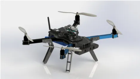
A MAV, or more specifically, a quadrotor MAV, is a rotary wing aircraft with four motors/propellers located at the ends of a cross structure (Figure 2.1), with the same control capabilities as helicopters.
Figure 2.1: Quadrotor MAV used in this project
In contrast to helicopters, they stand out by virtue of their much simpler and thereby massively less sensitive mechanics. There are four motors, which are rigidly connected with two right and two
left-rotating propellers. They also differ from other multirotor UAV given that they are more flexible in manoeuvring than any of the others: tricopters are flexible, but their control is harder, and cannot carry much of a payload. Hexarotors and beyond can carry a larger payload, but are less flexible on movement. The flight behaviour of a quadrotor is determined by the rotation speeds of each of the four motors, as they vary in concert, or in opposition with each other, which define their attitude and steering mechanism. Doing its mathematical model allows defining a good description of the behaviour of a system, which can be used to predict the position and orientation of the quadrotor. The last can further be used to develop a control strategy, whereby manipulating the speeds of individual motors results in achieving the desired motion.
Defining a full mathematical model requires the definition of the vehicle kinematics, which regards the aspects of motion (position and orientation), providing a relation between vehicle’s position and velocity, and the vehicle dynamics, which regards the application of forces that influence accelerations and, consequently, the vehicle motion.
2.1.2
Coordinates Reference Frames
Before moving, it is essential to it to specify the adopted coordinate systems and frames of reference and also how transformations between the different coordinate systems can be made.
There are three main frames to be considered [43]:
1. Theinertial frame, which regards an earth-fixed coordinate system with the origin located on the
ground, which usually is the local origin of the system when it starts, or can be defined by the user (using a position triplet of X,Y ,Z coordinates or GPS coordinates). The representation is in Figure 2.2.
Figure 2.2: Inertial frame
2. Thebody frame has its origin located at the centre of gravity of the vehicle and as an alignment
that considers the X-axis in the direction of the first motor and the Y -axis along the direction of the second motor. The Z-axis is where the cross product ZB = XB× YB happens. The representation is
in Figure 2.3.
3. Thevehicle frame is the inertial frame but with the origin on the centre of mass of the vehicle, but
can have two possible configurations, depending if we consider a ”X” type of motion or a ”Plus” (+) type. The ”Plus” configuration has the X and Y of the vehicle frame aligned with the X and Y of the body frame, while with the ”X” configuration, there is a yaw rotation, where the X-axis of the vehicle points in the direction of the midline between the two front motors. The representation is in Figure 2.4.
Figure 2.3: Body frame
Figure 2.4: Vehicle frame
2.1.3
Kinematics
Let ρI = [xI, yI, zI]T and ΘT I = [φ
I, θI, ψI]T be the position in Cartesian coordinates and orientation
(roll, pitch and yaw, which are the rotations around x, y and z-axis) of the vehicle relative to the inertial frame, respectively. Consider pose χI as = (ρI, ΘI), i.e the combination of the position and orientation.
While the position of the vehicle is defined in the inertial frame and the velocity of the vehicle is defined on the vehicle frame, which it will be considered equal to the body-frame for simplicity, a rotation matrix must be defined so a frame transaction must occur. Then, considering νV = (Υ, ω), where
ΥV = [vx, vy, vz]T is the linear velocity and ωV = [rr, pr, yr]T the angular rates of roll, pitch and yaw,
relative to the vehicle frame, we get the following rotation matrix for the three Euler angles [35, 37]:
R(ψ) = cosψ −sinψ 0 sinψ cosψ 0 0 0 1 , R(θ) = cosθ 0 sinθ 0 1 0 −sinθ 0 cosθ , R(φ) = 1 0 0 0 cosφ −sinφ 0 sinφ cosφ , (2.1)
which combination, RΘ= cosψ −sinψ 0 sinψ cosψ 0 0 0 1 . cosθ 0 sinθ 0 1 0 −sinθ 0 cosθ . 1 0 0 0 cosφ −sinφ 0 sinφ cosφ , (2.2)
corresponds to the final rotation matrix:
RΘ= cψcθ cψsθsφ− sψsφ sψsφ+ cψsθcφ sψcθ cψcφ+ sψsθsφ sψsθsφ− cψsφ −sθ cθsθ cθcφ , (2.3)
where cα ≡ cosα and sα ≡ sinα. Given this rotation matrix, it’s now possible to get a relation between
the position vector ρI and the linear velocity vector ΥV with,
˙ ρI = R ΘΥV ⇔ ˙ x ˙ y ˙ z = RΘ vx vy vz . (2.4)
And given the same process, it is done the same thing to the angular position and velocities, which gives the relation:
ωV = TΘ−1Θ˙I ⇔ ˙ΘI = TΘωV, (2.5)
where TΘis a transformation matrix. This one is calculated through:
rr pr yr = TΘ−1 ˙ φ ˙ θ ˙ ψ = ˙ φ 0 0 + Rφ−1 0 ˙ θ 0 + Rφ−1Rθ−1 0 0 ˙ ψ , (2.6)
which, after inverting, we will get the following transformation matrix [12]:
TΘ= 1 sφtθ cφtθ 0 cθ −sφ 0 sφ/cθ cφcθ , (2.7) where tα≡ tanα.
2.1.4
Dynamics
Considering the angular velocities of the four motors as a vector ω = [Ω1, Ω2, Ω3, Ω4]T [15]. The four
types of movement control will be described as a U vector, where U1≡ altitude, U2≡ roll, U3≡ pitch
and U4 ≡ yaw. So to be able to get the corresponding attitude change, the input for each motor must
be changed accordingly. For this particular case, it will be considered a ”cross” (X) type of motion to the quadrotor, since the used quadrotor in the project was designed for this type of motion, which means
the first motor Ω1is the top left motor and the rest is numbered in a clockwise way.
So, if one wants to change its altitude U1[N ], all four motors must change their angular velocity at the
same time, as we can see in Figure 2.5.
Figure 2.5: Altitude increase
The rolling movement U2[N.m] is obtained by increasing/decreasing the pairs Ω1, Ω4 and Ω2, Ω3,
which depends if one wants to bend right (Fig. 2.6(a)) or left (Fig. 2.6(b)) respectively, which will change the φ angle.
(a) Move vehicle left (b) Move vehicle right
Figure 2.6: Vehicle roll movement
The pitching movement U3[N.m] is obtained by increasing/decreasing the pairs Ω1, Ω2 and Ω3, Ω4,
which depends if one wants to bend backward (Fig. 2.7(a)) or forward (Fig. 2.7(b)) respectively, which will change the θ angle.
The yaw movement U4[N.m]is obtained by increasing/decreasing the pairs Ω1, Ω3and Ω2, Ω4, which
depends if one wants to turn right (Fig. 2.8(a)) or turn left (Fig. 2.8(b)), respectively, changing the ψ angle.
(a) Move vehicle backward (b) Move vehicle forward
Figure 2.7: Vehicle pitch movement
(a) Rotate vehicle right (b) Rotate vehicle left
Figure 2.8: Vehicle yaw movement
To consider forces and moments, the Laws of Newton must be applied [7, 12]. Considering Newton’s second law, applied to the translational motion,
FV = m( ˙ΥV + ωV × ΥV),
(2.8)
and to rotational motion,
τV = I ˙ωV + ωV × (IωV),
(2.9) with m equals the vehicle mass in kilograms, ˙ΥV the linear acceleration in meters per second squared,
˙
ωV the angular acceleration in radians per second squared, I a diagonal matrix which is the inertia
it is assumed a symetric configuration on the vehicle X and Y axis: I = Ixx 0 0 0 Iyy 0 0 0 Izz . (2.10)
Just to complete the equations 2.8 and 2.9, it’s defined the system entrance UV vector and added the
gravity force. That will result in a new set of equations, after some empirical deductions:
FV = RTΘ. 0 0 −mg + 0 0 U1 = mgsθ −mgcθsφ −mgcθcφ + 0 0 U1 = mgsθ −mgcθsφ −mgcθcφ + 0 0 b(Ω2 1+ Ω22+ Ω23+ Ω24) , (2.11) τV = τV x τyV τzV = U3 U3 U4 = bl(Ω2 1+ Ω24− Ω22− Ω23) bl(Ω23+ Ω24− Ω2 1− Ω 2 2) d(Ω22+ Ω24− Ω21− Ω23) . (2.12)
The combination of the kinematics equations 2.4 and 2.5 with 2.11 and 2.12 gives the complete mathe-matical model of the quadrotor:
˙ X ˙ Y ˙ Z = RΘ vx vy vz , (2.13) ˙ φ ˙ θ ˙ ψ = TΘ pr rr yr , (2.14) ˙vx ˙vy ˙vz = yrvy− rrvz rrvz− yrvx prvx− rrvy + g sθ −cθsφ −cθcφ + 1/m 0 0 U1 , (2.15) ˙rr ˙ pr ˙ yr = Iyy−Izz Izz pryr Izz−Ixx Iyy rryr Ixx−Iyy Izz rrpr + 1 IzzU2 1 IyyU3 1 IzzU4 , (2.16) U1 U2 U3 U4 = b(Ω21+ Ω22+ Ω23+ Ω24) bl(Ω2 1+ Ω24− Ω22− Ω23) bl(Ω2 3+ Ω24− Ω21− Ω22) d(Ω2 2+ Ω24− Ω21− Ω23) , (2.17)
where g is the gravity acceleration in [m.s−2], b is the propulsion coefficient in [Kg.m.rad−2], d is the
binary coeficient of the propellers in [Kg.m2.rad−2]and l is the distance from the centre of the quadrotor
2.2
Localization
In the next sections, it is covered important aspects of pose estimation for robots, including the different concepts involved on visual odometry and visual graph-based SLAM algorithms, what is optical flow and how it aids on robot localization, and finally how can data from different sensor sources be merged into sensor fusion algorithms so that vehicle pose and motion can be predicted.
2.2.1
Introduction
In order to localize itself, a robot has retrieve both relative and absolute data measurements that provide feedback about the robot actions and the situation of the environment that surrounds it. The main issue usually falls on how the robot deals with noisy and unpredictable data that can distort the way the world is presented and how the vehicle is behaving.
Vehicle localization issue is a key problem when making autonomous robots, since it can be difficult for a robot to determine what to do next if it does not know where it is. There are many types of technologies and sensor sources available for robot localization, including GPS, odometry, active and passive beacons, sonar, among others, but improving one of them may imply more costs and additional processing power. That is why adding different cheap sensor sources and fuse them in some filter is the best and the usually adopted solution for localization and, consequently, for navigation.
Regarding the measurements, there are many types of sensors that provide positioning and distance data for the robot know how the environment is composed, is form and distances, the presence of obstacles, etc. All that data must be used in a way that the robot can plan, for example, its movements given the presence of dynamic entities and the dimensions of a given area. Also, besides its position, the robot must be aware of its attitude and motion, so a proper sensor measurement that, after its processing in a filter, can give a velocity estimation of the vehicle movement, is indeed welcoming. In this last case, optical flow algorithms are a way of determining the motion of the vehicle given image processing of camera streams.
In the last paragraph, the word “filter” was also used as a way of processing data. When we discuss filters in terms of robot localization we are considering sensor data filters that allow the fusion of different sensor sources to estimate the pose and motion of a robot in a given environment. The use of filters allows the improvement of the estimations besides giving a continuous estimation even if a sensor source fails. It also deals very well with the noise of the sensors by interpolating the data of different sensor sources on a probabilistic mathematical model.
2.2.2
Visual Odometry alone vs SLAM
Visual odometry is a type of method available in mobile robots that allows the pose and attitude estima-tion of the vehicle based on the data retrieved from cameras.
In the other hand, SLAM, or simultaneous localization and mapping, regards the pose estimation of the robot given the global estimate in relation with a map, which implies a incrementally map
reconstruc-tion and posireconstruc-tioning relative to that map.
Visual odometry mainly aims at recovering the path incrementally, pose after pose, and potentially optimizing only over the last n poses of the path, estimates local motion and generally has unbounded global drift, which differs from SLAM, which in general wants to obtain a globally consistent estimate of the robot path [51]. That implies keeping a track of a map of the environment because it is needed to realize when the robot returns to a previously visited area, which is a process called loop closure. In any case, a SLAM algorithm requires the use of feature extractor and matching algorithms from image streams coming from vision sensors (considering visual SLAM algorithms), which are also present on the visual odometry algorithms.
In order to understand how each type of pose estimation methods work and have to offer, in the next sections, some basic concepts and techniques will be presented, mainly regarding the techniques used and tested on the project developed for this thesis.
Graph-based SLAM
If the autonomous MAV wants to able to navigate in previously unknown environments, it has to per-form SLAM, which is an acronym for simultaneous localization and mapping. SLAM has been one of the major fields of research in mobile robotics during the past decades and it gives the ability to the robot to understand and perceive the unknown environment while moving through it and, at the same time, incrementally build a map of what has been explored, on which simultaneously determines its localization.
The solution of the SLAM problem has been one of the notable successes of the robotics community given the last researches of the robotics fields. It has been formulated and solved as a theoretical problem in a number of different ways and has also been implemented in a number of different research areas and applications as indoor robots, outdoor, air and underwater systems and, as is, it can be considered a solved problem.
However, some issues remain in practically implement a more general SLAM solutions and that can use perceptually rich maps as part of the algorithm itself. For this last issue, RGB-D cameras can be used. They provide both colour images and per-pixel depth estimates, which richness of data and the recent development of low-cost sensors have been combined on an excellent opportunity for mobile robotics research [20], which also include MAV’s.
The three main approaches to the SLAM problem consider: firstly, a filter approach solution, which use a Kalman Filter to estimate the robot pose; secondly, also a filter solution, but using the so called Monte Carlo solution, or Particle Filter; the third approach, which is the one that is going to be consider in this project given the used algorithms, is the graph-based SLAM solution.
The graph-based SLAM [22] describes the robot localization as a graph, where every node cor-responds to a robot position and to a sensor measurement and the edges between two nodes are considered data-dependent spatial constraints between the two nodes. This constraints are obtained from observations of the environment or from movement actions carried out by the robot.
config-uration of the nodes that is considered, by the several iterations, mostly consistent with the raw mea-surements being modelled by the edges, with this last ones being seen as “virtual meamea-surements”. The modulation of the graph is consistent with a probabilistic model, where the edges have the probability of a given pose of the robot given the relative measurements of the nodes with which it is connecting.
A graph-based SLAM is usually divided into three main modules, each one with its proper function: the frontend framework, the backend framework and the map representation.
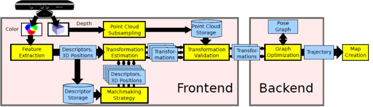
In the case of RGBD SLAM1, or in the case of CCNY RGBD Tools2, which is very similar, the structure
of the graph-based SLAM architecture is based on the schematic of Figure 2.1 [14]. CCNY RGBD though lacks a backend framework, as explained in 3.4.1.
Figure 2.9: Graph-based SLAM architecture
As said, there are three main components of the framework. The frontend framework includes all the sensor data processing that allow the generation of specific geometry relations between the data being received, which includes feature detection, extraction and matching. This also includes a way of dealing with motion between two observations, which requires a visual odometry algorithm to deal with it.
In the case of the algorithms that uses RGB-D data, as in the case of the SLAM frameworks used on this project, that means having a way of determine landmarks by extracting a high-dimensional descriptor vector from the image data and store it together with their location relative to the observation pose. The depth info is then used as a way of validate the transformations between the camera link and the 3D descriptors being retrieved by the feature extraction algorithms being used.
To deal with uncertainties introduced by sensor measurements, it is used a graph that represents the geometric relations and their uncertainties, which can then be optimized in the backend using graph optimization techniques, allowing to obtain a maximum likelihood solution for the represented robot trajectory.
Monocular visual odometry
Visual odometry is implemented in algorithms nowadays that allow the use of different kinds of image processing techniques, depending on the current used sensor and what type of features can be used, to allow the robot to localize itself on the environment. The idea is to compute and retrieve the egomotion
1F. Endres. RGBDSLAM v2.http://felixendres.github.io/rgbdslam_v2. Online. 2ROS Wiki. CCNY RGBD Tools. http://wiki.ros.org/ccny_rgbd_tools. Online.
based on the features being retrieved and matched, and the relation between the same features from one image to another.
In specific to a MAV system like this, it is recommended the use of an algorithm that is able to be relatively robust but that can assure processing at high rates, which most of the current online image processing techniques for motion perception and localization are not, given the higher processing re-quired so they can work, which usually means using an external processing unit for the data stream or the use of high power consumer COM.
There exists two types of visual odometry algorithms based on the type/number of cameras being used: the monocular visual odometry, which can use a typical camera with just one oculus to process the egomotion, or stereo visual odometry, which uses a special camera with two or more oculus or, instead, multiple cameras with image merging.
The approach used on this project, and since it is specifically used and RGB-D type of camera, uses a monocular visual odometry algorithm that adds depth data to improve the pose estimation. One of the methods used on it is explained in 2.2.4. section.
2.2.3
Optical Flow
Optical flow is the pattern of apparent motion of image objects between two consecutive frames caused by the movement of an object or camera3, resulting on a 2D vector field where each vector is a displace-ment vector showing the movedisplace-ment of points from a frame to the other. This vector is a result of the calculation of partial derivatives with respect to the spatial and temporal coordinates.
The used methods allow the estimation of motion as either instantaneous image velocities or discrete image displacements in a sequence of ordered images. That is why it is very useful on robot appliances since it allows the egomotion estimation of the robot given the estimated velocity of pixels from a frame to another in a image stream.
The most known methods to give the solutions to the optical flow equations are the Lucas-Kanade method [42], which obtains the solution of the optical flow equations by assuming a constant value of flow for each neighbours of a certain pixel and calculating the neighbour flows iteratively by a least squares approximation, and the Horn-Schunck method [42], which applies a constant value of smoothness in all the pixels, represented by a energy function, so to minimize distortions and choose the solutions for the flow equations which give more ”smoothness”.
Metric velocity calculation
For consideration of what is used in this project, it is going to be explained how the optical flow module being used gives an estimate of 3D velocity of the camera frame relative to the image plane, based on the work developed in [26].
3OpenCV 3.0 dev doc. Optical flow. http://docs.opencv.org/trunk/doc/py_tutorials/py_video/py_lucas_kanade/py_
Assuming P = X Y Z , (2.18)
as a point in the camera reference frame, the Z-axis being the optical axis, f the focal length and the centre of the projection as the origin of the frame. The pixel coordinates projected in the image plane are represented by
p = fP
Z. (2.19)
Given that the focal length gives the distance between the origin and the image plane, that results on a coordinate p = x y z , (2.20)
which is constant. The relative motion can then be computed with the equation
V = −T − ω × P, (2.21)
with ω being the angular velocity and T the motion translational component. Applying the derivative with respect to time will give a relation to the velocity of P (in camera frame) and velocity of p (in image plane). The result of that relation is then applied and the result is the motion field equations:
vx= Tzx − Txf Z − ωyf + ωzy + ωxxy − ωyx2 f , (2.22) vy= Tzy − Tyf Z − ωxf + ωzx + ωxy2− ωyxy f . (2.23)
Since the motion field is composed by a translational part plus a rotational part, but given that rotational parts are Z-independent, the translational component can be calculated using the focal length f and the distance to plane Z, assuming that the rotational velocity is zero or it is compensated by a calculation of a gyroscope measurement:
vtrans= v
Z
f. (2.24)
In the case of a constant distance to the plane, it is considered
vx= −Txf Z − ωyf + ωzy, (2.25) vy= −Tyf Z − ωxf + ωzx, (2.26)
where terms divided by the focal length are ignored given that the order of magnitude is smaller com-pared with the other terms. Having the angular rates given by a gyroscope measurements, the previous velocities can be compensated, assuming the considered ignored terms.
An idea of how this calculations apply to a MAV movement is described on Figure 2.104.
Figure 2.10: Concept applied to quadrotor movement
2.2.4
Feature handling
Feature handling is an essential part of image processing which deals with the detection and representa-tion of interesting parts of an image or a stream of images into usable compact data vectors. In the case of vision-based localization systems, it is essential to have techniques that allow detection, extraction and matching of the computed features, so to allow the robot to localize and estimate its motion given the data being processed by its camera sensors.
There are various methods that can be used for this purposes, but the next section will cover the one used in feature extraction and matching on the SLAM frameworks used on this thesis: SURF [6]. In the case of the visual odometry framework, it is used the Kanade-Lucas-Tomasi [50] for pose estimation, which is allied to the optical flow techniques used for feature tracking but applied to detection and tracking of Harris corners5.
SURF
SURF [6], or Speeded-Up Robust Features, is a method that allows feature detection and extraction. It is based on the descriptors of the images and it is invariant relative to rotation and scale. It proceeds to the detection of the features by firstly, calculating the integral images by
IΣ(x, y) = i≤x X i=0 j≤y X j=0 I(i, j), (2.27)
4APM Wiki. Optical flow sensor. http://copter.ardupilot.com/wiki/optical-flow-sensor. Online.
5OpenCV 3.0 dev doc. Harris corners. http://docs.opencv.org/trunk/doc/py_tutorials/py_feature2d/py_features_
and then applying the previous equation to compute the Hessian Matrix, the convolution over a second order Gaussian derivative [58], for each it calculates the determinant:
H(X, σ) = L(xx)(X, σ) L(xy)(X, σ) L(yx)(X, σ) L(yy)(X, σ) . (2.28)
After that, it uses non-maximum suppression for choosing the local maximums. All the descriptors have a certain intensity content which allows them to be distinguishable. They are computed considering the invariance on rotation, which is obtained by the Haar wavelet on the X and Y directions, and then, after being computed, they are added in the feature vector properly normalized, which adds the invariance on scale.
For feature matching of SURF image descriptors, it can be used some sort of minimization of Eu-clidian distances algorithm, which minimize the distances between each feature. This algorithm can be FLANN [40], brute-force algorithms, among others.
For both of the SLAM frameworks being tested on this thesis, it is used SURF for feature extraction and matching based on brute-force.
KLT feature tracker
The basic idea behind KLT, Kanade-Lucas-Tomasi feature tracker [33, 42, 50] is given a sequence of two grey scaled images, where each pixel has a grey scale value, find a certain value u where the grey scale in the two images is the same, which is represented by the sum of the optical flow of the feature being analysed and the coordinates of the first point.
For that, it is applied a matching function which corresponds to a window where to track those features from a frame to another. The idea is then to find that certain value u that minimizes the matching function.
In the case of the KLT tracker being used on the visual odometry framework, the selected features to track are Harris corners. Figure 2.11 represents an example of some feature points being tracked along a sequence of images [50].
Figure 2.11: Feature tracking example
2.2.5
Bundle adjustment and graph optimization
The idea of bundle adjustment [3] is to find 3D point positions and camera parameters that minimize the reprojection error, formulated as a non-linear least squares problem, given a set of image features and
its relations. It is considered the final step of a optimization/reconstruction problem, and it is very useful for correcting estimations from visual odometry algorithms.
Also, SLAM problems, as in the case of graph-based SLAM, can be optimized using techniques that allow the optimization with the minimization of a non-linear error function that can be represented as a graph.
When the relations between features is a graph, bundle adjustment problem can be treated as a graph optimization problem.
iSAM
iSAM is an approach to SLAM based of fast incremental matrix factorization [39]. Since it is applicable to graph problems, it can also be used in graph optimization problems besides SLAM, such as bundle adjustment problems.
The idea of iSAM is to be used as a graph optimization solution for graph-based problems. It reuses the previously calculated components of the squared root factor of the squared root information ma-trix and performs only calculations over new entries of the mama-trix, which are affected directly by new measurements.
It is also very useful on cases of trajectory loops, where it is used periodic variable reordering of the squared root information matrix so to avoid fill-in of the matrix, which would result on a slowdown of the incremental factor of this type of optimization. Another feature that helps in this last case is use back-substitution as a way of recovering the current estimate.
Gauss-Newton optimization
Considering a minimization of an error function like the following [22]:
F (X) = X
<i,j>∈C
e(xi, xj, zij)TΩije(xi, xj, zij) (2.29)
where X is a vector of parameters that represent the sensor poses, zijthe mean and Ωijthe information
matrix of a constraint between the xiand xjcomputed poses, and e(xi, xj, zij)the vector error function
that computes the difference between the expected observations and the real observation gathered by the robot, i.e. measures how well the poses satisfy the constraint zij.
To solve the minimization equation X = argminxF (X), the Gauss-Newton optimization model can
be applied to find the numerical solution of it. First step is to assume a good initial guess to the robot pose and then apply an approximation to the first order Taylor expansion of this guess. So considering
˘
X as the initial guess,
eij( ˘Xi+ ∆xi, ˘Xj+ ∆Xj) = eij( ˘X + ∆X) (2.30)
' eijJij∆X (2.31)
the error Fij, we get:
Fij( ˘X) + ∆X) = cij+ 2bij∆X + ∆XTHij∆X, (2.32)
where cij ≡ eTijΩijeij,bij ≡ eTijΩijJij and Jij ≡ .JijTΩijJij. After a local approximation, where it is
considered c =P cij, b =P bijand H =P Hij, we obtain,
Fij( ˘X) + ∆X) = c + 2bT∆X + ∆XTH∆X, (2.33)
which can be minimized in ∆X, result of a linear system of the of form ax = b,
H∆X∗= −b. (2.34)
The resulting H matrix is the sparse information matrix of the system. The solution of the linear system can then be given by
X∗= ˘X + ∆ ˘X∗. (2.35)
The Gauss-Newton optimization is then applied, iterating on Eq. 2.33, giving the solution in 2.34 and using 2.35 as an update step, where the previous solution is used as the initial guess of the robot pose.
2.2.6
Pose estimation
The pose estimation is the main core of the vision-based localization frameworks, and allows the esti-mation of both position and orientation of the vehicles, given the camera pose. For what visual pose estimation matters, there are numerous ways of getting the orientation of the visual stream, and those include evaluating the features of the image (or depth data, in case of having this source) and compute the pose of the vehicle relative to that data.
The estimated pose, allied to a proper selection of features and keypoints of the images, also allows to determine the motion of the system, if it is known the motion model of the vehicle given the data being processed.
For the SLAM algorithms being tested in this thesis, there are two main techniques being used for pose estimation: GICP [2] and RANSAC [18].
GICP vs RANSAC
GICP [2], or Generalized Iterative Closest Point, is a generalized model of ICP, which computes the differences, point-to-point, between two point clouds, by applying the a probabilistic model based on Gaussian distributions and using maximum-likelihood estimator to get the transformation between each point cloud. So, it is an algorithm that generally computes poses using the depth data only.
RANSAC [18], or Random Sample Consensus, can be applied to any kind of data, and it is based on the concept of picking a model sample and fitting it in the recovered data. That model fitting is applied in a way that the chosen subsection, after some iterations, minimizes a given cost function. So, it is a more robust algorithm that can compute poses using any kind of data, besides depth data as GICP.
2.2.7
Sensor fusion and model-estimation
The common type of sensor fusion for pose estimation are the Kalman Filters, which combine the infor-mation of different uncertain sources to obtain the values of variables of interest, which in the case of localization regard the pose and attitude of the vehicle, and the uncertainty related to these.
Other sensor fusion algorithms relay on the so called Complementary Filters, which turn to be a steady-state Kalman filters [25]. They are way simpler to implement, as they do not consider any statisti-cal description of noise, but only the frequency which the signal arrives. They are way lighter in terms of processing power needed also, but when dealing with many sensor sensors, become extremely difficult to tweak, given that they have to deal with the rate and the accuracy of many sensor sources at the same time, which is not as optimal or generalized as the Kalman Filters.
Extended Kalman Filter
The EKF is a widely used Bayesian filtering tool for obtaining suboptimal solutions to nonlinear filtering problems [21]. EKF employs instantaneous linearization at each time step to approximate the nonlinear-ities, where the propagation of the error covariance matrix is assumed to be linear.
The most common form of structure of implies mixed continuous-discrete type of filter. Assuming xas the state of the system, u as the input of the system, y the output, z the sampled output, w the additive process noise, v additive measurement noise and the following generic representation of the system dynamics [21]: ˙ x(t) = f (x(t), u(t)) + F w(t), x(t0) = x0, (2.36) y(t) = g(x(t), u(t)), (2.37) z(k) = y(k) + Gv(k). (2.38) where,
• k represents the discrete sampling time when a measurement is available, considering that differ-ent sensors may update at differdiffer-ent rates.
• f and g are differentiable functions.
• the matrices F and G determine the variance of the process and measurement noise which are assumed to be Gaussian.
The EKF algorithm includes a prediction and a correction step, where in the prediction step, the nonlinear process model is integrated forward from the last state estimate ˆx(k − 1)to yield the predicted state ˜x(k) until a measurement is available at time k, which means that is considered a transition from a continuous to a discrete time system.
The error covariance matrix P is also propagated to yield the predicted error covariance matrix ˜P by linearizing the process model using the Jacobian matrix A = [δfδx]x=ˆx(k)around the instantaneous state
This results in the approximation for the error covariance,
˙˜
P ≈ AP + P AT + Q, (2.39)
which is also integrated forward from P (k − 1) to yield ˜P (k − 1), having Q = F FT.
The following step, which is the correction step, uses a received sensor measurement on a nonlinear measurement model g(˜x, u). The predicted system output ˜y(k)is given by the predicted state estimate ˜
x(k)and the measurement model, which is computed by the Jacobian matrix C(k) = [δgδx]x=ˆx(k)around
the predicted state ˜x(k), resulting on the correction equations [24]
K(k) = ˜P CT(k)[C(k) ˜P (k)CT(k) + R]−1, (2.40) ˆ
x(k) = ˜x(k) + K(k)[z(k) − ˜y(k)], (2.41) P (k) = [I − K(k)C(k)] ˜P (k), (2.42)
where R = GGT and G is such that R is positive definite.
Complementary filter
Complementary filters are capable of managing both high-pass and low-pass filters simultaneously. The low pass filters high frequency signals (such as the accelerometer in the case of vibration) and high pass filters low frequency signals (such as the drift of the gyroscope). By combining these filters, one can get a good signal, without the general more complicated implementation of the Kalman filter.
The complementary filters can have different orders of magnitude, depending on the order of the transfer functions applied at the filters. For example, a first-order complementary filter can be built the following way: considering x and y the noisy measurements of a sensor source and ˆz the estimated signal produced by the filter. If the noise in y is mostly from high-frequency and x from low-frequency, then a filter G(s) can be applied to y and it works as a low-pass filter, while its complement [1 − G(s)] is applied to x as a high-pass filter (Fig. 2.12) [25].
Figure 2.12: A simple complementary filter
The same filter can be applied in another way, where the filter only is applied to noise. If x = z + n1
and x = z + n2, where n is the noise, the input of G(s) will be n2− n1(Fig. 2.13).
Figure 2.13: Complementary filter applied to noise
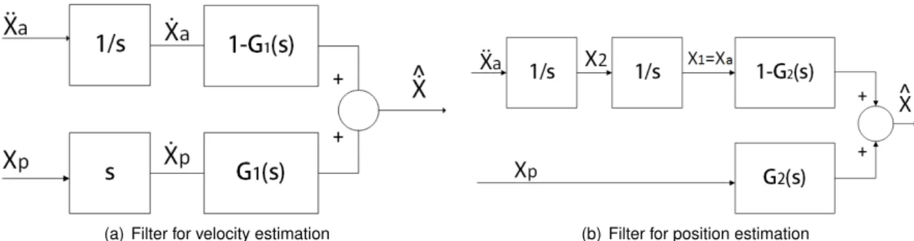
measurements. For aircraft systems, the most common position source is the GPS, which is combined with the accelerometer measurements in the filter, which allow the estimation of both position and veloc-ity. An example of this is the following filter (Fig. 2.14).
(a) Filter for velocity estimation (b) Filter for position estimation
Figure 2.14: Inertial navigation complementary filter
Fig. 2.14 (a) represents the filter needed estimate velocity. ¨xais the linear acceleration measurement
coming from the accelerometer sensor while xp is the GPS position measurement. The integration 1s
attenuates the high-frequency noise in the acceleration measurement while s is a gain for the position measurement. As it is the velocity that is pretended to be estimated, it is required a second-order filter so that the transfer function allows attenuation at the high frequencies but also have a unity gain in low frequencies. The result is a second-order filter:
G1(s) = b s2+ as + b, (2.43) 1 − G1(s) = s2+ as s2+ as + b, (2.44)
where parameters a and b define natural frequency and damping factor for the filter. In the case of the position estimate - Fig. 2.14 (b) - , it is applied double integration to the acceleration measurement for obtaining a position and the GPS has unity gain. Another second-order transfer function is required:
G2(s) = as + b s2+ as + b, (2.45) 1 − G2(s) = s2 s2+ as + b, (2.46)