Comparison of organic matter decomposition between natural and artificial ponds

UNIVERSIDADE DE ÉVORA

Escola de Ciência e Tecnologia

Departamento de Biologia

Comparison of organic matter

decomposition between natural and

artificial ponds.

Pedro Miguel Portela Faísca

Orientação: Doutor Miguel Matias

Mestrado em Biologia da Conservação

Dissertação

2

University of Évora

Master in Conservation Biology

Dissertation

“Comparison of organic matter

decomposition between natural and

artificial ponds”

Pedro Miguel Portela Faísca

3

Index

Environmental and biological sampling ... 20

Statistical analysis ... 25

Results ... 27

Decomposition in mesocosms and natural ponds... 27

Decomposition in the mesocosms among different locations and treatments ... 29

Decomposition and environmental variables in mesocosms ... 32

Decomposition and macroinvertebrates in mesocosms ... 35

Discussion ... 37

Mesocosms versus natural ponds ... 37

Differences among regions... 38

The role of macroinvertebrates ... 39

Limitations/Future directions ... 41 Conclusion... 43 Acknowledgements ... 44 References ... 45 Appendix 1 ... 55 Appendix 2 ... 56 Appendix 3 ... 61 Appendix 4 ... 62

4

Figure Index

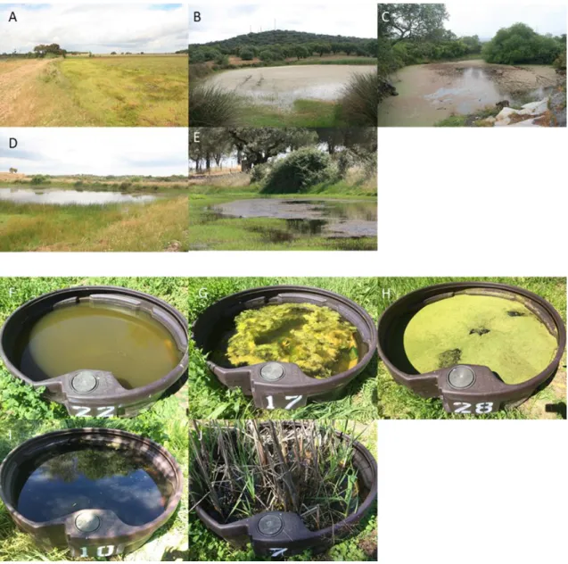
Figure 1- Aquatic systems used in the experiment. A-E) natural ponds; F-J) mesocosms ... 14

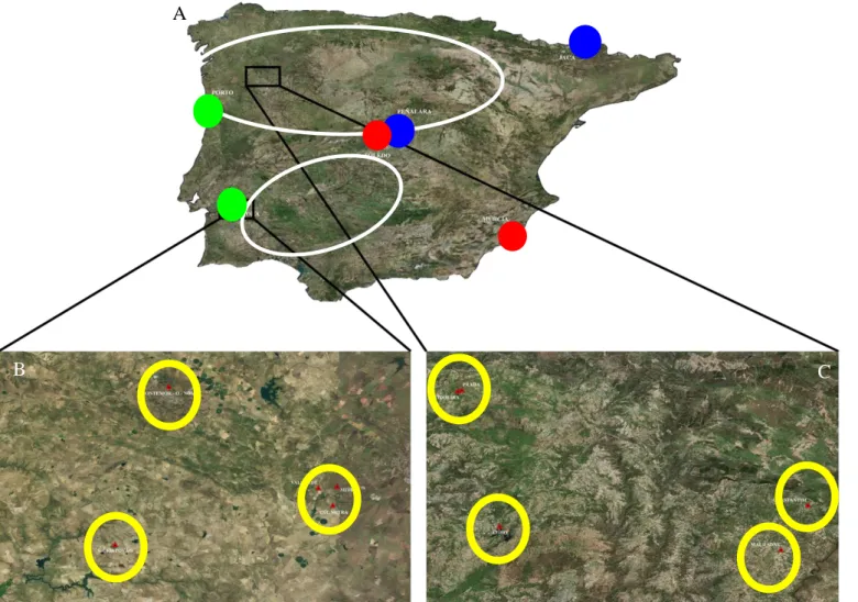
Figure 2- Map of the study area. A) Locations of the mesocosms in the Iberian Peninsula; red circles represent arid locations (Murcia and Toledo), green circles represent temperate locations (Évora and Porto) and blue circles represent mountain locations (Jaca and Peñalara); white circles represent Douro and Guadiana basins. B) Locations of the natural ponds in the Guadiana basin; red triangles and yellow circles represent the location of the natural ponds. C) Locations of the natural ponds in Douro basin; red triangles and yellow circles represent the location of the natural ponds. ... 15

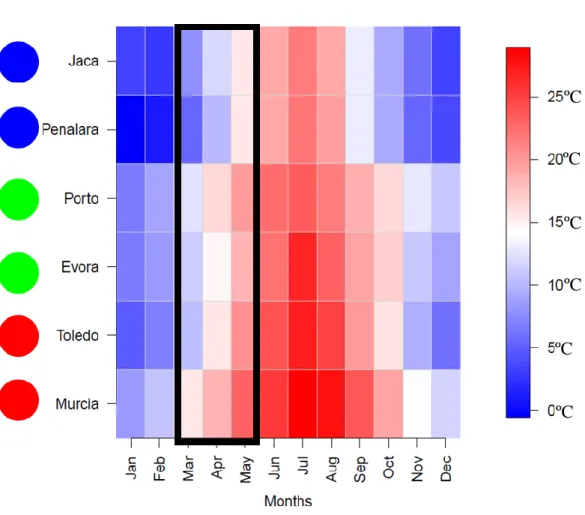
Figure 3- Monthly mean water temperature of the mesocosm through the year of 2015. ... 17

Figure 4- Net bags used in the decomposition experiment. A) Fine mesh bag (FN), which gives microbial decomposition (MD); B) Coarse mesh bag (CR), which gives total decomposition (TD); C) Controls; D) Experiment placed in mesocosms; and, E) Experiment placed in natural ponds. ... 19

Figure 5- Experimental design of the decomposition experiment. ... 19

Figure 6- Probe used to measure abiotic variables. ... 20

Figure 7- Core used for quantitative sampling in the mesocosms. ... 22

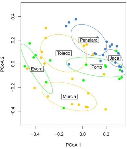
Figure 8-Principal coordinate analysis (PCoA) of the macroinvertebrate community of the mesocosms of each location ... 23

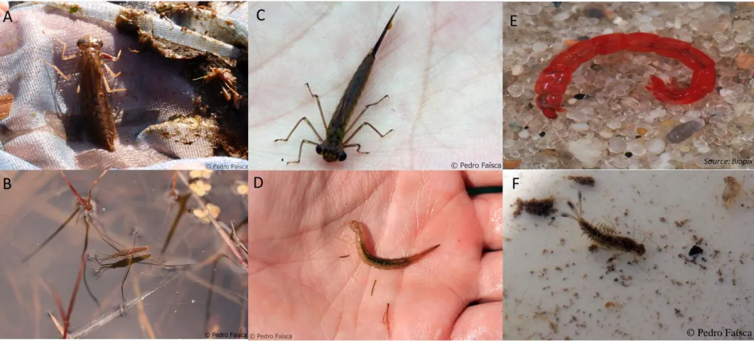
Figure 9- Major groups of macroinvertebrates present in the samples. A –Dragonfly (Anax sp.); B –Water strider (Gerris sp.); C –Damselfly (Zygoptera); D – Beetle larvae (Dytiscidae); E- Chironomid larvae (Chironomus sp.); F- Mayfly Larvae (Baetidae). ... 24

Figure 10- Relation between Mass loss (mg/day) and Tension loss (%). ... 25

Figure 11- Example of the ratio used in this study. If results were positive there is an effect of macroinvertebrates and if the results were negative, there is a positive effect of microorganisms. ... 26

Figure 12- Decomposition in the different systems. These plots are “box-plots” which are used to show variation in the samples. The bar represents the median and the two lines (or whiskers) indicate the spread of the data. In this plot we can see the mass loss (A) and tensile loss (B) of the cotton strips. These plots used the data from the controls of each of the systems. There are no differences between the systems. ... 27

Figure 13- Ratio between treatments in Mesocosms (Meso) and Natural Ponds (Natural) for Mass loss (A) and Tension loss (B). Both systems show a positive effect of macroinvertebrates for mass loss, while in tension loss natural ponds had a positive effect of microbial decomposition. See Methods section Statistical analysis for further details on the calculation of the ratio. ... 28

Figure 14- Mass Loss (A) and tension loss (B) of the cotton strips between treatment. TD had the highest mass loss and tension loss in both systems. ... 29

Figure 15- Decomposition across different location. These plots showed the mass loss (A) and tensile loss (B) of the cotton strips. These plots used the data from the controls of each of the locations separately. Évora was the location with the highest decomposition and Jaca was the location with less mass loss, while Porto was the location with less tension loss. ... 30

Figure 16- Ratio of the mass (A) and tensile loss (B) of the cotton strips between the two treatments. If the result was positive there is a positive effect of macroinvertebrates and if its negative it will mean a positive effect of microbial decomposition. ... 31

Figure 17- Mass Loss (A) and tension loss (B) of the cotton strips between treatment. These plots had data from the different treatments from each of the locations separately. TD had the highest mass loss and MD had the highest tension loss in Évora and Jaca. ... 32

Figure 18- Relation between accumulative daily temperature and mass loss in total decomposition (A) and microbial decomposition (B). ... 33

5

Figure 19- Relation between accumulative daily temperature and mass loss in total decomposition (A) and microbial

decomposition (B). ... 33

Figure 20- Relation between conductivity and mass loss in total decomposition (A) and microbial decomposition (B).

... 34

Figure 21- Relation between conductivity and Tension loss in total decomposition (A) and microbial decomposition

(B). ... 34 Figure 22- Relation between the abundance of gatherers and mass loss (A) and tension loss (B). ... 35

Appendix 1Figure 1-Relation between wet and dry weight (mg) of the cotton strips. There is a high correlation between both variables that allows for an estimation of the dry weight of the cotton strips using the formula Y = 0,982*X+(-0,00778)... 55

Appendix 3Figure 1- Principal coordinate analysis (PCoA) of the macroinvertebrate community in of both systemsin

mesocosms (“Meso”) and natural ponds (“Natural”). Each symbol indicates a pond that was used in Évora and Porto for this experiment in both systems adding to a total of 10 ponds, 5 ponds per region. ………....61

6

Table Index

Table 1- One-way ANOVA between systems and mass loss (mg/day) (A) and tension loss (%) (B). The differences between systems were not significant in both cases (p-value > 0.05). ... 27 Table 2- ANOVA with pond number as a random factor, between system and treatment for mass loss (mg/day) (A) and tension loss (%) (B). There were no significant differences for mass loss (p-value > 0.05), while in tension loss the differences between treatments was significant. * indicates significative differences at p-value < 0.05. ... 29 Table 3. One-way ANOVA between locations and mass loss (mg/day) (A) and tension loss (%) (B). In both cases the differences between location were significant (p-value < 0.05). *- significative variable ... 30 Table 4- ANOVA with mesocosm number as a random factor, between location and treatment for mass loss (mg/day) (A) and tension loss (%) (B). Mass loss only had significant differences in locations, while tension loss had significant differences in location, treatments and both interact (p-value < 0.05). *- significative variable ... 32 Table 5- Abundance of Functional Feeding groups in the ponds used for this experiment in all locations. ... 36 Appendix 2 table 1- Functional feeding groups of macroinvertebrate species found in the mesocosms. aff- Active filter feeders; gat- Gatherers/Collectors; gra- Grazers; pff- Passive filter feeders; pre- Predators; shr- Shredders. ... 56 Appendix 3 table 1-Anova between both systems and macroinvertebrate comunities ... 61 Appendix 4table 1- Abundance of macroinvertebrate species found in the five mesocoms used in the decomposition experiment in each location. ... 62

7

Comparison of organic matter decomposition between natural and

artificial ponds

Abstract

Litter decomposition is a key ecosystem service within aquatic ecosystems and is a complex process that is sensitive to environmental factors. The role of microbial and macrofaunal decomposers, and how it changes across environmental gradients is not yet fully understood. Decomposition was assessed across 6 biogeographical regions to determine the role of macroinvertebrates in this ecosystem service. Decomposition was estimated using standardized cotton strips, which were deployed in the mesocosms of each region. The role of macroinvertebrates was tested with an exclusion experiment which allowed or prevented the access of macroinvertebrates to cotton strips, a similar experiment was also conducted in natural ponds. After 64 days the cotton strips were collected, and mass loss and tensile strength were measured. There were significant differences in the rate of decomposition across different regions and no differences were found between systems. Macroinvertebrates played an important role, with gatherers being major players.

8

Comparação de decomposição de matéria orgânica entre charcos

naturais e artificiais

Resumo

A decomposição é um serviço de ecossistema chave e um processo complexo sensível a factores ambientais. O papel de decompositores microbianos e da macrofauna, e como este papel muda num gradiente ambiental não é completamente entendido. A decomposição foi avaliada em 6 zonas biogeográficas para determinar o papel de macroinvertebrados neste serviço de ecossistema. A decomposição foi estimada utilizando tiras de algodão, colocadas em mesocosmos nas diferentes regiões. O papel dos macroinvertebrados foi testado através de uma experiência de exclusão que permitia ou impedia o acesso de macroinvertebrados às tiras, uma experiência semelhante foi realizada em charcos naturais. Ao fim de 64 dias, as tiras de algodão foram recolhidas e a perda de massa e tensão foram quantificadas. Encontraram-se diferenças significativas na decomposição entre as diferentes regiões, mas não se observaram diferenças entre sistemas. Os macroinvertebrados têm um papel importante neste serviço de ecossistema, sendo as espécies colectoras as mais importantes.

9

Introduction

Freshwater ecosystems are a major component of biodiversity and may be one of the most threatened ecosystems in the world (Szöllosi-Nagy et al., 1998; Saunders et al., 2002; Dudgeon et al., 2005; Higgins et al., 2005). Declines in biodiversity, which includes the variety of living organisms, genetic differences among them, communities and ecosystems in which they occur, and the ecological and evolutionary processes that keep them functioning (Noss & Cooperrider, 1994; Delong, 1996), are far greater in freshwater than in terrestrial ecosystems (Frissell et al., 1996; Sala et al., 2000). It is estimated that future extinction rates in freshwater ecosystems will be five times greater than that of terrestrial ecosystems, and three times greater than that of coastal marine ecosystems (Ricciardi et al., 1999; Saunders et al., 2002). The threats to global freshwater biodiversity can be grouped under five interacting categories: over exploitation; water pollution; flow modification; destruction or degradation of habitat; and, invasion by exotic species (Brönmark & Hansson, 2002; Saunders et al., 2002; De Meester et al., 2005; Dudgeon et al., 2005; Oertli et al., 2005; Declerck et al., 2006; Céréghino et al., 2007). The combined and interacting influences of the five major threat categories have resulted in population declines and range reduction of freshwater biodiversity worldwide (Dudgeon et al., 2005).

Recent studies have explored the links between biodiversity and ecosystem function (Hooper et al., 2005; McIntyre et al., 2007; Vaughn et al., 2007; Strayer et al., 2010). Ecosystem functions depend on species richness and composition, but the size and nature of this effect depend on the species being gained or lost, the ecological process under consideration, and the characteristics of the ecosystem (Strayer et al., 2010). In these key ecosystem functions there are landscape related functions (e.g., migration corridors and stepping stones; De Meester et al., 2005), leaf litter decomposition that plays an essential role in controlling the carbon and nutrient cycles (e.g., Kampfraath et al., 2012; Vysná et

al., 2014;) and primary production (e.g., Dang et al., 2009).

Determining the ecological condition of ecosystems is a key challenge for effective resource management (Tiegs et al., 2013). Traditional assessment has focused entirely on ecosystem structure (e.g., invertebrate community composition, water quality), and neglected ecosystem processes (e.g., primary production, organic-matter decomposition; Fritz et al., 2011; Niyogi et al., 2013; Tiegs et al., 2013; Vysná et al., 2014). Nevertheless, several studies have drawn attention that using only a structural organization of biota, as

10 indicators of ecosystem health (without considering also its functional role) contribute little to ecosystem functioning and therefore should not be used as the only indicator in assessment of the ecological status of the water bodies (Bunn and Davis, 2000). As a response to these issues, the 5th European Water Framework Directive (WFD - Directive 2000/60/CE) requires additional incorporation of the ecosystem processes in stream assessment protocols. Recently, functional measures have received considerable attention due to their sensitivity in response to environmental change (Bunn et al. 1999; Fellows et

al. 2006; Young et al. 2008). One of the most conspicuous descriptors of the

ecosystem-level processes is the measure of organic matter processing (e.g. litter breakdown, generation and export of fine-particulate organic matter, secondary production of macroinvertebrates (Gessner & Chauvet, 2002)) have been proposed as indices of ecosystem function that may add to the structural measures (Gessner & Chauvet, 2002; Young et al., 2008; Silva-Junior et al., 2014; Piggot et al., 2015).

Ponds are small (1 m2 _{to about 5 ha), man-made or natural shallow waterbodies which}

maintain water level permanently or temporarily (De Meester et al., 2005; Céréghino et

al., 2007). Due to their small size and the ability to easily be manipulated experimentally,

ponds represent an ideal model for controlled studies of many basic ecosystem processes (e.g., primary production, organic matter decomposition; De Meester et al., 2005; Céréghino et al., 2007), and might function as an early warning system for long term effects on larger aquatic systems (Céréghino et al., 2007). Aquatic ecosystems have dramatically decreased during the last century (Saunders et al., 2002; Oertli et al., 2005; Le Viol et al.,2009), between 1984 and 2015 permanent surface water has disappeared from an area of almost 90.000 Km2 (Pekel et al., 2016). Ponds were found to be the most species rich aquatic habitat (Davies et al., 2008), and, like natural ponds, man-made ponds support wildlife and may function as corridors and refuges for the native fauna and flora (Le Viol et al., 2009). Although artificial ponds differ in abiotic conditions from surrounding ponds, they support communities of aquatic invertebrates as rich and as diverse at the family level as natural ponds and may contribute to reinforcing the pond network and consequently the abundance of such habitats on a regional scale (Le Viol et

al., 2009).

Temporary ponds are fluctuating waterbodies with recurrent seasonal phases of flooding and desiccation in most years. Although some macroinvertebrates persist in ephemeral habitats as resting stages in dry sediment, dispersal to more permanent waterbodies are

11 the main strategy through which they survive dry phases in temporary aquatic habitats (Florencio et al., 2011). Temporary ponds support relatively fewer aquatic macroinvertebrates when compared to more permanent sites, being the species richness related to the length of the flooded period (Pyrovetsi & Papastergiadou, 1992; Collinson

et al., 1995). However, there is no evidence of temporary ponds being species-poor

(Collinson et al., 1995; Williams et al., 2004; Oertli et al., 2005), in fact shallow ponds can dry out to only mud and produce no effect on species richness, species rarity or community composition in the following year, might serve as proof (Collinson et al., 1995; Céréghino et al., 2007; Sayer et al., 2012). Temporary ponds have very distinctive macroinvertebrate communities (De Meester et al., 2005; Céréghino et al., 2007), because periodicity of water confers specific advantages to particular species, including an absence of fish predation, nutritionally rich substrates and warm spring temperatures (Collinson et al., 1995; De Meester et al., 2005). The same conclusion was reached by Fairchild et al. (2003), in a study focused on beetle communities in temporary and permanent ponds. The author concluded that the hydroperiod together with other environmental variables has strong effect on community composition and distribution of beetles.

Organic matter decomposition is one of the most important ecosystem processes and is essential to the trophic dynamics of freshwater ecosystems (Boyero et al., 2011; Handa

et al., 2014; Piggott et al., 2015), where the decomposition of cellulose is a central part

of carbon and nutrient cycles and energy transfer within the ecosystem (Goodman et al., 2010). Decomposition processes are a complex group of physical, chemical, animal and microbial interactions (Webster & Benfield, 1986; Allan & Castillo, 2007; Piggott et al., 2015; Santonja et al., 2017) that are thought to be sensitive to climate warming (Boyero

et al., 2011; Piggott et al., 2015). Also, organic matter decomposition varies locally as a

function of environmental factors (e.g., temperature and nutrients) and substrate quality (Webster and Benfield, 1986; Costantini et al., 2009; Goodman et al., 2010; Vysná et al., 2014; Martínez et al., 2015; Santonja et al., 2017). For example, higher temperatures and high nutrient availability can increase microbial decomposition, while an increase of fine sediments can decrease decomposition by reduction of macroinvertebrates’ and microbial activity (Young et al., 2008; Goodman et al., 2010; Vysná et al., 2014). In quantitative terms, shredder macroinvertebrates have a crucial role in decomposition (Cummins & Klug, 1979; Handa et al., 2014; Garcia-Palacios et al., 2016; Santonja et al., 2017). They

12 have a direct and indirect contribution to litter decomposition by consuming and fragmenting litter material (Graça, 2001; Santonja et al., 2017); which provides additional nutrients and habitats for microbes and creates new resources for other organisms (collectors and filter-feeding invertebrates) in the aquatic food web, through the production of fine particulate organic matter (Joyce & Wotton, 2008; Santonja et al., 2017).

Litter-bag experiment for quantifying litter decomposition, is the most common process to assess stream-ecosystem functioning (Young et al., 2008; Fritz et al., 2011; Niyogi et

al., 2013; Tiegs et al., 2013; Vysná et al., 2014; Ferreira & Guérold, 2017). However,

standardizing litter quality is a very challenging process (Tiegs et al., 2013). For example, litter quality (e.g., concentrations of nutrients, secondary compounds) varies widely among species in ways that influence decomposition (Petersen & Cummins, 1974; Webster & Benfield, 1986; Newman et al., 2001; Goodman et al., 2010; Tiegs et al., 2013; Vysná et al., 2014; Piggott et al., 2015; Ferreira & Guérold, 2017; Santonja et al., 2017). A very simple solution would be to use a single plant species to control for among species variation in assessment procedures (Boyero et al., 2011; Kampfraath et al., 2012; Tiegs et al., 2013). However, within species variation in litter quality that exists among regions, genetic differences among individual trees and other sources of variation, for example if a tree has been exposed to herbivory, complicate this solution (Tiegs et al., 2013). All the shortcomings of the litter-bag experiment can be overcome with the cotton-strip experiment (Boulton & Quinn, 2000; Clapcott & Barmuta, 2010; Goodman et al., 2010; Fritz et al., 2011; Niyogi et al., 2013; Tiegs et al., 2013; Vysná et al., 2014; Piggott

et al., 2015).

The cotton-strip experiment was first developed by the textile industry as a test to evaluate the effectiveness of fungicide treatment. Eventually it became used as a standard method for decomposition studies in soil and has recently been adapted to aquatic habitats (Latter & Walton, 1988). Being 95% cellulose, cotton-strips offer numerous advantages (Boulton & Quinn, 2000; Tiegs et al., 2013): (1) allow a degree of standardization of the material that is not possible with plant litter; (2) cellulose is a highly ecological relevant compound because it constitutes the bulk of plant litter (Kampfraath et al., 2012; Tiegs et al., 2013); (3) less expensive and time consuming, cotton fabric is inexpensive and loss of tensile strength typically occurs faster than litter-mass loss, requiring smaller incubation times (Boulton & Quinn, 2000; Niyogi et al., 2013; Tiegs et al., 2013); (4) provide a suitable

13 substrate for leaf-colonizing fungi and bacteria and can serve as a food source for some leaf-shredding invertebrates (Tiegs et al.,2007). Although, decomposition of cotton strips might offer advantages in terms of standardization, it is primarily a measure of microbial enzymes to decay cellulose and is not a perfect surrogate for leaf decomposition, because materials using natural cotton have an uncertain and variable chemical composition and is extremely simple when compared to natural plant litter. (Tiegs et al., 2007; Kampfraath

et al., 2012; Vysná et al., 2014; Piggot et al., 2015). And, despite its economic and

logistical ease, few studies have used the cotton strip experiment as way of assessing ecosystem function on aquatic ecosystems (Young et al., 2008; Goodman et al., 2010). We are using this method because we needed a material that would be economical, easy to transport and that could be deployed in all the locations in this way we would have a standard origin for the organic matter that would allow us to compare different regions without focusing on the difference in leaves.

The threats that small ponds are faced with opens the possibility to use experimental systems, like mesocosms, to test how changes in environmental variables might affect ecosystem function in a natural system. With that in mind, one of the main objectives of this study was to compare decomposition between natural ponds and mesocosms. Diversity is linked to the function of the ecosystem, therefore the decline in worldwide biodiversity might cause changes in ecosystem function (e.g. organic matter decomposition). It’s crucial to understand the exact role of freshwater macroinvertebrates on one of the most important ecosystem functions (organic matter decomposition) to help predict how changes in biodiversity will affect the function of these ecosystems. For this reason, another objective of this study is to understand if and how macroinvertebrates contribute to organic matter processing. To meet this objective macroinvertebrate structure and organic matter decomposition was compared between freshwater mesocosms and natural ponds across 6 different locations. The hypotheses of this study is that there are no differences in decomposition rates between natural ponds and mesocosms, decomposition differs across different locations and macroinvertebrates play an important role in organic matter decomposition.

14

Methods

Study Area

The main objective of this study is to compare decomposition of organic-matter between natural ponds (Figure 1 A-E) and aquatic mesocosm (experimental enclosures that vary from one to thousands of litters and can test community and ecosystem-level responses to change (Stewart et al., 2013); Figure 1 F-J). In this study we also made a comparison between six regions (Évora, Porto, Murcia, Toledo, Peñalara and Jaca; Figure 2) using mesocosms and tested the role of macroinvertebrates in this ecosystem service. Litter-bags are easy to implement, cost-effective, reliable and accurately reflect the ecosystems condition (Fritz et al., 2011; Kampfraath et al., 2012; Tiegs et al., 2013).

Figure 2- Map of the study area. A) Locations of the mesocosms in the Iberian Peninsula; red circles represent arid locations (Murcia and Toledo), green circles represent

temperate locations (Évora and Porto) and blue circles represent mountain locations (Jaca and Peñalara); white circles represent Douro and Guadiana basins. B) Locations of the natural ponds in the Guadiana basin; red triangles and yellow circles represent the location of the natural ponds. C) Locations of the natural ponds in Douro basin; red triangles and yellow circles represent the location of the natural ponds.

A

These locations have very distinct climates (Figure 3). The climate in Murcia is Mediterranean with semi-arid features, with an average annual temperature between 15.0 ºC and 19.0 ºC and short winters and long and hot summers. The annual rainfall is less than 350 mm, except for some areas in the upper northwestern lands where it exceeds 600 mm, rainfall distribution is irregular with long dry periods combined with short and intense rainfall events (Alonso-Sarría et al., 2016). Toledo has a continental semiarid climate with an annual rainfall of 487 mm and an average annual temperature of 14.0 ºC (Hernández et al., 2007). The climate in Évora is typically Mediterranean, with a hot and dry summer. More than 80% of annual precipitation occurs between October and April. The long-term mean annual temperature is 15.0-16.0 ºC and average annual precipitation of 669 mm (Pereira et al., 2007). The most significant feature of the Porto climate is the annual rainfall level (1236 mm) and its irregular distribution throughout the year, mainly concentrated in winter and spring. Due to the maritime influence Porto has mild temperatures with an annual mean of 14.4 ºC. No cold season can be found in Porto, being January the coldest month, with an average of 9.3 ºC. The mean summer temperature is about 18.1 ºC, although between May and September, very high temperatures can be reached (Abreu et al., 2003). In Jaca, climate conditions are typically alpine, with cold mean annual temperatures that ranged between -0.7 ºC and 5.0 ºC and high-mean annual precipitation values well distributed along the year (Garcia-Pausas et al., 2007). In Peñalara, the mean annual temperature is 6.3 ºC, with the coldest months being between December and April and hottest months being July and August. Annual precipitation is 1357 mm, the wettest months are between October and May and the driest being between July and August, with higher precipitation being in late autumn and early winter (Palacios

et al., 2003).

The Douro basin, which is located across the northern-central Iberian Peninsula, is characterized by having a temperate climate with some continental and Mediterranean influences, this is evident by the annual precipitation values that vary within the region from 3000 mm in the upper Minho mountain tops, to 400 mm in the upper Douro valley, and the severe summer drought that are felt in the region (Asensi et al., 2011; Reis et al., 2014). The Guadiana river basin is enclosed in the Mediterranean region with semi-arid and sub-humid conditions (Valverde et al., 2015), it has a typical Mediterranean hydrological regime in which more than 80% of rainfall occurs between October and March (Collares-Pereira et al., 2000).

17 The mesocosms consist of small circular plastic tanks (160x60cm; 1000 L) that mimic small ponds. Each location has 32 mesocosms that were installed in 2014 and were initiated by adding 100 kg of topsoil collected locally and filled with local water. After the addition of water, the mesocosms were left to settle without further manipulation for a month, to allow the establishment of primary producers and insects. Following this initial settling period, mesocosms were inoculated with water collected from local natural and artificial ponds within a few kilometers from the experimental site. Finally, the mesocosms were inoculated with macroinvertebrates, macrophytes and sediment samples, adding a range of larger organisms. This sequential inoculation minimized potential differences among the sites associated with starting date, but also allowed to simulate a natural process of colonization in natural ponds. The natural ponds (Figure 1) used in this study ranged from farmland ponds to dams. All the habitats used were naturalized.

Figure 3- Monthly mean water temperature of the mesocosm through the year of 2015.

ºC ºC ºC ºC ºC ºC

18 Decomposition experiment

The decomposition experiment was done using cotton-strips (8x 2,5 cm) as surrogates for leaf-litter, following Tiegs et al. (2013). To test the role of macroinvertebrates in the decomposition of organic-matter, net bags with two different mesh-sizes were used, following previous studies (e.g., Tiegs et al., 2007; Raposeiro et al., 2014. Coarse net bags (CR; with a mesh size of 5 mm) were used to allow macroinvertebrates to access the cotton-strips, which gives total decomposition (TD). Fine net bags (FN; with a mesh size of 0.1 mm) were used to prevent macroinvertebrates to access the cotton-strips, which gives microbial decomposition (MD).

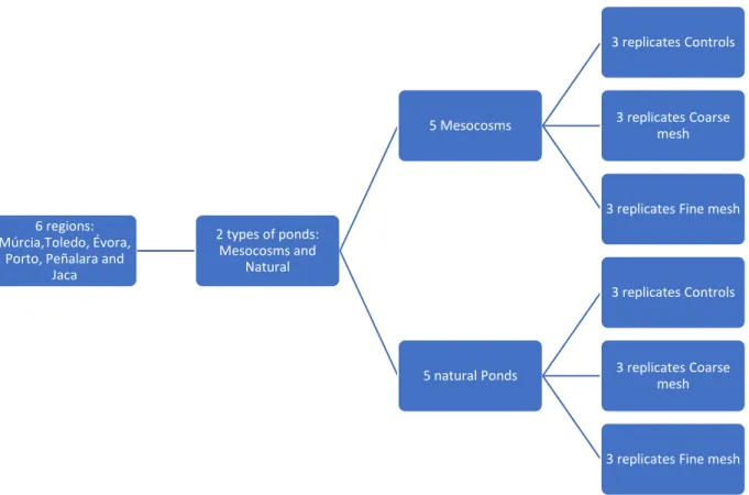
In each site, five mesocosms were selected for this experiment, the selection was done to have all dominant states represented (e.g., dominated by macrophytes, microalgae or animals), due to the high diversity of habitats that can be found between mesocosms within a location. In each mesocosm three treatments were implemented (Figure 4: A- FN; B- CR; C- Controls) with three replicates (Figure 5) each placed near the center of the pond (Figure 4 D).

Five natural ponds with longer flooded period were selected in each river basin. Here, cotton strips were placed in different types of habitat. In each pond the same three treatments were implemented (Figure 4: A- FN; B- CR; C- Controls) with seven replicates each (Figure 4 E) to ensure that at least three were retrieved.

The cotton strips were wet weighted before the experiment (T1), it was found that dry weight and wet weight were correlated (Appendix 1 Figure 1), so it was possible to estimate the dry weight of the cotton strips before the experiment using the formula, Y = 0,982*X+(-0,00778), and retrieved after 64 days. The cotton strips were cleaned using 80% ethanol to avoid the growth of fungi and microorganisms, and to wash sediment and algae build up. In the laboratory, they were dried at 38°C for 24 hours (Tiegs et al., 2013), and weighed to obtain the total mass loss (T2). Tensile strength was measured using a tensiometer (Hounsfield Test Equipment model H5KT-0088). Before the cotton strips were placed in the grips they were measured to see if they had the minimum length (4 cm) required to conduct the test and were marked at approximately 1 cm from the edges, they were placed in the grips in a way that they didn’t slipped or ripped in the points of contact. The tensiometer pulled at a rate of 2 cm/min. After the test the cotton strips were stored again.

19

6 regions: Múrcia,Toledo, Évora,

Porto, Peñalara and Jaca 2 types of ponds: Mesocosms and Natural 5 Mesocosms 3 replicates Controls 3 replicates Coarse mesh

3 replicates Fine mesh

5 natural Ponds

3 replicates Controls

3 replicates Coarse mesh

3 replicates Fine mesh

Figure 5- Experimental design of the decomposition experiment.

Figure 4- Net bags used in the decomposition experiment. A) Fine mesh bag (FN), which gives microbial

decomposition (MD); B) Coarse mesh bag (CR), which gives total decomposition (TD); C) Controls; D) Experiment placed in mesocosms; and, E) Experiment placed in natural ponds.

A

B

C

D

20 Environmental and biological sampling

The abiotic variables were measured using a HQ40D probe (Hach; Figure 6). The variables measured were pH, water temperature (ºC), conductivity (µS/cm) and dissolved oxygen (mg/L). In the case of the mesocosms, the oxygen measurements were done over two days at sunrise, midday and sunset to get an idea of the gross primary productivity and net primary productivity. Water temperature was measured continually in intervals of 30 minutes in 5 different mesocosms in each site using TidbitV2 HOBO data loggers (Onset). Detailed description of the physical and chemical characteristics of the mesocosms used in this study (Table 1).

Table 1- Physical and chemical characteristics of the studied mesocosms (mean values and standard deviation from the year 2017)

Location

Variables Múrcia Toledo Évora Porto Peñalara Jaca

Temperature (°C) 19.04 ± 2.68 18.92 ± 3.38 17.64 ± 3.03 18.2 ± 1.95 17.48 ± 2.62 17.11 ± 3.08 pH 9.97 ± 0.20 10.57 ± 0.15 9.74 ± 0.40 8.13 ± 0.76 9.13 ± 0.76 9.55 ± 0.85 Conductivity (µS/cm) 7775.63 ± 1389.45 1760.00 ± 259.23 598.50 ± 94.56 90.40 ± 17.29 102.26 ± 16.59 111.63 ± 29.61 chlorophyll a (µg/L) 34.21 ± 30.43 154.44 ± 168.42 45.45 ± 30.26 70.52 ± 97.87 71.40 ± 79.60 21.08 ± 1.76 Turbidity (NTU ) 0.006 ± 0.004 0.02 ± 0.03 2.60 ± 2.91 7.19 ± 4.29 0.01 ± 0.02 0.003 ± 0.002 Dissolved oxigen(mg/L) 4.97 ± 3.34 5.32 ± 2.12 5.09 ± 3.48 8.43 ± 2.74 11.99 ± 3.92 10.17 ± 1.33

The macroinvertebrates sampling in mesocosms consisted in a quantitative. For the quantitative sample, a core (50 L) was used (Figure 7), which represents 5% of the volume of the mesocosm. Ten swipes were done with aquarium net (mesh size of 500 µm) along the water column and sediment surface. All the matter that was scooped (e.g., organisms, organic-matter, sediment) was sieved through a 500 µm sieve and conserved in 96% ethanol.

Figure 7- Core used for quantitative sampling in the mesocosms.

In the natural ponds a D-frame net (mesh size of 250 µm) was passed 15 times considering the proportion of different micro-habitats found in the pond. The samples were conserved in ethanol at 96%.

In the laboratory, all samples were washed, and macroinvertebrates were sorted and then identified and counted under a dissecting microscope (SZX7 Olympus). In some cases, samples were subsampled using an 8x8 grid, and then sorted as many squares as possible in 2 hours. All macroinvertebrates were identified to the lowest taxonomic level possible using Tachet et. al 2010 (see Apendix 4 Table 1 and Figure 8 for data on species composition in all of the locations). In other cases, we used group specific ID keys to reach the species level (Figure 9 A and C) Odonata: Cham, 2012; Askew, 2004; Brooks & Cham, 2014. F) Ephemeroptera: Sowa, 1975; Alba-Tercedor, 1997. E) Chironomids: Wilson & Ruse, 2005; Langton, 1984; Brooks at al., 2008; Andersen et al., 2013). After identifying all the species, a biological trait table was created (Appendix 2, Table 1) with the functional feeding group (FFG) of each species using the Freshwater Ecology database (https://www.freshwaterecology.info).

23

Figure 8-Principal coordinate analysis (PCoA) of the macroinvertebrate community of the mesocosms of

Figure 9- Major groups of macroinvertebrates present in the samples. A –Dragonfly (Anax sp.); B –Water strider (Gerris sp.); C –Damselfly (Zygoptera); D – Beetle larvae

(Dytiscidae); E- Chironomid larvae (Chironomus sp.); F- Mayfly Larvae (Baetidae).

Statistical analysis

For the analysis tensile strength and mass loss data was used, despite showing some correlation (Figure 10). However, tensile strength loss appears to be more sensitive to small differences than mass loss (Tiegs et al., 2007). The analysis was done using R version 3.4.2, to test the differences between locations an analysis of variance (one-way ANOVA) was used with ‘location’ and ‘tension loss’ or ‘mass loss’ as main factors. To test the difference between treatments we used linear mixed-effects models using the ‘lmer’ function in R package lme4 (Bates et al., 2015), with mesocosm number as a random factor, and two-way ANOVA with ‘location’, ‘treatment’ and ‘tension loss’ or mass loss’ as main factors. To test the differences between systems a one-way ANOVA was used with ‘system’ and ‘tension loss’ or ‘mass loss’ as main factors. Differences between treatments was tested using linear mixed-effects models using the function ‘lmer’ in R package lme4 (Bates et al., 2015), with pond number as a random factor, and two-way ANOVA with ‘system’, ‘treatment’ and ‘tension loss’ or ‘mass loss’ as main factors.

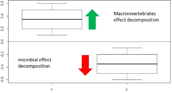
26 To assess the effect of macroinvertebrates in the tensile strength of the cotton strips a ratio was done using the formula: ln (TD/MD), where TD represents total decomposition, which is related with the coarse mesh bags, and MD represents microbial decomposition, which is related with the fine mesh bags. This ratio is similar to what other studies have done (Cardinale et al., 2006, Mayer-Pinto et al., 2016). If the result was positive there is a positive effect of macroinvertebrates and if its negative it will mean a positive effect of microbial decomposition (Figure 11).

Figure 11- Example of the ratio used in this study. If results were positive there is an effect of

macroinvertebrates and if the results were negative, there is a positive effect of microorganisms.

To check for differences in the macroinvertebrate community between natural ponds and mesocosms a principal coordinate analysis (PCoA) was done using the function ‘betadisper’ in R package vegan (Oksanen et al., 2018). To determine which environmental variables and macroinvertebrate’s feeding type best explained the decomposition in the mesocosms, a variable selection by Akaike information criterion (AIC) was used. Relevant variables were then plotted and tested to determine if there was a correlation using linear models

27

Results

Decomposition in mesocosms and natural ponds

There were no apparent differences between both systems in mass loss (A) and tension loss (B) between mesocosm (Meso) and natural ponds (Natural) using controls (Figure 12). Table 2 shows that there are no significant differences between systems for mass loss (A) and tension loss (B) (p-value > 0.05).

Figure 12- Decomposition in the different systems. These plots are “box-plots” which are used to show variation in the samples. The bar represents the median and the two lines (or whiskers) indicate the spread of the data. In this plot we can see the mass loss (A) and tensile loss (B) of the cotton strips. These plots used the data from the controls of each of the systems. There are no differences between the systems.

Table 2- One-way ANOVA between systems and mass loss (mg/day) (A) and tension loss (%) (B). The differences

between systems were not significant in both cases (p-value > 0.05).

A) Mass Loss

Df Sum Sq Mean Sq F value Pr(>F)

System 1 7e-7 6.51E-07 0.064 0.801

Residuals 55 5.61e-4 1.02E-05

B) Tension Loss

Df Sum Sq Mean Sq F value Pr(>F)

System 1 703 703.4 1.983 0.165

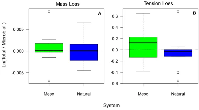
28 The ratio between treatments in Mesocosm (Meso) and Natural Ponds (Natural) for Mass loss (A) and Tension loss (B) showed that both systems showed a positive effect of macroinvertebrates for mass loss, while in tension loss natural ponds have a positive effect of microbial decomposition (Figure 13).

Figure 13- Ratio between treatments in Mesocosms (Meso) and Natural Ponds (Natural) for Mass loss (A)

and Tension loss (B). Both systems show a positive effect of macroinvertebrates for mass loss, while in tension loss natural ponds had a positive effect of microbial decomposition. See Methods section Statistical analysis for further details on the calculation of the ratio.

Mass loss (A) and tension loss (B) between the two treatments in Mesocosms (Meso) and Natural ponds (Natural) showed that TD had the highest mass loss and tension loss in both systems (Figure 14). The differences between system were not significant in both mass loss and tension loss (ANOVA: p-value > 0.05), while the differences in treatment where only significant for tension loss (ANOVA: p-value < 0.05) (Table 3). PCoA showed that in Natural Ponds there are no significant differences between both locations, while in the mesocosm there are differences between locations (Appendix 3, Figure 1; Table 1, p-value > 0.05).

29

Figure 14- Mass Loss (A) and tension loss (B) of the cotton strips between treatment. TD had the highest

mass loss and tension loss in both systems.

Table 3- ANOVA with pond number as a random factor, between system and treatment for mass loss

(mg/day) (A) and tension loss (%) (B). There were no significant differences for mass loss (p-value > 0.05), while in tension loss the differences between treatments was significant. * indicates significative differences at p-value < 0.05.

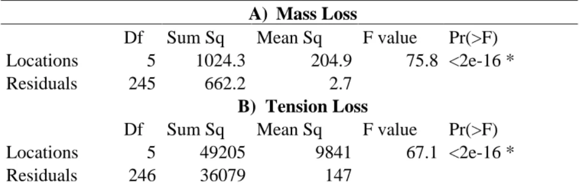
Decomposition in the mesocosms among different locations and treatments Decomposition was different across all locations (Figure 15). Évora was the location with the highest mass loss and tension loss (mean mass loss = 6.01 mg/day; mean tension loss = 95%), while Jaca had the lowest mass loss (mean mass loss = 0.018 mg/day) and Porto was the location with the lowest tension loss (mean tension loss= 51%). The differences between locations were significant (One-way ANOVA: p-value < 0.05) in both mass loss and tension loss (Table 4).

A) Mass Loss

Sum Sq Mean Sq NumDF DenDF F value Pr(>F)

System 2.56e-07 2.56e-07 1 14.878 0.0999 0.7564

Treatment 3.50e-06 1.75e-06 2 36.025 0.6825 0.5118

System:treatment 2.98e-06 1.49e-06 2 36.025 0.5816 0.5641 B) Tension Loss

Sum Sq Mean Sq NumDF DenDF F value Pr(>F)

System 80.89 80.89 1 14.739 0.6173 0.4445

Treatment 1031.07 515.54 2 36.005 3.9344 0.0285*

30

Figure 15- Decomposition across different location. These plots showed the mass loss (A) and tensile loss

(B) of the cotton strips. These plots used the data from the controls of each of the locations separately. Évora was the location with the highest decomposition and Jaca was the location with less mass loss, while Porto was the location with less tension loss.

Table 4. One-way ANOVA between locations and mass loss (mg/day) (A) and tension loss (%) (B). In

both cases the differences between location were significant (p-value < 0.05). *- significative variable.

A) Mass Loss

Df Sum Sq Mean Sq F value Pr(>F) Locations 5 1024.3 204.9 75.8 <2e-16 *

Residuals 245 662.2 2.7

B) Tension Loss

Df Sum Sq Mean Sq F value Pr(>F) Locations 5 49205 9841 67.1 <2e-16 *

31 The ratio between both treatments, Total decomposition (TD) and Microbial decomposition (MD), using mass loss and tension loss showed there was a very clear positive effect of macroinvertebrates in all locations when we use either mass loss or tension loss (Figure 16).

Figure 16- Ratio of the mass (A) and tensile loss (B) of the cotton strips between the two treatments. If the

result was positive there is a positive effect of macroinvertebrates and if its negative it will mean a positive effect of microbial decomposition.

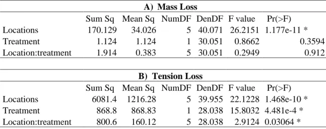
Mass loss (A) and tension loss (B) between the two different treatments in all locations showed that TD had the highest mass loss in all the locations (mean mass loss = 0.17 mg/day), while tension loss was higher for MD in Évora and Jaca (mean tension loss = 77 %) (Figure 17). For mass loss, only the differences between locations were significant (ANOVA: p-value < 0.05) while the differences between treatments were not significant (ANOVA: p-value > 0.05) with no interaction between both (ANOVA: p-value > 0.05; Table 4). For tension loss the differences between locations and treatments were significant with interaction between both (ANOVA: p-value < 0.05) (Table 4), but there were two exceptions to this interaction in Évora and Jaca with higher decomposition in MD.

32

Figure 17- Mass Loss (A) and tension loss (B) of the cotton strips between treatment. These plots had data

from the different treatments from each of the locations separately. TD had the highest mass loss and MD had the highest tension loss in Évora and Jaca.

Table 5- ANOVA with mesocosm number as a random factor, between location and treatment for mass

loss (mg/day) (A) and tension loss (%) (B). Mass loss only had significant differences in locations, while tension loss had significant differences in location, treatments and both interact (p-value < 0.05). *- significative variable.

A) Mass Loss

Sum Sq Mean Sq NumDF DenDF F value Pr(>F) Locations 170.129 34.026 5 40.071 26.2151 1.177e-11 *

Treatment 1.124 1.124 1 30.051 0.8662 0.3594

Location:treatment 1.914 0.383 5 30.051 0.2949 0.912 B) Tension Loss

Sum Sq Mean Sq NumDF DenDF F value Pr(>F) Locations 6081.4 1216.28 5 39.955 22.1228 1.468e-10 * Treatment 868.8 868.83 1 28.038 15.8032 4.481e-4 * Location:treatment 800.6 160.12 5 28.038 2.9124 0.03064 *

Decomposition and environmental variables in mesocosms

The variable selection procedure done using Akaike information criterion (AIC) showed that the variables that explained decomposition in both treatments were accumulative daily temperature (Tacc) and conductivity (Cond) for both mass loss and tension loss. The relation between Tacc and mass loss between TD (A) and MD (B) , the model showed a pattern for TD with higher mass loss in the intermediate values of Tacc (Figure 18A) TD: R2 = 0.16, p-value < 0.05), while in MD the model did not show a clear pattern (Figure 18B) MD: R2 = 0.12, p-value > 0.05). The relation between Tacc and tension loss

33 between TD (A) and MD (B), in both treatments, the model did not show any clear pattern (Figure 19A) TD: R2 = 0.02 p-value > 0.05; Figure 19B) MD: R2 = -4.1e-4 , p-value < 0.05).

Figure 18- Relation between accumulative daily temperature and mass loss in total decomposition (A) and

microbial decomposition (B).

Figure 19- Relation between accumulative daily temperature and mass loss in total decomposition (A) and

microbial decomposition (B).

In the relation between Cond and weight loss between TD (A) and MD (B), in both treatments, the model showed that there is more mass loss in the intermediate values of

34 Cond and less in the extremes (Figure 20A) TD: R2 = 0.19, p-value < 0.05; Figure 20B) MD: R2 = 0.19, p-value < 0.05). The relation between Cond and tension loss between TD (A) and MD (B), in TD the model showed that there is more tension loss in intermediate values of conductivity (Figure 21A) R2 = 0.22, p-value < 0.05). MD did not show a clear pattern between the 2 variables (Figure 21B) R2 = 0.09, p-value > 0.05).

Figure 20- Relation between conductivity and mass loss in total decomposition (A) and microbial

decomposition (B).

Figure 21- Relation between conductivity and Tension loss in total decomposition (A) and microbial

35 Decomposition and macroinvertebrates in mesocosms

The variable selection done by AIC showed that the variable that better explained variation in mass loss and tension loss was the abundance of gatherers (Figure 22). In most of the location’s gatherers where present with higher relative abundances than most of the other function feeding groups, where Toledo was the location with the highest abundance (74.27%. Table 6) and Porto was the location with the lowest gatherer abundance (2.10%. Table 6). For more detailed information on the abundance on each of the species found in the mesocosms check Appendix 4, Table 1.

In both cases, the model showed there is a linear relation between decomposition and abundance of gatherer species (Mass loss: R2 = 0.21, p-value < 0.05; Tension loss: R2 = 0.45, p-value < 0.05).

Table 6- Abundance of Functional Feeding groups in the mesocosms used for this experiment in all locations (Mean abundances and standard deviation).

Location

Múrcia Toledo Évora

Functional Feeding Groups Mean Abundance Abundance (%) Mean Abundance Abundance (%) Mean Abundance Abundance (%) Active filter feeders 21.45 ± 15.64 7.01 2.18 ± 4.61 0.23 7.18 ± 9.93 2.50 Gatherers/Collectors 167.00 ± 313.87 54.59 582.36 ± 1091.45 61.07 266.64 ± 326.82 92.70

Grazers 95.27 ± 118.14 31.14 16.45 ± 28.39 1.73 6.27 ± 12.32 2.18

Passive filter feeders 0.00 ± 0.00 0.00 0.00 ± 0.00 0.00 0.00 ± 0.00 0.00

Predators 11.36 ± 11.72 3.71 340.91 ± 433.10 35.75 6.91 ± 6.57 2.40

Shredders 10.82 ± 34.21 3.54 11.73 ± 18.12 1.23 0.64 ± 1.72 0.22

Porto Jaca Peñalara

Functional Feeding Groups Mean Abundance Abundance (%) Mean Abundance Abundance (%) Mean Abundance Abundance (%) Active filter feeders 0.00 ± 0.00 0.00 0.7 ± 1.00 2.94 3.3 ± 3.98 1.32 Gatherers/Collectors 53.40 ± 65.95 41.17 4.2 ± 5.10 17.65 160.90 ± 212.28 64.59

Grazers 34.20 ± 26.77 26.37 0.70 ± 1.55 2.94 3.4 ± 2.62 1.36

Passive filter feeders 0.00 ± 0.00 0.00 0.10 ± 0.30 0.42 0.00 ± 0.00 0.00

Predators 35.80 ± 18.36 27.60 12.50 ± 9.21 52.52 24.10 ± 17.37 9.67

Discussion

No significant differences were found between rates of decomposition in natural ponds and mesocosms, with both having similar decomposition rates. Decomposition varied between different biogeographical regions, with Évora being the region with the highest decomposition. It was also shown that macroinvertebrates play an important role in the decomposition of organic matter and that gatherer species were the major players in this ecosystem service, despite of the low abundance of species that are considered real decomposers (e.g. shredders). In this study it was hypothesized and demonstrated that decomposition would vary across different biogeographical regions, that macroinvertebrates are important in the decomposition of organic matter and that there were no differences between natural ponds and mesocosms.

Mesocosms versus natural ponds

In this study, there were no significant differences between the two aquatic systems used: mesocosms and natural ponds. Based on what has been shown by other experiments artificial ponds are not very different from natural ones, supporting the same biodiversity that natural system support, with small differences being found in environmental variables (Céréghino et al.,2008; Ruggiero et al.,2008; Le Viol et al., 2009). Mesocosms, experimental enclosures with a thousand litters, were used as artificial ponds in this study. Mesocosms can be used to test community and ecosystem-level responses to change (Stewart et al., 2013; for more detailed explanation on the mesocosm used in this experiment check Methods’ subsection Study area).

Several mesocosms experiments, used at this scale, showed that they can reproduce the key elements of community structure and ecosystem functioning of small pond ecosystems (Jones et al., 2002; McKee et al., 2003; Ventura et al., 2008; Yvon-Durocher

et al., 2010). In Yvon-Durocher et al. (2010), the main conclusion reached was that the

data provided by their mesocosms could serve as a good baseline for understanding the mechanisms that control the effects of temperature on the metabolic balance of ecosystems. Although caution is needed when extrapolating such data from mesocosms to natural systems due to the great complexity and diversity in biotic and abiotic factors that can be found influencing the dynamic of these ecosystems. Since the mesocosms used in this study were inoculated with soil from nearby ponds (see Methods’ subsection

38 Study area), it was expected that there wouldn’t be many differences between both systems.

Differences among regions

Decomposition rates differed between the standardized aquatic mesocosms across different locations. Previous studies have shown that warmer climates promote higher decomposition rates than colder climates (e.g. Young et al., 2008). Similar to other studies, temperature was found to be one of the main factors responsible for the different decomposition rates observed in this experiment (Webster and Benfield, 1986; Costantini

et al., 2009; Goodman et al., 2010; Vysná et al., 2014; Martínez et al., 2015; Santonja et al., 2017). High temperatures can promote an increase in microbial decomposition

(Young et al., 2008; Goodman et al., 2010; Vysná et al., 2014), and has also been known to affect diversity and community composition of macroinvertebrates (Burgmer et al., 2006) by effecting the physiological processes of species, which may impact timing of life history events and trophic interactions (Ward, 1992). Brucet et al. (2012) found a greater diversity and abundance in colder and temperate climates, with Diptera being the most abundant group.

Another important factor in this experiment was conductivity. There is no consensus on the effects of this environmental factor on this ecosystem service. While there are studies that showed that high levels of conductivity led to an increase in decomposition (Weston et al., 2006; Craft, 2007; Morrissey et al., 2014), there are others that showed a decrease in this function (Rejmánkoná & Houdková, 2006; Roache et al., 2006; Neubauer, 2012). Conductivity is found to be strongly dependent of temperature (Hayashi, 2004) and can be related to the nutrient availability in the water (Stevens et al., 1995), in this case we can see the same thing as Weston et al. (2006) and Craft (2007), where high conductivity increased decomposition. A possible explanation for this can be found in Morrissey et al. (2014) were it was concluded that, conductivity affected the composition of the microbial community, which, in conjugation with other abiotic factors, stimulated extracellular enzymes and increased the decomposition of organic matter. Conductivity might also have indirect effects on decomposition by effecting the distribution of microbial community and structure of macroinvertebrate communities (Young et al., 2008). As shown in Brucet et al. (2012), conductivity has a negative effect on macroinvertebrate

39 diversity and abundance although, some groups are not affected (e.g. Odonata; Polychaeta) and some have a high tolerance to high conductivity levels (e.g. Diptera). As mentioned above (method subsection Statistical analysis), the loss of tensile strength appears to be more sensitive to small differences than mass loss (Tiegs et al., 2007). This leads to, environmental variables explaining differences in decomposition at the regional scale, while at a local scale microbial community composition seem to explain differences in decomposition more evidently, at least for the case of mass loss. The possible explanation for this is that the microbiological community is more sensitive to small changes in the environmental variables, that would only be detected at a local level. This can lead to more efficient decomposers being benefited in one pond, which leads to an increase in their abundance, but be impaired in another, which can lead to the absence of this species, due to a difference in temperature or conductivity. For example, Dang et al. (2009) found that variations of 8ºC in temperature would benefit a species of decomposing fungi that is more efficient than the other microbiological decomposer, which lead to faster decomposition rates.

The role of macroinvertebrates

Significant differences were found between total decomposition (decomposition by microbial and macroinvertebrates communities; TD) and only microbial decomposition (MD), with TD showing higher levels of decomposition, which can be related to the importance that macroinvertebrates have in the decomposition process. Although cotton strips have been found to be a less palatable than leaf litter as a food resource (Tiegs et

al., 2013), cotton strip palatability will improve with colonization and conditioning by

the microbial community (Graça, 2002; Tiegs et al., 2013). Studies that used the litter bag experiment have shown different results, some studies showing that there were no significant differences between TD and MD, where others defended that the role of macroinvertebrates was neglectable (Stockley et al., 1998; Lamed, 2000; Benstead et al., 2009; MacKenzie et al., 2013; Raposeiro et al., 2014; Ferreira et al., 2016). While other experiments found higher levels of decomposition in TD (Imbert & Pozo, 1989; Howe & Suberkropp, 1994; Graça & Canhoto, 2006; Tiegs et al., 2007; Jacob et al., 2010), showing a higher importance of macroinvertebrates in the decomposition of organic matter.

40 It should be expected that in biogeographical regions with stronger environmental filters, higher temperatures in the south of Spain and colder temperatures in the mountain regions, MD should be more important, due to the stresses that are placed on the macroinvertebrate communities (Brucet et al., 2012). On the other hand, in temperate regions TD would be more important due to their high diversity in terms of macroinvertebrates. However, this was not observed, decomposition was higher in TD in almost all the regions with strong environmental filters and the temperate locations showed higher MD. Although temperate locations had the highest diversity of macroinvertebrates, not all of these species had a relevant role in the decomposition of organic matter.

The abundance of gatherer species of macroinvertebrates was a factor that influenced decomposition in this experiment, where higher abundances were related with higher decomposition rates. Some of the studies mentioned above (e.g. Raposeiro et al., 2014; Ferreira et al., 2016) stated that the reason why they found no difference between treatments might be related to the fact that there were no shredding macroinvertebrates present in the ecosystem. Which is similar to what was found in this experiment, where there were very low abundances of true shredders in the mesocosms. Other studies defend that in the absence of shredding macroinvertebrates, other species with different feeding types might take the role of shredders (Chergui & Patteo, 1991; Lock, 1993; Graça, 2001). In Chergui & Patteo (1991) it was shown that in the absence of trichopteran and plecopteran in a Morocco stream there was a higher shredding affect by the gastropods species Melanopsis praemorsa and Physa acuta. Other studies also showed that the abundance of shredding macroinvertebrate was as important as the abundance of gatherers (Alvarez et al., 2001), where it was found that species of the Chironomidae subfamily, which are mostly classified as gatherers, to be responsible for the decomposition of the organic matter. Similar to what was found by Abelho (2008), that consistently found a high abundance of Chironomidae subfamily when compared to the abundance of shredders. In Silveira et al. (2013) it was determined that the Chironomidae larvae species of Chironomus, Polypedilum, and Tanytarsus, which are all gatherer macroinvertebrates, were the major species involved in decomposition, with the

Chironomus species being more associated with the late stages of decomposition and the Tanytarsus species more associated with the beginning stages of decomposition.

41 Limitations/Future directions

Despite the valuable information generated by this study, we acknowledge that there is still room for some improvements and further experiments to be done to expand our understanding of decomposition across different systems and scales. One important limitation in this study is the narrow temporal window of observation through which decomposition was measured. An obvious improvement to this methodology would be the use of multiple time points (i.e. deploy additional cotton strips for different time periods) to obtain accurate decomposition rates like it is done in most of the studies (e.g. Tiegs et al., 2007; Ferreira et al., 2016), but a single time point is adequate if effort must be minimized (Young et al., 2008).

Another area that should be taken into account is that, while cotton strips have proven to be a good method to measure decomposition (Boulton & Quinn, 2000; Tiegs et al., 2007; Tiegs et al., 2013), it only serves as a proxy for decomposition of leaves, so a similar study should be conducted using leaves, that were picked from trees from a single location and air-dried before being placed in the field (Boulton & Boon, 1991; Young et al., 2008). Another solution for the fact that cotton strips have a simpler chemical composition when compared with leaves, could be to conduct a new experiment related to the chemical composition of litter used in this experiment. In this type of experiment a decomposition and consumption tablet (DECOTAB), which consists of a high concentration of cellulose powder embedded in an agar matrix (Kampfraath et al., 2012), could be used instead. This material allows for a manipulation of its chemical composition, which allows to test how macroinvertebrates react to the presence of pesticides, for example.

Environmental variables like conductivity, dissolved oxygen, pH, chlorophyll and turbidity were only measured at the start of the experiment, which may lead to errors due to changes in these variables during the time the experiment was being conducted. Most of the studies (e.g. Ferreira et al., 2016) measured environmental variables at the beginning and at the end of the experiment. Studies that used the litter bag experiment would collect the macroinvertebrates found inside the mesh bags, this way its possible to determine which species were inside the litter bags and determine their abundance (Silveira et al., 2013; Biasi et al., 2013; Leite-Rossi et al., 2015). This study might have done the same. In some of the locations used in this study there are external factors that need to be considered, for example locations with trees nearby had an increase in leaf

42 litter availability, which gives an increase in availability of organic matter in these mesocosm and may affect the decomposition process. In future studies, leaf fall should be quantified by placing a container or a net on top of the ponds and leaving it there for a fixed time to determine leaf fall rates (Boulton & Boon, 1991).

Multiple macroinvertebrate taxa undergo ontogenetic diet shifts (Merritt, et al., 2008; Rosi-Marshall et al., 2016). To determine which group of macroinvertebrates were important for the decomposition of organic matter functional feeding groups (FFG) were used. FFG’s are a classification based on the organism’s mode of feeding (Cummins, 1973) and not the actual food resources that are being consumed. Despite this fact, FFG classifications may help understand the form of food resources consumed but cannot be counted as a measure of the identity of the food resources consumed (Rosi-Marshall & Wallace, 2002; Rosi-Marshall et al., 2016). One way to overcome this would be to determine what each macroinvertebrate species is eating, this could be done by analysing gut-content (Cummins, 1973, Rosi-Marshall et al., 2016) or by doing something similar to Holgerson et al. (2016), who labelled the organic material with a known isotope marker and then used a stable isotope analysis to “follow” the isotope through the food web. Finally, when working in regions with different climates, which affect decomposition (Young et al., 2008), the thermal gradient must be considered. The team at CIBIO-UE will continue the experiment at the Iberian Ponds facilities where a warming experiment will be conducted in which some mesocosms will be warmed to assess the impacts of climate change in freshwater ecosystems, like other studies (Mckee et al., 2003; Liboriussen et al., 2004; Yvon-Durocher et al., 2010; Fey et al., 2015).

43

Conclusion

Freshwater ecosystems, which are the focus of this thesis, are amongst the most threatened ecosystems in the world (Szöllosi-Nagy et al., 1998; Saunders et al., 2002; Dudgeon et al., 2005; Higgins et al., 2005), having decreased dramatically during the last century (Saunders et al., 2002; Oertli et al., 2005; Le Viol et al.,2009). Addressing this challenge requires developing a better understanding how these ecosystems function. Declines in biodiversity have been estimated to be far greater in freshwater than in terrestrial ecosystems (Frissell et al., 1996; Sala et al., 2000), with the increase in extinction risks when compared to other systems (Ricciardi et al., 1999; Saunders et al., 2002) making them highly vulnerable. The results showing similarities in decomposition of organic matter between mesocosms and natural ponds present us with opportunities to use experimental systems to further investigate how natural ecosystems function. Furthermore, the fact that decomposition varied between regions, may reflect, not only, differences in the environmental variables (as shown in this thesis), but shed some light on potential consequences of major environmental threats (e.g. over exploitation; water pollution; flow modification; destruction or degradation of habitat; and, invasion by exotic species; De Meester et al., 2005; Dudgeon et al., 2005; Oertli et al., 2005; Declerck

et al., 2006; Céréghino et al., 2007). The role macroinvertebrates and how a group of

aquatic organisms can have such a key role in this crucial ecosystem service, reinforces the need for continued research on the function of species in the ecosystem and how the potential loss of those species (and their functions), might harm the essential processes needed to maintain and conserve natural ecosystem services.

44

Acknowledgements

Firstly, I would like to thank my supervisor Miguel Matias for all the guidance, help and advice during this whole process.

To the team at CIBIO-UE, specially to Cátia Lúcio Pereira, Katarzyna Sroczynska, Andreu Castillo-Escrivà and Dora Neto for all the help and all that they have taught me along the way.

To the FCT project TrophicResponse (PTDC/BIA-BIC/0352/2014) for supporting this Master thesis.

To the teachers from the master in Conservation Biology at the University of Évora for passing on their teachings and experiences.

To professor Carla Cruz, Luís Guilherme Sousa, Eliana Machado and Sónia Ferreira, for their help in selecting natural ponds and during the sampling of those same ponds. To Pedro Raposeiro for all the hints and tips regarding decomposition of organic matter in these systems.

To my friends and classmates, Cláudio João, Ana Costa, Pedro Ribeiro and Tiago Malaquias for helping me in the field work.

To professor António Candeias and the team at the José de Figueiredo lab in Lisbon, for the opportunity to use the equipment in their facilities.

Lastly, I would like to thank my family and friends for the support and all the interest in my work for these past 2 years.