Cross-Sectional Tail Risk
and Equity Premium Prediction
Pavlo Onyshchenko 152412037
ABSTRACT
Common predictors of U.S. equity market risk premium fail out-of-sample. We provide a new cross-sectional measure of stock market tail risk. This performs better than the historical risk premium and other commonly used predictors for short- and long-term horizons. The predictive power of cross-sectional tail risk is especially remarkable for one-month horizon forecast and during contractions. We show that under a mean-variance setting, there is an economic increase in the expected return by more than 100% in the short-term and more than 50% for longer horizons.
Supervisor Professor José Faias
Dissertation submitted in partial fulfillment of requirements for the degree of International MSc in Finance, at Universidade Católica Portuguesa, September 2014.
ii
Acknowledgements
First of all, I would like to thank my supervisor Professor José Faias for continuous support during and even before writing my thesis. The course of Empirical Finance and our further research work motivated me to take this challenging path which I will never regret. His efforts in solving numerous doubts and problems, giving useful advice and just being a great person are priceless. I would not be able to reach this stage without the knowledge and inspiration he gave me.
Secondly, I want to thank Católica Lisbon School of Business and Economics for providing access to databases, subscription to academic literature and 24-hour per day availability. Additionally I thank Instituto Superior Técnico for providing working space during the summer break in August.
Thirdly, I would like to express gratitude to my beloved family which made it possible to study and live in a great country of Portugal and friends that helped me to focus during the work and to relax in periods apart of it, namely Rui Ascenso, José Cravo, Maksym Mishyn, Alexei Panuyshkin, Rustam Shamuradov and many other great people.
iii
Table of Contents
1
Introduction ... 1
2
Tail Risk Estimation ... 4
3
Data ... 6
4
Equity Premium Prediction ... 12
4.1 Standard Methodology and Results ... 12
4.2 Imposing Theoretical Restrictions on Regressions ... 16
4.3 Combination of individual predictors ... 19
5
Predictive Power and Real Economy ... 24
6
Economic Interpretation of R
2... 27
7
Conclusions ... 29
iv
Index of Tables
Table 1. Descriptive statistics of predictors. ... 11
Table 2. The correlation matrix of predictors... 12
Table 3. In-sample results of equity premium prediction ... 14
Table 4. Out-of-sample results of equity premium prediction ... 16
Table 5. Out-of-Sample results after slope and forecast restrictions ... 17
Table 6. Correlation matrix of OOS equity premium forecasts ... 20
Table 7. Out-of-sample results of combining predictors ... 22
Table 8. Pairwise forecast encopassing test results ... 23
Table 9. The OOS results during different business cycle stages ... 25
Table 10. OOS results during different GDP growth periods ... 26
Index of Figures
Figure 1. The evolution of tail risk measures for U.S. market ... 7Figure 2. Tail risk and future returns ... 8
Figure 3. Out-of-Sample performance of one-month horizon predictions ... 18
1
1
Introduction
The predictability of stock returns has been a great debate in academic literature over the last decades. At the same time, studying the properties of extreme events and market crashes became more important in the lights recent economic crises and market bubbles. The academics attempt to set a link of such events both with firm-specific characteristics [Wang et al. (2009), Bali et al. (2011), Annaert et al. (2013)] and with market-wide factors. The latter is often related to the distribution of returns, namely to tail risk, properties of which can be beneficial while being applied to asset pricing and allocation, risk management, valuation of derivatives and returns prediction [Longin and Solnik (2001), Poon et al. (2004), Fousseni et al. (2014)]. Regarding the latter, the theory suggests that during the periods of increasing tail risk investors would demand higher equity premium. Together with this, the persistence of tail structure [Gardes and Stupfler (2013)[Jiang and Kelly (2014)] asserts that the implied return predictability is substantial.
This paper aims to predict the U.S. stock market excess returns using a new variable, the cross-sectional tail risk. It is estimated by applying Hill’s (1975) estimator to the daily cross-section of stock returns and averaging obtained tail exponents within a month. By doing this, we improve the cross-sectional and time series properties of alternative measures of tail risk. We evaluate the predictive power of various valuation ratios and macroeconomic variables used in the past literature over the last fifty years. We show that cross-sectional tail risk outperforms out-of-sample the historical average and all predictors. Ever since Bates and Granger (1969), the forecast combinations have been proven to be better predictors than individual forecasts by numerous authors.1 However, we show that the cross-sectional tail risk predictions beat the forecast
1
See Raftery et al. (1997), Stock and Watson (2004), Elliott and Timmermann (2005), Timmermann (2006), Mamaysky et al. (2007, 2008), Rapach et al. (2010), Elliott and Drive (2011), Elliott et al. (2013) and Hsiao and Wan (2014).
2
combinations. We test our results on one-month, three-month, one-year and three-year horizons. The superior predictive power of tail risk over alternative predictors is especially distinctive for short-horizon forecasts.
The first insights about the relation of valuation indicators and future returns are dated back to the studies of Dow (1920) and Graham and Dodd (1934) which affirm that high valuation ratios should be followed by high subsequent returns as they point out the undervalued stock. In support of this view, Campbell and Shiller (1988a, 1988b) and Fama and French (1988) assert potential predictability of stock returns over long horizons using valuation ratios. During the last several decades the academic literature both continued providing evidence of valuation ratios’ predictive power [Pontiff and Schall (1998), Kothari and Shanken (1997), Lewellen (2004)] and suggested other variables to predict subsequent returns, such as corporate issuing activity and payout policy [Lamont (1998), Baker and Wugler (2000) and Boudoukh et al. (2007)], variables related to corporate and government bond yields [Campbel (1987), Ang and Bekaert (2007)] and market volatility [Guo (2006)].
Although the literature about prediction of stock returns is extensive, the number of academic articles on out-of-sample (OOS) forecasts is far scarcer. One of such studies is conducted by Goyal and Welch (2008) who argue that the historical mean performs at least as well as other equity premium predictors out-of-sample. The authors show that positive performance of commonly studied predictors vanished with time or is attributed to the oil shock of 1973-74. The conclusions of Goyal and Welch (2008) have been widely opposed by more recent studies. Campbell and Thompson (2008) suggest that OOS results are significantly improved if theoretical constraints are imposed on predictive regressions. Lettau and Nieuwerburgh (2008) adjust price ratios to changes in economy state and document positive out-of-sample predictability using
3
adjusted ratios. Rapach et al. (2010) show that combinations outperform individual OOS forecasts and consistently yield positive R2. This happens because by reducing the estimation noise and incorporating useful information from different predictions, combinations better reflect broad macroeconomic conditions. Ferreira and Santa-Clara (2011) propose forecasting separately the three components of stock market returns: dividend yield, earnings growth and price-earnings ratio growth. They witness significant evidence of returns predictability and potential economic gains for investors. Drechsler and Yaron (2011) claim that variance premium yields significant out-of-sample return predictability.
To account for tail risk in the distribution of stock returns, the literature commonly applies one of the two following approaches. The first one, widely applied in risk management, replaces the variance as measure of risk by Expected Shortfall (ES) [Rockafellar and Uryasev (2000), Krokhmal et al. (2002)].2 Because of small number of observations in the tails, the accuracy of ES estimates suffers from high variance [Danielsson et al. (1998)]. As a result, using ES for OOS yields bad performance out-of-sample. Therefore, we turn to Extreme Value Theory (EVT) which offers an alternative methodology of measuring tail risk. The EVT gained recognition in finance with Embrechts et al. (1997). It suggests non-parametric and parametric approaches which more accurately reflect the likelihood of extreme events. Following a branch of the EVT, we assume that the extreme negative stock returns follow the power law and estimate the tail exponent by applying Hill’s (1975) estimator to the daily cross-section of returns.
The remaining part of the dissertation is organized as follows. In Section 2 we present the methodology of tail risk estimation. In Section 3 we present the data used in
2
Rockafellar and Uryasev (2000) define Value at Risk (VaR) as the lowest amount of α such that, with probability β, the loss will not exceed α. The Expected Shortfall (also called Conditional VAR) is the expected amount of losses above α.
4
the dissertation. Section 4 contains the methodology and results of individual and combined equity premium predictions. In Section 5 we compare the predictive power during different business cycles and economy growth. Section 6 provides practical interpretation of predictive power estimates. In Section 7 we present our conclusions.
2
Tail Risk Estimation
Several studies have already developed the measures of stock market tail risk in univariate and bivariate framework [Bollerslev et al. (2013), Frahm et al. (2005), Poon
et al. (2004), Kearns and Pagan (1997)]. However, these approaches are not suitable in
our case because of large estimation periods requirements and heteroskedasticity in univariate data of high frequency [de Vries (1991), Ghose and Kroner (1995)].
Instead, we use a panel data of daily stock returns. The idea is to capture the common component of individual stocks’ tail distribution in a single aggregated measure. Under this methodology, the lower tail of returns distribution is assumed to follow the power law:
( | ( )
(1)
where is a tail exponent that determines the shape of a tail; is an extreme negative threshold that separates the tail from the body of distribution; is the set of information available at a point of time. The tail exponent defines the shape and the structure of a tail. is a constant that determines the level of tail risk of a particular asset, while the common dynamics of different assets’ tail distributions are captured by the time-varying factor . The specification of the model implies that , therefore, the tail exponent is always greater than 0 to ensure that the probability of a return to fall below the threshold is between 0 and 1. The higher is the level of , the ‘fatter’ is the tail of distribution and the greater is the probability of extreme returns.
5
The similar power law rule was already applied to stock returns [Gardes and Stupfler (2013), Poon et al. (2004), Jondeau and Rockinger (1999)]. The common time-varying factor in the tail distribution of returns develops the properties of maximum likelihood estimation. However, a simpler methodology can be applied as the results are qualitatively the same and nearly identical quantitatively [Jiang and Kelly (2014)]. Specifically, to estimate the monthly tail exponent we apply Hill’s (1975) power law estimator to the pooled cross-section of daily stock returns in month m. Note that for tail exponent estimation we only use the observations in the tails of the pooled cross-section because the body of distribution may not follow the power law. For this reason, we need a large sample to ensure sufficient number of observations for the measurement.
∑
(2)
where Km is the number of returns that fall below the threshold um for month m. We use
the 5th percentile of pooled returns as the threshold ut [Poon et al. (2004), Gabaix et al.
(2006)].
We also suggest a new measure by applying Hill’s estimator to the cross-section of daily returns during day d and afterwards averaging the obtained daily tail exponents (λd) over the month m
:
∑
(3)
∑
(4)
where ud is the bottom 5th percentile of the sorted cross-section of returns for day d, Kd
is the number of returns that fall below the threshold ud and N is the number of days in
month m.
There are two advantages of averaging daily tail exponents over using monthly cross-section straight away. Our new measure better captures the cross-section and time
6
series effects. It avoids market tail risk being inflated by individual stocks with the highest tail exponents. Additionally, we assign the same weights to all the daily tail risk estimates within a month. Consequently, λ(d) will account for the entire market tail risk and for how it is spread over the month rather than simply pooling only the most negative individual returns in case of using λ. Therefore, our baseline measure is from Equation (4) but we also present the results for tail risk from Equation (2) to contrast.
3
Data
Following Goyal and Welch (2008), Campbell and Thompson (2008) and Ferreira and Santa-Clara (2011) we focus our study on predictability of U.S. equity premium. As an independent variable in all the regressions we use CRSP Value-Weighted Index return extracted from Wharton Research Data Services in excess of short term risk free rate extracted from Kenneth French Data Library.3,4
To estimate monthly tail risk of the U.S. market, we extract the daily returns from CRSP for all common NYSE/AMEX/NASDAQ stocks (share codes 10 and 11) for the period from July 1962 till December 2012. It was inappropriate to consider the period before July 1962 due to insufficient number of observations in the CRSP cross-section.5 In the beginning of the sample, the addition of AMEX to CRSP data almost doubled the number of stocks to 2,000 and in December 1972, after the inclusion of NASDAQ, the number of stocks in the sample reached 5,400. We observe the largest cross-section width in the end of 1997 when the number of stocks in CRSP reached 7,500.
3
We also checked the results using the S&P 500 Index as a market benchmark and obtained similar qualitative and quantitative results.
4
Avaliable at: http://mba.tuck.dartmouth.edu/pages/faculty/ken.french/data_library.html.
5
If we consider period before July 1962, the number of observations in the daily cross-section would fall below 50 which would endanger the reliability of tail risk estimates.
7
The methodology of estimation assumes that the size, price and liquidity of stocks do not bring bias into the tail risk estimate [Longin and Solnik (2001), Poon et al. (2004), Jiang and Kelly (2014)]. Thus, the only filter applied to the stocks data is the availability of returns at the date of estimation. The evolution of the left cross-sectional tail risk is shown on Figure 1.
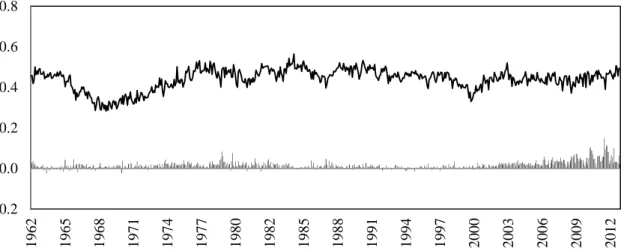
Figure 1. The evolution of tail risk measures for U.S. market
The top black line of the figure reports the evolution of λ(d) for U.S. market. The difference between λ(d) and λ is reported at the bottom of the figure.
The tail risk series starts at a high level, which is possibly related to the Flash Crash of 1962, when the S&P 500 Index declined 22.5% from December 1961 until June 1962. However, during the recent financial crisis of 2007-09, there is no increase in tail risk. This is consistent with Brownlees, Engle and Kelly (2011) who argue that the crisis was followed by inflated volatility that could be predicted by standard volatility forecasting models. Therefore, the effect of soaring volatility is captured by the changes of the constant percentile threshold ut in the tail risk estimation. While the
distribution became wider, the structure of the tail was not different from the previous periods. To explore this pattern in more detail, apart from the entire sample we also consider the period that excludes data after December 2007 in predictive regressions.
The difference between λm(d) and λ is a good evidence to support our idea to change the initial tail risk measure. λ(d) is slightly higher on average due to larger
-0.2 0.0 0.2 0.4 0.6 0.8 1 9 6 2 1 9 6 5 1 9 6 8 1 9 7 1 1 9 7 4 1 9 7 7 1 9 8 0 1 9 8 2 1 9 8 5 1 9 8 8 1 9 9 1 1 9 9 4 1 9 9 7 2 0 0 0 2 0 0 3 2 0 0 6 2 0 0 9 2 0 1 2
8
number of less extreme observations involved in calculation and a lower (in absolute value) average daily threshold. This effect is greater during the recent financial crisis of late 2000s. This happens because our measure is both able to capture how often extreme events are happening during a month instead of concentrating on single shocks and better captures the cross-section effects. Figure 2 exhibits how tail risk is related to future returns.
Figure 2. Tail risk and future returns
The upper panel of the figure presents the left tail risk series (dotted line) and the following twelve-month market excess return (solid line). For better visual effect we standardize both series. The lower panel of the figure presents the historical 10 year rolling window Pearson correlation coefficient with 95% confidence interval.
During almost all the period, tail risk has a positive significant correlation with subsequent market returns. This is consistent with the hypothesis that tail risk is priced by investors. While being risk-averse, a high level of tail risk on the market increases the return required by investors holding a risky portfolio. High persistence of the tail exponent indicates that tail risk shocks are informative about future levels of risk.
-6.0 -4.0 -2.0 0.0 2.0 4.0 1 9 6 2 1 9 6 5 1 9 6 8 1 9 7 1 1 9 7 4 1 9 7 7 1 9 8 0 1 9 8 2 1 9 8 5 1 9 8 8 1 9 9 1 1 9 9 4 1 9 9 7 2 0 0 0 2 0 0 3 2 0 0 6 2 0 0 9 2 0 1 2
Subsequent 12 months market excess returns Left tail risk
1 9 6 2 1 9 6 5 1 9 6 8 1 9 7 1 1 9 7 4 1 9 7 7 1 9 8 0 1 9 8 2 1 9 8 5 1 9 8 8 1 9 9 1 1 9 9 4 1 9 9 7 2 0 0 0 2 0 0 3 2 0 0 6 2 0 0 9 2 0 1 2 -1.0 -0.6 -0.2 0.2 0.6 1.0
9
Therefore, investors dynamically adjust their discount rates in response to the level of tail risk.
In the late 1990s we witness a brief period of negative correlation. This anomaly could be an indicator of the upcoming dot-com bubble because the market did not react adequately to the change of tail risk. However, we find no evidence to support that hypothesis in existing literature and we do not have a sufficient number of similar shocks to prove the hypothesis.
The initial intuition that tail risk can be a solid predictor of future returns comes from the series properties. The variable is highly persistent, i.e., the autoregressive coefficient of order one is 0.88. Regarding the fact, that the monthly tail exponent is measured using non-overlapping data, this high persistentce conveys high predictability of extreme events. Therefore, tail risk can affect the returns both in short- and long-run. Figure 2 provides some visual evidence supporting the idea of significant predictive power of tail risk over future equity premium.
In this paper we intend to evaluate the predictive power of tail risk compared to historical average and other commonly used equity premium predictors. For this purpose we also use variables related to stock market characteristics, interest rates and broad macroeconomic indicators including:
B/M: the book-to-market ratio of the Dow Jones Industrial Average [Pontiff and Schall (1998), Kothari and Shanken (1997)];
The Dividend-Price Ratio (D/P): the difference between the log of 12-month moving sum of dividends paid on the S&P 500 Index and the log of prices;
The Dividend Yield (D/Y): the difference between the log of 12-month moving sum of dividends paid on the S&P 500 Index and the log of lagged prices [Fama and French (1988,1989), Lewellen (2004)];
10
The Dividend Payout Ratio (D/E): the difference between the log of 12-month moving sum of dividends paid on the S&P 500 Index and the log of 12-month moving sum of earnings on the S&P 500 Index [Lamont (1998)];
The Earnings-Price Ratio (E/P): the difference between the log of 12-month moving sum of earnings on the S&P 500 Index and the log of prices [Campbell and Shiller (1988a, 1998)];
Long Term Yield (LTY): Long term U.S. government bond yield [Fama and Schwert (1977), Campbell (1987), Ang and Bekaert (2007)];
The Default Yield Spread (DFS) : the difference between BAA- and AAA- rated corporate bond yields [Campbel (1987)];
The Term Spread (TMS): the difference between long term U.S. government bonds yield and the Treasury bill rate [Fama and French (1989)];
The Realized Stock Variance (SVAR): the sum of squared daily returns on the S&P 500 Index during a month [Guo (2006)];
Net Equity Expansion (NTIS): the ratio of 12-month moving sums of net equity issues by NYSE listed stocks to the total end-of-year market capitalization of NYSE stocks [Baker and Wugler (2000), Boudoukh et al. (2007)];
Inflation (INFL): the Consumer Price Index provided by the Bureau of Labor Statistics [Nelson (1976), Lintner (1975)].6
We consider the same time frame for all predictions to be comparable between each other and to avoid inconsistency. The cross-section width requirement for tail risk estimation implies that predictive regressions only start in July 1962 up to the end of 2012.We present the descriptive statistics for all predictors and correlation coefficients with future excess returns in Table 1.
6
11
Table 1. Descriptive statistics of predictors.
This table reports the descriptive statistics (mean, standard deviation, maximum and minimum) of the predictors for the period of Jul 1962 until Dec 2012. The definition of the predictors can be found Section 3. We also report the Pearson correlation coefficient of the variables with subsequent one- (ρ(rt+1)) and twelve-month (ρ(rt+12)) market
returns. Correlation coefficients marked with * (**) (***) are significant at 10% (5%) (1%) level.
Mean Std. dev. Max Min ρ(rt+1) ρ(rt+12)
λ(d) 0.44 0.05 0.56 0.28 0.11 *** 0.26 *** λ 0.42 0.05 0.56 0.27 0.10 ** 0.21 *** B/M 0.51 0.27 1.21 0.12 0.02 0.08 ** D/P -3.57 0.41 -2.75 -4.52 0.05 0.17 *** D/Y -3.57 0.41 -2.75 -4.53 0.06 0.17 *** DFS (%) 1.04 0.47 3.38 0.32 0.06 0.19 *** TMS (%) 1.78 1.52 4.55 -3.65 0.07 * 0.24 *** D/E -0.75 0.32 1.38 -1.24 0.03 0.14 E/P -2.82 0.45 -1.90 -4.84 0.02 0.06 SVAR (%) 0.22 0.46 7.09 0.01 -0.10 ** 0.10 ** NTIS (%) 1.20 1.94 5.12 -5.76 -0.02 -0.06 INFL (%) 0.33 0.35 1.79 -1.92 -0.08 ** -0.17 *** LTY (%) 6.93 2.54 14.82 2.06 -0.03 0.01
Most of the variables yield significant correlation with future excess returns over subsequent twelve months. The correlation with next month returns is always lower and loses significance for most predictors (except λ(d)). Additionally, λ(d) has the highest (in absolute value) correlation for both time horizons. Although this is an evidence of implicit predictive power, significant Pearson correlation coefficient is not yet a reliable and extensive measure. It does not give any intuition about forecasting errors or relative out-of-sample performance. Therefore, we only can get a possibility of having a predictive power but need to test it with other methodologies.
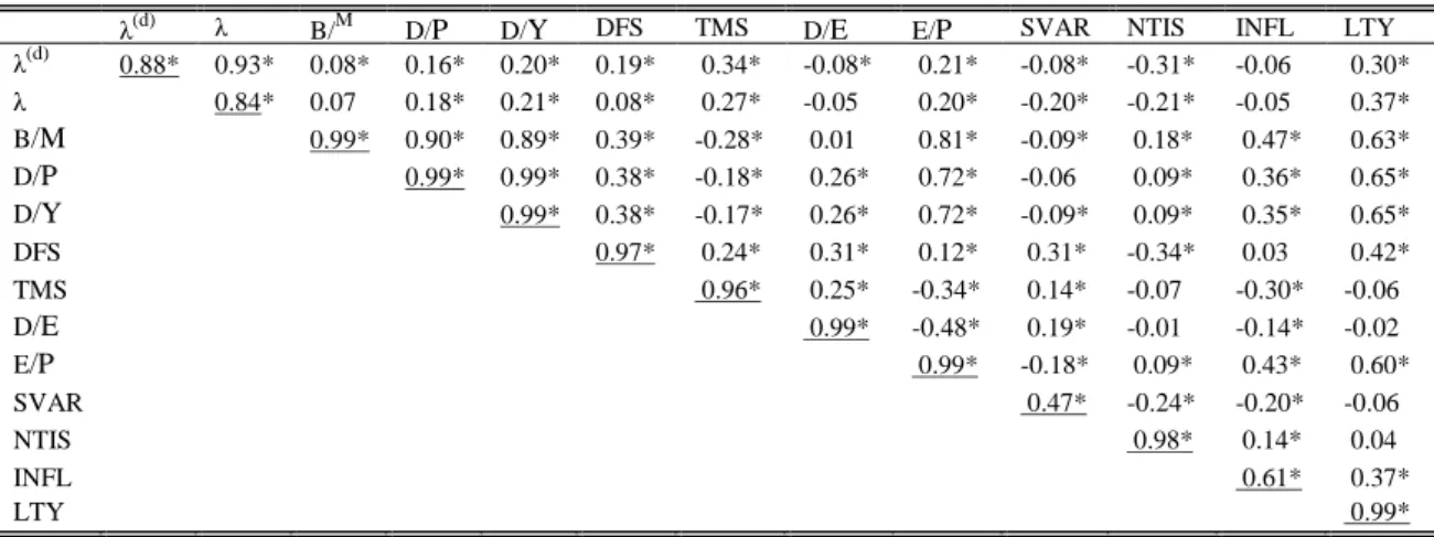
Finally, to evaluate how predictors relate with each other through time we present a correlation matrix of the variables in Table 2. The tail risk has a relatively low correlation with other variables. It is substantial with LTY, NTIS and TMS. All of the variables are very persistent with the lowest serial correlation of 0.47 (SVAR). However, most of them use overlapping data (except λ(d), λ, DFS, TMS, SVAR, INFL and LTY). Therefore, most of the correlations are artificially inflated.
12
Table 2. The correlation matrix of predictors
This table presents the pairwise Pearson correlation coefficients of predictors for the sample dating from Jul 1962 until Dec 2012. The definition of the predictors can be found in the Section 3. The diagonal underlined elements are one-month serial correlation of respective variables.The coefficients significant at 5% level are marked with a star (*).
λ(d) λ
B/M D/P D/Y DFS TMS D/E E/P SVAR NTIS INFL LTY
λ(d) 0.88* 0.93* 0.08* 0.16* 0.20* 0.19* 0.34* -0.08* 0.21* -0.08* -0.31* -0.06 0.30* λ 0.84* 0.07 0.18* 0.21* 0.08* 0.27* -0.05 0.20* -0.20* -0.21* -0.05 0.37* B/M 0.99* 0.90* 0.89* 0.39* -0.28* 0.01 0.81* -0.09* 0.18* 0.47* 0.63* D/P 0.99* 0.99* 0.38* -0.18* 0.26* 0.72* -0.06 0.09* 0.36* 0.65* D/Y 0.99* 0.38* -0.17* 0.26* 0.72* -0.09* 0.09* 0.35* 0.65* DFS 0.97* 0.24* 0.31* 0.12* 0.31* -0.34* 0.03 0.42* TMS 0.96* 0.25* -0.34* 0.14* -0.07 -0.30* -0.06 D/E 0.99* -0.48* 0.19* -0.01 -0.14* -0.02 E/P 0.99* -0.18* 0.09* 0.43* 0.60* SVAR 0.47* -0.24* -0.20* -0.06 NTIS 0.98* 0.14* 0.04 INFL 0.61* 0.37* LTY 0.99*
4
Equity Premium Prediction
4.1 Standard Methodology and Results
Predicting stock returns captures great attention of both academic professionals and financial industry practitioners. Larger degree of accuracy in forecasting would allow investors earning higher returns for investors and increasing the precision of theoretical models. There has been an ongoing debate about equity premium predictability: no evidence on the one side [Goyal and Welch (2008), Bossaerts and Hillion (1999)] and positive evidence on the other [Campbell and Thompson (2008), Lettau and Nieuwerburgh (2008), Ferreira and Santa-Clara (2011), Drechsler and Yaron (2011)].
Various economic variables have been proposed as predictors by the researchers. Apart from the variables used in this paper (see Section 2) academics also use cross-sectional beta premium [Polk et al. (2006)], investment-to-capital ratio [Cochrane (1991)] and consumption-wealth ratio [Lettau and Ludvigson (2005)]. However, there is
13
evidence that all of them fail out-of-sample [Goyal and Welch (2008)]. Because of data unavailability we exclude these variables from our set of equity premium predictors.
We apply the widely used methodology of comparing the sum of squared errors (SSE) of prediction with a SSE of sample average forecast.7 For the initial evaluation of a predictor the in-sample (IS) approach is used. We run a predictive regression, i.e., , where xt is a value of the predictor and ERPt is the equity risk
premium at time t, for the entire sample of available data and compute the R2.
∑
̂
∑ ̅̅̅̅̅̅ (5)
where T is the size of the sample, ̂ is the prediction value from the regression and
̅̅̅̅̅̅is the sample average of the risk premium.
If the R2 is positive, then the predictor forecasts the value of the premium better than historical average. The higher is the R2, the better is the quality of the forecast. While testing predictive power, we firstly evaluate the entire sample and further test the same hypothesis on the smaller sample excluding recent financial crisis of late 2000s. This allows us to make conclusions about predictive power in stable and more turbulent periods. Table 3 presents the in-sample R2s.
Regarding IS forecast, we conclude that tail risk better predicts the equity risk premium for all time horizons compared to other commonly used predictors. It happens in both time frames considered with the exception of high short-term predictive power of inflation when excluding crisis period, however this effect vanishes if we consider the entire sample. This indicates that during turbulent periods historical mean preforms better. Only λ(d)
and TMS are significant in all time horizons and both panels. These results are better regarding tail risk predictive power than our initial expectation. Tail exponents are computed using only recent data instead of rolling sums in case of
7
See Goyal and Welch (2008), Ferreira and Santa-Clara (2011), Campbell and Thompson (2008), Li et al. (2014) and Rapach et al. (2010).
14
valuation ratios, so we expected only good short-term forecasts. Note that the improved tail risk measure (λ(d)) consistently outperforms the initial one (λ), which indicates better capturing of tail distribution properties. This happens mostly during the period of the crisis, because the difference in performance of tail exponents is diminishing in the second panel. For all of the predictors the IS R-squared is always positive and, with several exceptions, increasing with forecast horizon.
Table 3. In-sample results of equity premium prediction
This table presents the In-Sample R2 (in %) of the equity premium predictions for one-month, three-month, one-year and three-year horisons. Panel A provides the results for the entire sample starting form July 1962, while Panel B reports results for the period excluding recent financial crisis. The definition of the predictors can be found Section 3. Coefficients in bold are significant at 5% level based on Clark and West (2007) test of equal forecast ability. We also apply Hodrick’s (1992) standard error correction for overlapping data using 36 lags for three-year forecast horizon and 12 lags for other horizons.
Panel A: 1962:7-2012:12 Panel B: 1962:7-2007:12 1 M 3 M 1 Y 3 Y 1 M 3 M 1 Y 3 Y λ(d) 1.10 1.57 6.93 19.30 1.22 1.95 8.46 22.06 λ 1.05 0.87 4.42 15.73 1.18 1.55 8.08 22.98 B/M 0.04 0.16 0.71 0.01 0.03 0.15 1.04 0.09 D/P 0.26 0.84 3.02 4.40 0.25 0.84 3.48 5.82 D/Y 0.34 0.90 3.02 4.22 0.28 0.84 3.50 5.64 DFS 0.36 1.15 3.77 2.64 0.68 1.34 1.70 0.38 TMS 0.51 1.27 5.82 17.67 0.71 1.68 5.57 14.20 D/E 0.13 0.68 2.03 6.49 0.01 0.04 0.37 3.34 E/P 0.04 0.06 0.31 0.01 0.23 0.72 2.67 2.48 SVAR 0.96 0.05 1.01 0.80 0.14 0.38 0.19 0.00 NTIS 0.04 0.04 0.37 0.01 0.59 1.02 1.44 0.26 INFL 0.63 0.67 2.73 1.11 1.89 2.03 1.41 0.39 LTY 0.06 0.07 0.03 2.15 0.08 0.03 0.69 6.05
However, it is essential to evaluate the out-of-sample predictive power because the conditions closer to real-time forecasting. To predict the value of the risk premium OOS at time t+1, we only use the data available until time t instead of all available sample. Hence, the α and β coefficients of the regression are re-estimated before every prediction.
∑
̂
∑ ̅̅̅̅̅̅ (6) For the OOS forecast we require the initial estimation period m to make the first prediction and afterwards either roll over the estimation period (rolling window) or
15
expand it for the next forecasts (recursive or expanding window), so that we obtain
q=T-m out-of-sample observations. Consistently with Goyal and Welch (2008), we use
expanding window with initial estimation period of twenty years.8 The large estimation period is essential to obtain reliable regression coefficients in the beginning of evaluation period. Also, the number of OOS predictions should be long enough to be representative. To test statistical significance of OOS predictions, we use the Clark and West (2007) test of equal forecast ability. The test helps to identify whether the Mean Squared Percentage Errors (MSPE) of prediction is significantly lower than MSPE of historical average. Practically, this is identical to testing the null hypothesis of R2OOS ≤ 0 against the alternative hypothesis of R2OOS > 0. We apply Hodrick’s (1992) standard error correction for overlapping data using 36 lags for three-year forecast horizon and 12 lags for other horizons.9 Table 4 exhibits the of Out-of Sample R2s.
As expected, the majority of the predictors exhibit a significant reduction in R2 and loss of significance compared to the In-Sample results. The only variable with positive and significant results for all time horizons in both panels is λ(d). Consistently with IS results, INFL yields high predictive power for one-month forecast horizon in Panel B but this is not robust for other time horizons and the entire data sample. We reach the same conclusion with Ang and Bekaert (2009) that term spread is a robust predictor for long-term horizons. The results for tail risk are better if we exclude the crisis from the period, while other variables yield mixed results.
8
To ensure robustness of obtained results in this dissertation, we also evaluate out-of-sample predictions using 120 and 360 months estimation windows with both rolling and expanding windows. All results are quantitavely and qualitatively similar with minor exceptions and are avaliable on request.
9
Richardson and Smith (1991) argue that overlapping return observations bring in the moving average structure into the errors of the forecast, hence jeopardizing the reliability of the tests based on Ordinary Least Squares, and even Newey-West (1987) standard errors. According to Ang and Bekaert (2007), Hodrick’s (1992) standard error correction yields the most conservative test results.
16
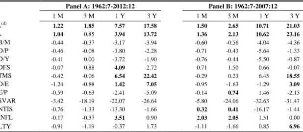
Table 4. Out-of-sample results of equity premium prediction
This table presents the out-of-sample R2 (in %) of the equity premium predictions for month, three-month, one-year and three-one-year horisons. Panel A provides the results for the entire sample starting from July 1962 until December 2012, while Panel B reports results for the period excluding recent financial crisis. The definition of the predictors can be found in Section 3. All predictions are made using expanding window of 240 months. Coefficients in bold are significant at 5% level based on Clark and West (2007) test of equal forecast ability. We also apply Hodrick’s (1992) standard error correction for overlapping data using 36 lags for three-year forecast horizon and 12 lags for other horizons.
Panel A: 1962:7-2012:12 Panel B: 1962:7-2007:12 1 M 3 M 1 Y 3 Y 1 M 3 M 1 Y 3 Y λ(d) 1.22 1.85 7.57 17.58 1.50 2.65 10.71 21.03 λ 1.04 0.85 3.94 13.72 1.36 2.13 10.62 23.16 B/M -0.44 -0.37 -3.17 -3.94 -0.60 -0.56 -4.04 -4.36 D/P -0.46 -0.08 -3.80 -2.28 -0.71 -0.43 -5.64 -1.33 D/Y -0.41 0.00 -3.72 -1.90 -0.76 -0.44 -5.50 -0.87 DFS -0.07 0.88 4.09 2.72 0.71 1.50 0.66 -0.07 TMS -0.42 -0.06 6.54 22.42 -0.29 0.23 6.45 18.55 D/E -1.24 -0.88 1.42 7.05 -0.95 -1.63 -1.29 3.09 E/P -0.59 -0.63 -2.41 -5.09 -0.14 0.74 1.46 -2.15 SVAR -3.42 -18.19 -22.07 -26.64 -5.80 -24.06 -32.63 -31.47 NTIS -0.76 -1.33 -13.30 -1.66 0.32 0.41 -16.17 -1.44 INFL -0.17 -0.37 3.51 0.90 2.03 2.05 1.51 0.00 LTY -0.91 -1.19 -0.37 1.73 -1.11 -1.66 0.85 6.96
Considering the entire sample, we observe that the only robust and significant predictor for one-month horizon is tail risk. Our results also support the view that valuation ratios have lost their predictive power with time.
4.2 Imposing Theoretical Restrictions on Regressions
Despite low predictive power of commonly used predictors in our baseline OOS evaluation, it is premature to conclude that cross-sectional tail risk outperforms other variables. Running predictive regressions with unexpected shocks during initial estimation period might generate unexpected estimates. For instance, such regressions can yield slope coefficients that are inconsistent with theory or negative risk premium forecast. To minimize the effect of such estimation errors, we set simple regression restrictions similar to Campbell and Thompson (2008).
We suggest that investors would rather apply their knowledge of financial theory than simply use statistically measured forecasts. Firstly, we assume that investors would not use perverse coefficients of a regression if they contradict common theory. Every time when the slope sign is different from theoretically expected regression coefficient
17
over the entire sample, we set the slope equal to zero. For example, we expect an increase in D/P to be followed by an increase in prices and, therefore, positive returns. The same intuition should be applied to tail risk, stock variance or interest rate spreads, as investors are risk averse. Secondly, we assume that equity risk premium forecast should be positive as returns of the market are subject to systematic risk which should be compensated with a positive premium. Campbell and Thompson (2008) propose setting ERP to zero when the prediction is negative. As historical equity premium also contains useful information, we suggest using historical average instead of zero. Table 5 exhibits the OOS results after applying regression restrictions.
Table 5. Out-of-Sample results after slope and forecast restrictions
This table presents the out-of-sample R2 (in %) of the equity premium predictions for month, three-month, one-year and three-one-year horisons. Panel A provides the results for the entire sample starting from July 1962 until December 2012, while Panel B reports results for the period excluding recent financial crisis. The definition of the predictors can be found in Section 3. All predictions are made using expanding window of 240 months. Coefficients in bold are significant at 5% level based on Clark and West (2007) test of equal forecast ability. We also apply Hodrick’s (1992) standard error correction for overlapping data using 36 lags for three-year forecast horizon and 12 lags for other horizons.
Panel A: 1962:7-2012:12 Panel B: 1962:7-2007:12 1 M 3 M 1 Y 3 Y 1 M 3 M 1 Y 3 Y λ(d) 1.06 1.54 6.63 15.56 1.34 2.44 9.22 18.34 λ 0.91 0.85 5.14 14.66 1.01 2.16 9.33 20.55 B/M -0.47 -0.66 -4.74 -4.28 -0.63 -0.97 -6.23 -4.79 D/P 0.30 0.22 -1.34 -6.27 0.31 0.00 -2.18 -5.91 D/Y 0.35 0.93 -0.66 -5.80 0.27 0.87 -1.20 -5.34 DFS 0.14 1.33 4.09 2.54 0.99 2.13 0.66 -0.28 TMS -0.27 -0.15 6.54 22.42 -0.08 0.11 6.45 18.55 D/E -0.40 -0.46 0.47 3.91 -0.69 -1.62 -2.63 -0.51 E/P 0.13 0.36 0.80 -4.32 -0.31 -0.71 -0.87 -1.26 SVAR -3.64 -17.80 -22.07 -26.69 -5.02 -24.06 -32.63 -31.58 NTIS -0.46 -0.89 -11.43 -1.50 0.67 0.94 -13.61 -1.59 INFL -0.50 -0.59 3.51 0.77 1.51 2.21 1.51 -0.16 LTY -0.24 -0.33 -8.79 -8.23 -0.20 -0.36 -10.57 -4.10
After imposing slope and forecast restriction on predictive regressions we obtain mixed results. The forecast accuracy of valuation ratios (D/P, D/Y, D/E and E/P) and long term yield increased for short term forecast horizons. For the majority of predictors, the OOS R2 shrinks for one- and three-year forecasts. These results imply that statistical methodology is more powerful than theoretical restrictions in these cases. Several variables are almost unaffected by restrictions or exhibit small insignificant
18
change in predictive power (λ, B/M, TMS, DFS, NTIS, and SVAR). The only variable that is significantly negatively affected by restrictions is INFL.
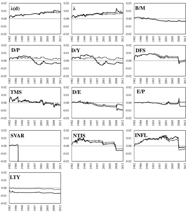
Figure 3. Out-of-Sample performance of one-month horizon predictions
This figure presents the difference between the cumulative forecast SSE of the historical mean and the respective predictors. Solid line stands for initial OOS results while dotted line represents results with slope and prediction restrictions.Positive slope of the line means that predictor outperforms the historical average. All forecasts use an expanding window of 240 months. The definition of the predictors can be found Section 3.
Tail risk still remains the most robust equity risk premium predictor and is still significant for all forecast horizons. None of the predictors is able to yield a comparable
-0.02 -0.01 0.00 0.01 0.02 198 2 198 6 199 0 199 3 199 7 200 1 200 5 200 8 201 2 λ(d) -0.02 -0.01 0.00 0.01 0.02 198 2 198 6 199 0 199 3 199 7 200 1 200 5 200 8 201 2 λ -0.02 -0.01 0.00 0.01 0.02 198 2 198 6 199 0 199 3 199 7 200 1 200 5 200 8 201 2 B/M -0.02 -0.01 0.00 0.01 0.02 198 2 198 6 199 0 199 3 199 7 200 1 200 5 200 8 201 2 D/P -0.02 -0.01 0.00 0.01 0.02 198 2 198 6 199 0 199 3 199 7 200 1 200 5 200 8 201 2 D/Y -0.02 -0.01 0.00 0.01 0.02 198 2 198 6 199 0 199 3 199 7 200 1 200 5 200 8 201 2 DFS -0.02 -0.01 0.00 0.01 0.02 198 2 198 6 199 0 199 3 199 7 200 1 200 5 200 8 201 2 TMS -0.02 -0.01 0.00 0.01 0.02 198 2 198 6 199 0 199 3 199 7 200 1 200 5 200 8 201 2 D/E -0.02 -0.01 0.00 0.01 0.02 198 2 198 6 199 0 199 3 199 7 200 1 200 5 200 8 201 2 E/P -0.02 -0.01 0.00 0.01 0.02 198 2 198 6 199 0 199 3 199 7 200 1 200 5 200 8 201 2 SVAR -0.02 -0.01 0.00 0.01 0.02 198 2 198 6 199 0 199 3 199 7 200 1 200 5 200 8 201 2 NTIS -0.02 -0.01 0.00 0.01 0.02 198 2 198 6 199 0 199 3 199 7 200 1 200 5 200 8 201 2 INFL -0.02 -0.01 0.00 0.01 0.02 198 2 198 6 199 0 199 3 199 7 200 1 200 5 200 8 201 2 LTY
19
value of R2 for one- and three-month forecast horizons. Only TMS yields a better predictive ability for long time horizon.
Figure 3 presents the evolution of forecasting performance of predictors for a one-month horizon.10 We can conclude that only cross-sectional tail risk consistently better predicts the equity premium compared to historical average as the difference in SSE is increasing with time. After restricting the slope and forecast, D/Y and D/P also have lower cumulative SSE than historical mean for all the period. NTIS, INFL and DFS were performing well until recent financial crisis but then suffered a large shock in the second half of 2008. This indicates that during the preiods of unexpected extreme downturns those predictors are not able to outperform the historical mean.
4.3 Combination of individual predictors
We further make and attempt to improve the predictive power by combining the forecasts of different variables and determine if any combination approach outperforms the cross-sectional tail risk. Because of high correlation between predictors it is not recommended to use variables simultaneously in a predictive regression due to multicollinearity. Therefore, we study alternative methods of combination.
One of the first extensive studies on forecast combinations is conducted by Bates and Granger (1969). They show that combinations of forecasts are able to outperform individual predictions. Applying this to financial theory, Mamaysky et al. (2007, 2008) conclude that the predictability of mutual funds’ alphas and betas significantly increases by combining forecast of a predictive regression with Kalman filter model. Furthermore, the positive effects of forecast combinations are also affirmed by Rapach
et al. (2010) using a broad set of predictors.
20
The intuition under combining different predictions together is straight forward. Every predictor carries some set of useful information that allows forecasting future excess returns. Combination of forecasts aims to capture all beneficial information in a single aggregated forecast which potentially has higher predictive power. Moreover, similarly to asset allocation, adding new predictors to ‘forecasting portfolio’ should reduce the variance of equity premium forecasts. Table 6 presents correlation matrix of individual predictions.
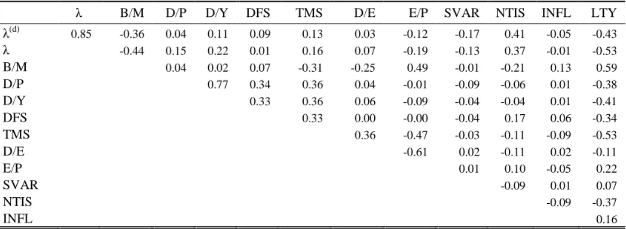
Table 6. Correlation matrix of OOS equity premium forecasts
This table presents pairwise Pearson correlation coefficients of one-month horizon equity premium forecasts for the period starting from July 1962 until December 2012. All OOS forecasts use 240 months expanding window. The definition of the predictors can be found in Section 3.
λ B/M D/P D/Y DFS TMS D/E E/P SVAR NTIS INFL LTY λ(d) 0.85 -0.36 0.04 0.11 0.09 0.13 0.03 -0.12 -0.17 0.41 -0.05 -0.43 λ -0.44 0.15 0.22 0.01 0.16 0.07 -0.19 -0.13 0.37 -0.01 -0.53 B/M 0.04 0.02 0.07 -0.31 -0.25 0.49 -0.01 -0.21 0.13 0.59 D/P 0.77 0.34 0.36 0.04 -0.01 -0.09 -0.06 0.01 -0.38 D/Y 0.33 0.36 0.06 -0.09 -0.04 -0.04 0.01 -0.41 DFS 0.33 0.00 -0.00 -0.04 0.17 0.06 -0.34 TMS 0.36 -0.47 -0.03 -0.11 -0.09 -0.53 D/E -0.61 0.02 -0.11 0.02 -0.11 E/P 0.01 0.10 -0.05 0.22 SVAR -0.09 0.01 0.07 NTIS -0.09 -0.37 INFL 0.16
We observe many low and negative correlation coefficients, which carries large potential benefits. Portfolio theory suggests that low and negative correlations between combination components should greatly reduce the volatility of predictions. However, the variance reduction of the combined forecast can be overruled by increasing estimation errors.
The debate about the most efficient way of combining predictions remains unsolved. Elliott et al. (2013) suggest a complete subset regressions approach which aims to find a tradeoff between the model complexity and estimation errors by applying a methodology similar to efficient frontier construction. Stock and Watson (2004) compute the weights of predictions within a combination based on historical forecasting performance of individual models over OOS estimation period. Hsiao and Wan (2014)
21
consider several geometric approaches of combining forecasts in large samples. Raftery
et al. (1997) develop an Occam’s Window methodology to exclude least useful
prediction models from the subset and further averaging the predictions. Elliott and Timmermann (2005) set the combination weights driven by Markov regime switching process.
However, there is also a set of literature suggesting that simple combining methods commonly perform better than more complex approaches [Timmermann (2006), Rapach et al. (2010) and Elliott and Drive (2011)]. We support this view as errors introduced by estimation of the combination weights might overpower any gains from setting the weights closer to their optimal values.
The general combination of forecasts takes the following form:
∑ (7)
where N is a number of individual predictions to combine; ωi,t is ex ante combining
weight of ith individual prediction defined at time t.
We suggest four simple combination methods. Combination (1) is a simple average of all individual forecasts [ωi,(1) = 1/N for i = 1,...,N in (7)]. Combination (2) is
a trimmed mean that assigns zero weights to the largest and the smallest predictions
[ωi,(2) = 1/(N-2) for i = 2,...,N-1 in (7)]. Combination (3) is a trimmed mean that assigns
zero weights to the three largest and smallest predictions [ωi,(3) = 1/(N-6) for i =
4,...,N-3 in (7)]. And, finally, Combination (4) is a median of all predictions. We firstly test if the combination of all predictors excluding tail risk can out-of-sample outperform the latter. Afterwards, we include tail risk into the set of predictors to check if it has significant complementary predictive power. Table 7 presents the OOS results of mentioned forecast combinations.
22
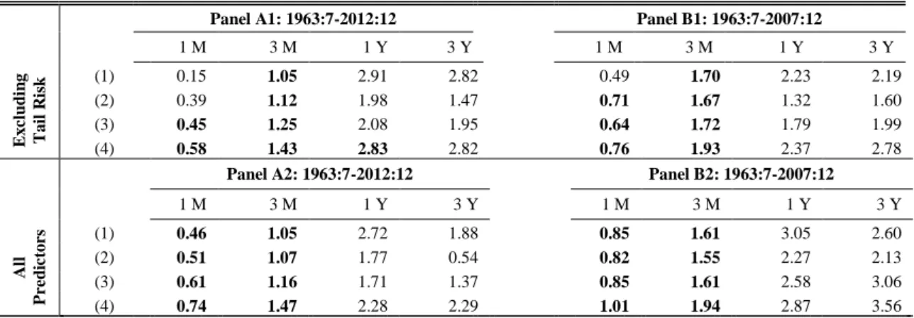
Table 7. Out-of-sample results of combining predictors
This table presents the out-of-sample R2 (in %) of the equity premium predictions for month, three-month, one-year and three-one-year horisons. Panels A1 and A2 provide the results for the entire sample starting from July 1962 until December 2012, while Panels B1 and B2 report results for the period excluding recent financial crisis. Panels A1 and B1 report results of combining all 13 predictors (see Section 2), while Panels A2 and B2 report results of combining predictors excluding tail risk measures. Combination (1) is a simple average of predictions. Combination (2) is an average of all predictions excluding the highest and the lowest values. Combination (3) excludes the three largest and the three smallest predictions from the combination and averages the rest. Combination (4) is the median of all predictions. All predictions are made using expanding window of 240 months. Coefficients in bold are significant at 5% level based on Clark and West (2007) test of equal forecast ability. We also apply Hodrick’s (1992) standard error correction for overlapping data using 36 lags for three-year forecast horizon and 12 lags for other horizons.
Panel A1: 1963:7-2012:12 Panel B1: 1963:7-2007:12
1 M 3 M 1 Y 3 Y 1 M 3 M 1 Y 3 Y E x cl u d in g T a il R isk (1) 0.15 1.05 2.91 2.82 0.49 1.70 2.23 2.19 (2) 0.39 1.12 1.98 1.47 0.71 1.67 1.32 1.60 (3) 0.45 1.25 2.08 1.95 0.64 1.72 1.79 1.99 (4) 0.58 1.43 2.83 2.82 0.76 1.93 2.37 2.78
Panel A2: 1963:7-2012:12 Panel B2: 1963:7-2007:12
1 M 3 M 1 Y 3 Y 1 M 3 M 1 Y 3 Y A ll Pr ed ic to rs (1) 0.46 1.05 2.72 1.88 0.85 1.61 3.05 2.60 (2) 0.51 1.07 1.77 0.54 0.82 1.55 2.27 2.13 (3) 0.61 1.16 1.71 1.37 0.85 1.61 2.58 3.06 (4) 0.74 1.47 2.28 2.29 1.01 1.94 2.87 3.56
From Panels A1 and B1 we conclude that naïve combinations of all predictors excluding cross-sectional tail risk outperform individual components but are unable to beat λ(d) in neither of time periods considered. Moreover, Panels A2 and B2 suggest that even combining tail risk with other predictors yields lower R2 than individual forecasts with λ(d). Note that the fewer predictions are averaged in a combination, the better are the results, namely Combination (1) < (2) < (3) < (4) consistently in all panels (with two minor exceptions). The results indicate that while combining tail risk with other predictors, the estimation noise distorts the predictive power more than the benefits of reduction in the volatility of the estimates.
However, the correlation matrix of predictions and the individual OOS results suggest that it might be more beneficial not to include predictors with poor performance into the combination. But this creates an in-sample bias of choosing ex post good predictors for a combination. A monthly weighting methodology based on previous out-of-sample performance would be infeasible due to overlapping data for three-month, one-year and three-year forecasts. We do not perform this analysis only for one-month
23
horizon forecasts to be consistent throughout the paper. Instead, we suggest testing if some model can provide useful information beyond that already contained in tail risk. Consider an optimal forecast combination between two models i and j:
̂ (8)
where 0 ≤ θ ≤ 1. If θ = 0 then model i encompasses model j that does not contain any additional useful information. Harvey, Leybourne and Newbold (1998) developed a statistic that tests if the forecast given by a model i encompasses the forecast given by an alternative model j or, in other words, if θ = 0. Table 8 presents the p-values of pairwise tests.
Table 8. Pairwise forecast encopassing test results
This table presents p-values for the Harvey, Leybourne and Newbold (1998) MHLN statictic of one-month horizon forecasts. The statistic corresponds to a test of the null hypothesis that the forecast given by the predictor in a column heading encompasses the forecast given by the predictor in a row heading. The forecast period starts from July 1962 and ends in December 2012. All forecasts use 240 months expanding window. Combination (1) is an average of all forecasts and combination (4) is a median of all forecasts. The definition of the remaining variables can be found in Section 3.
λ(d) λ B/M D/P D/Y DFS TMS D/E E/P SVAR NTIS INFL LTY (1) (4)
λ(d) 0.21 0.00 0.03 0.04 0.04 0.02 0.00 0.02 0.11 0.01 0.02 0.01 0.04 0.10 λ 0.55 0.01 0.05 0.06 0.05 0.02 0.01 0.03 0.11 0.01 0.03 0.01 0.09 0.16 B/M 0.72 0.60 0.81 0.81 0.50 0.10 0.22 0.90 0.18 0.05 0.09 0.49 0.85 0.96 D/P 0.47 0.40 0.03 0.47 0.22 0.05 0.05 0.20 0.14 0.02 0.04 0.07 0.43 0.68 D/Y 0.46 0.39 0.03 0.33 0.21 0.04 0.05 0.18 0.13 0.02 0.04 0.07 0.39 0.64 DFS 0.58 0.45 0.10 0.35 0.38 0.06 0.08 0.28 0.14 0.03 0.03 0.13 0.50 0.66 TMS 0.57 0.49 0.06 0.19 0.21 0.19 0.11 0.13 0.12 0.04 0.08 0.11 0.35 0.41 D/E 0.84 0.75 0.18 0.55 0.58 0.41 0.16 0.41 0.17 0.05 0.11 0.30 0.84 0.91 E/P 0.58 0.46 0.03 0.44 0.46 0.29 0.05 0.06 0.15 0.03 0.06 0.12 0.57 0.80 SVAR 0.86 0.83 0.68 0.77 0.78 0.75 0.60 0.70 0.78 0.48 0.56 0.77 0.85 0.87 NTIS 0.62 0.53 0.05 0.13 0.15 0.16 0.06 0.06 0.14 0.12 0.05 0.09 0.30 0.33 INFL 0.52 0.46 0.09 0.20 0.22 0.19 0.13 0.12 0.18 0.14 0.06 0.18 0.39 0.44 LTY 0.81 0.66 0.16 0.53 0.55 0.38 0.10 0.17 0.60 0.18 0.05 0.10 0.88 0.96 (1) 0.73 0.56 0.01 0.21 0.25 0.16 0.05 0.02 0.14 0.14 0.02 0.04 0.02 0.92 (4) 0.46 0.32 0.00 0.10 0.13 0.09 0.03 0.01 0.06 0.13 0.01 0.03 0.01 0.04
The first two columns of the table indicate that none of other individual models can provide useful information for the forecasts with tail risk. Therefore, we should not expect any noticeable improvement even using more complex forecast combination methodologies to reduce the weights of poor-performing models. In other columns of the table we observe a number of rejected tests, which supports the results of Table 7 and provides evidence that combinations can be beneficial for other predictors. Note
24
that Combination (4), which is a median of all predictions, encompasses the mean model and not vice-versa. It suggests that some of the predictors included in Combination (1) not only fail to contribute but actually harm combination by adding estimation noise and distorting the forecasts.
5
Predictive Power and Real Economy
So far our results provide evidence that the cross-sectional tail risk is the most powerful individual predictor that outperforms all other predictors commonly used in academic literature. Moreover, different forecast combinations are also not able to outperform predictions made by tail risk. In this section we aim to link the predictive power with the state of real economy. Our intent is to test whether high performance of tail risk measure is caused by some particular state of business cycle or economy growth.
Firstly, we use the data provided by National Bureau of Economic Research (NBER) which defines the periods of expansions and contractions.11 According to NBER, during the OOS forecast period the troughs (peaks) of business cycles occur in November 1982 (July 1990), March 1991 (March 2001), November 2001 (December 2007) and June 2009. As a result, the period consists of 38 months of recession and 327 months of expansion. Table 9 presents the OOS prediction results in various business cycles phases.
Most of the predictors (except NTIS, INFL and LTY) yield higher predictive power during the periods of contraction considering short horizon forecasts. Regarding longer horizon forecast the exceptions to this tendency are INFL, TMS and λ(d). The higher performance of predictors during recessions is consistent with findings of
11
25
Cochrane (2005) and Fama and French (1989) who claim that increasing risk aversion during such periods inflates the risk premium demanded by investors, consequently triggering high predictability of equity premium.
Table 9. The OOS results during different business cycle stages
This table presents the out-of-sample R2 (in %) of the equity premium predictions for month, three-month, one-year and three-one-year horisons. The forecast period starts from July 1962 and ends in December 2012. All forecasts use 240 months expanding window. Panel A provides the results for the periods of contractions defined by NBER, while Panel B reports results for the periods of expansions. The definition of predictors can be found in Section 3. The cominations of forecasts are named as followed: (1) is an average of all forecasts; (2) is a trimmed mean (excluding the largest and the smallest forecast values); (3) is a trimmed mean (excluding the three largest and the three smallest forecast values); (4) is a median of all forecasts. Coefficients in bold are significant at 5% level based on Clark and West (2007) test of equal forecast ability. We also apply Hodrick’s (1992) standard error correction for overlapping data using 36 lags for three-year forecast horizon and 12 lags for other horizons.
Panel A: Contractions Panel B: Expansions
1 M 3 M 1 Y 3 Y 1 M 3 M 1 Y 3 Y λ(d) 3.07 2.97 5.82 7.11 0.47 0.91 7.00 16.66 λ 3.22 1.91 3.61 -4.04 0.23 0.38 5.84 17.10 B/M 0.62 1.52 6.18 0.11 -0.79 -1.63 -9.76 -4.86 D/P 2.81 5.69 13.82 12.54 -0.44 -2.21 -8.33 -8.72 D/Y 3.53 6.41 14.13 10.84 -0.58 -1.50 -7.47 -7.97 DFS 0.36 4.03 16.99 26.68 0.08 0.12 -1.86 -0.61 TMS 1.86 3.08 4.03 22.13 -0.89 -1.59 7.70 22.46 D/E 1.53 5.05 15.83 47.17 -0.97 -2.92 -6.61 -1.74 E/P 2.25 3.74 8.65 -23.14 -0.49 -1.14 -2.82 -1.86 SVAR 0.21 0.55 6.12 10.57 -4.78 -25.97 -35.05 -31.55 NTIS -1.21 0.69 8.29 9.84 -0.24 -1.59 -20.52 -2.98 INFL -7.89 -8.40 1.92 0.64 1.68 2.89 4.24 0.78 LTY -0.65 -0.87 5.21 0.00 -0.12 -0.08 -15.24 -9.30 (1) 0.82 2.64 8.98 6.37 0.36 0.35 -0.16 1.29 (2) 1.12 2.86 7.69 0.11 0.33 0.28 -0.95 0.60 (3) 1.44 2.91 6.42 0.07 0.37 0.38 -0.46 1.54 (4) 1.69 2.84 8.08 4.71 0.46 0.86 -0.40 1.98
Although forecasts by tail risk are outperformed by D/Y during the periods of contraction and by INFL during the periods of expansion, our measure is the only one yielding positive and significant R2 considering both states of economy and all forecast horizons. This is another evidence of robustness of equity premium predictions generated by lower tail risk.
Secondly, we consider real GDP growth as an indicator of the economy state.12 We split the entire sample by the periods of low, normal and high GDP growth. To ensure sufficient number of observations for every sample, we follow the approach
12
The data is provided by U.S. Department of Commerce: Bureau of Ecvonomic Analysis and is available at: http://www.bea.gov/national/index.htm#gdp. As the U.S. GDP data is only available on a quarterly basis, we assume constant growth during all three months of a quarter.
26
described in Rapach et al. (2010) and Liew and Vassalou (2000) by sorting the sample by real GDP growth and using the bottom, middle and top terciles as the respective thresholds. Intuitively, during the periods of normal growth, the historical average is anticipated to perform relatively well as there are less systematic shocks. Therefore, we presume better predictive power for the rest of predictors during periods of high and low economy growth. The results are presented in Table 10.
The valuation and payout ratios perform considerably better during periods of low economy growth. Most of other variables, opposing to our initial intuition, yield better results during the periods of normal growth. The distinctive performance of tail risk measure is mainly attributed to mentioned stages. As an exception from the set of predictors, the only variable that yields positive OOS R2 for all forecast horizons in high growth periods is INFL.
Table 10. OOS results during different GDP growth periods
This table presents the out-of-sample R2 (in %) of the equity premium predictions for month, three-month, one-year and three-one-year horisons. The forecast period starts from July 1962 and ends in December 2012. All forecasts use 240 months expanding window. Panel A (B, C) provides the results for the periods with low (normal, high) GDP growth. The definition of predictors can be found in Section 3. The cominations of forecasts are named as followed: (1) is an average of all forecasts and combination; (2) is a trimmed mean (excluding the largest and the smallest forecast values); (3) is a trimmed mean (excluding the three largest and the three smallest forecast values); (4) is a median of all forecasts. Coefficients in bold are significant at 5% level based on Clark and West (2007) test of equal forecast ability. We also apply Hodrick’s (1992) standard error correction for overlapping data using 36 lags for three-year forecast horizon and 12 lags for other horizons.
Panel A: Low growth Panel B: Normal Growth Panel C: High Growth
1 M 3 M 1 Y 3 Y 1 M 3 M 1 Y 3 Y 1 M 3 M 1 Y 3 Y λ(d) 1.55 1.78 6.18 14.63 3.67 5.48 11.27 13.73 -0.99 -1.29 2.47 18.14 λ 1.41 1.20 4.28 12.34 3.99 4.99 11.68 13.86 -1.42 -2.31 -0.06 17.79 B/M 0.00 0.51 1.04 -2.21 -2.53 -3.72 -8.51 1.84 -0.09 -0.80 -17.42 -11.85 D/P 1.19 3.05 6.86 -5.35 -0.69 -1.05 -6.24 -10.78 -0.50 -3.92 -19.92 -3.26 D/Y 1.49 3.67 7.43 -5.11 -0.83 -0.05 -2.34 -9.70 -0.71 -3.24 -22.71 -3.10 DFS 0.34 3.18 9.56 7.72 1.05 -0.77 0.11 0.48 -0.63 -0.62 -7.47 -1.08 TMS 1.27 3.11 7.33 25.61 3.46 0.26 9.18 22.05 -4.46 -6.10 1.06 19.40 D/E 0.37 2.38 7.12 21.47 -1.37 -2.02 -6.04 -9.70 -1.04 -4.48 -11.58 -2.51 E/P 0.89 1.27 4.11 -13.42 -0.71 -0.38 -0.16 0.98 -0.56 -0.76 -7.90 0.57 SVAR 0.13 -0.15 3.44 3.33 0.34 -1.99 -3.48 -0.94 -11.27 -58.45 -119.96 -80.88 NTIS -1.43 -2.29 -6.50 0.71 2.79 -0.47 -21.79 0.13 -0.72 1.31 -13.78 -5.25 INFL -3.65 -4.97 1.97 1.41 3.46 4.74 2.96 -0.33 2.11 3.77 8.73 1.06 LTY -0.52 -0.62 0.12 -2.82 -0.53 -1.33 -17.65 -14.36 0.31 0.80 -24.78 -8.50 (1) 0.47 1.93 5.23 3.78 1.62 2.12 3.29 1.64 -0.15 -1.15 -5.40 0.10 (2) 0.63 2.18 4.68 1.03 1.28 1.56 1.90 1.41 -0.07 -1.15 -7.03 -0.73 (3) 0.84 2.32 4.09 0.89 1.27 1.56 2.73 3.34 -0.07 -1.12 -6.56 0.14 (4) 1.04 2.68 4.82 3.15 1.72 2.17 2.29 3.86 -0.20 -1.08 -5.31 0.02
27
6
Economic Interpretation of R
2Throughout the paper we show that lower tail risk is a significant and robust predictor of equity risk premium. In different model specifications the OOS R2 of one-month horizon prediction ranges between 0.57% and 1.22%. The same measure reaches up to 17.58% for the three-year horizon predictions. Following Campbell and Thompson (2008) we further set a link between predictive power and asset allocation in a simple mean-variance framework.
Consider the equity risk premium process as following:
̅̅̅̅̅̅ (9)
where ̅̅̅̅̅̅ is unconditional average market excess return, xt is a predictor variable with
a mean of 0 and the variance of σ2x and εt+1 is an error term with a mean of 0 and the
variance of σ2ε.
If an investor with a single-period investment horizon and a mean variance utility function does not observe xt and invests in a risky market portfolio and a riskless
asset, the optimal weight in a risky portfolio would be:13
( ) ( ̅̅̅̅̅̅ ) (10)
where γ is a coefficient of relative risk aversion. The investor earns excess return of
( ) ( ̅̅̅̅̅̅ ) (11)
where SR is unconditional Sharpe ratio of a market portfolio. Now consider the case when the investor actually observes xt. This will decrease the denominator in Equation
(11) as σ2xt portion of variance is now observable. The optimal weight and excess return
become:
13
Because there is no closed form formula for optimal weights for alternative utility functions that account for higher moments, we only focus on the mean-variance case for simplification reasons. We expect similar qualitative results using more complex utility functions.
28
( ) ( ̅̅̅̅̅̅
) (12)
( ) ( ̅̅̅̅̅̅ ) ( ) ( ) (13)
where R2 = σ2x / (σ2x + σ2ε) is the R2 statistic of the ERP predictive regression using xt.
By observing xt. the investor gains the difference between r* and r:
( ) ( ) (14)
The proportional increase of expected return is:
( ) ( ) (15)
Note that the correct way of evaluating the OOS R2 statistic is to compare it with the squared Sharpe ratio of the asset (which is being predicted) with the frequency matching the forecast. In our sample, the monthly Sharpe ratio of CRSP Value-Weighted Index is 0.11, corresponding to the values of 0.18, 0.37 and 0.63 for three-month, one-year and three-year frequencies respectively. We use a simplified assumption of zero serial correlation of market return to adjust the frequency of the Sharpe ratio. Figure 4 presents relative improvement of the mean-variance asset allocation by using positive OOS R2.
This analysis shows that even low R2 can yield substantial improvements in expected returns. The R2 of 1.06% for next-month predictions by λ(d) more than doubles expected returns. The cross-sectional tail risk generates highest gains for one-month horizon forecasts. This results are in line with our expectations because the measure is estimated only using the data of current month and is highly persistent. The gains from using tail risk predictor for longer forecast horizons are smaller but still substantial and range between 50% and 65%.