UNIVERSIDADE DE ÉVORA
DEPARTAMENTO DE ECONOMIA
DOCUMENTO DE TRABALHO Nº
2005/05
March
Goodness of Fit Tests for Moment Condition Models*
Joaquim J. S. Ramalho
Universidade de Évora, Departamento de Economia
Richard J. Smith
Cemmap, I.F.S. and U.C.L. and, Department of Economics - University of Warwick
*Aspects of this research were presented at the 2002 Econometric Society European Meetings, Venice. Smith gratefully acknowledges financial support for his research from a 2002 Leverhulme Major Research Fellowship.
UNIVERSIDADE DE ÉVORA DEPARTAMENTO DE ECONOMIA
Largo dos Colegiais, 2 – 7000-803 Évora – Portugal Tel.: +351 266 740 894 Fax: +351 266 742 494
Abstract:
This paper proposes novel methods for the construction of tests for models specified by unconditional moment restrictions. It exploits the classical-like nature of generalized empirical likelihood (GEL) to define Pearson-type statistics for over-identifying moment conditions and parametric constraints based on constrasts of GEL implied probabilities which are natural by-products of GEL estimation. As is increasingly recognized, GEL can possess both theoretical and empirical advantages over the more standard generalized method of moments (GMM). Monte Carlo evidence comparing GMM, GEL and Pearsontype statistics for over-identifying moment conditions indicates that the size properties of a particular Pearson-type statistic is competitive in most and an improvement over other statistics in many circumstances.
Palavras-chave/Keywords: GMM, Generalized Empirical Likelihood, Overidentifying Moments,
Parametric Restrictions, Pearson-Type Tests
1
Introduction
This paper proposes novel methods for the construction of tests for models specified by unconditional moment restrictions. The generalized method of moments (GMM), Hansen (1982), is the conventional method of fit for such models. In view of increasing Monte Carlo evidence indicating that GMM estimators may be badly biased in finite samples and that the empirical and nominal size of associated tests may differ substantially, see, for example, the Special Issue of the Journal of Business & Economic Statistics (July 1996), a number of alternative estimators which are asymptotically first-order equivalent to efficient GMM have been suggested. These estimators include empirical likelihood (EL) [Qin and Lawless (1994), Imbens (1997), Owen (2001)], exponential tilting (ET) [Kitamura and Stutzer (1997) and Imbens, Spady and Johnson (1998)] and the continuous updating estimator (CUE) [Hansen, Heaton and Yaron (1996)].
These estimators share a common structure, being members of a class of generalized empirical likelihood (GEL) estimators [Newey and Smith (2004) and Smith (1997, 2001)]. GEL estimation seems to possess many attractive theoretical features relative to GMM. Large sample analysis, Newey and Smith (2004), indicates that GEL estimators may be less prone to bias than those based on GMM. GEL also appears to have diverse advantages over GMM in finite samples. Imbens (1997) and Newey, Ramalho and Smith (2002) report promising Monte Carlo results concerning the small sample bias of GEL estimators, while Imbens, Spady and Johnson (1998) find that particular GEL tests of overidentifying moment conditions, although also oversized in finite samples, possess actual sizes closer to nominal size than Hansen’s (1982) test.
GEL bears certain similarities to likelihood-based methods, allowing the construc-tion of classical-type tests of hypotheses in the moment condiconstruc-tion framework. These include overidentifying moment conditions, for which only Hansen’s (1982) test is typi-cally available in the GMM setting. This paper exploits the classical-like feature of GEL and proposes new specification tests for moment condition models similar in spirit to the standard Pearson tests for goodness of fit. In particular, a set of implied or
em-pirical probabilities which incorporate the moment condition information are associated with each GEL estimator, which by reweighting the data impose exactly all moment conditions on the sample, rather than particular linear combinations as in the GMM case. See Newey and Smith (2004). Implied probabilities based on GMM may also be be constructed in a likewise fashion by utilising the GEL criterion function evaluated at an efficient GMM estimator as discussed in Brown and Newey (1992, 2003). The resultant GEL distribution function estimator formed from the implied probabilities is an efficient estimator of the distribution of the data, in particular, it dominates the em-pirical distribution function (EDF) implicitly used by GMM. Contrasts between GEL implied and EDF probabilities allow the construction of classical Pearson-type tests of over-identifying moment conditions. A similar approach can be used to construct tests for parametric restrictions based on contrasts of restricted and unrestricted GEL implied probabilities.
In a set of Monte Carlo experiments based on those considered in Imbens, Spady and Johnson (1998), we compare the finite sample size behaviour of Pearson-type statistics for over-identifying moment conditions with other existing GMM and GEL tests, such as Hansen’s (1982) test and those proposed in Smith (1997).
This paper is organized as follows. Section 2 briefly reviews GMM and GEL estima-tion. Pearson-type tests for over-identifying moment conditions are presented in section 3 while parametric restrictions are considered in section 4. The Monte Carlo experiments are discussed in section 5. Section 6 concludes. Proofs of the results contained in the paper are provided in the Appendix.
2
The Model and Estimators
This section briefly reconsiders the model and estimators. The set-up considered and notation used here is similar to that in Newey and Smith (2004), which is henceforth abbreviated as NS.
the k-vector z. Also, let g(z, β) be an m-vector of known functions of the data observation z and the p-vector of parameters β, where m ≥ p. The model has a true parameter β0
satisfying the unconditional moment condition
E[g(z, β0)] = 0, (2.1)
where E[.] denotes expectation taken with respect to the distribution of z.
Various methods of estimation have been proposed for models specified by moment conditions of the type (2.1). The standard method is two-step GMM estimation, see Hansen (1982). Let gi(β)≡ g(zi, β), ˆg(β)≡
Pn
i=1gi(β)/n and ˆΩ(β)≡
Pn
i=1gi(β)gi(β)0/n
or the centred estimatorPni=1[gi(β)− ˆg(β)][gi(β)− ˆg(β)]0/n. Also, let ˜β be some
prelim-inary estimator given by ˜β = arg minβ∈Bˆg(β)0Wˆ−1g(β) whereˆ B denotes the parameter
space and ˆW is a random matrix with properties to be specified below. The two-step efficient GMM estimator is defined by
ˆ
βGMM = arg min β∈Bg(β)ˆ
0Ω( ˜ˆ β)−1g(β).ˆ (2.2)
Alternative estimation methods which share the first order asymptotic properties of two-step GMM are those in the generalized empirical likelihood (GEL) class, as in NS and Smith (1997, 2001). To describe them let ρ(v) be a function of a scalar v that is concave on its domain, an open interval V containing zero with derivatives ρj(v) = ∂jρ(v)/∂vj
and ρj = ρj(0), (j = 0, 1, ...). Also let ˆΛn(β) = {λ : λ0gi(β)∈ V, i = 1, ..., n}. The GEL
estimator is the solution to a saddle point problem ˆ
βGEL= arg min β∈Bλ∈ˆsupΛ
n(β) ˆ
P (β, λ), (2.3)
where ˆP (β, λ) = Pni=1ρ(λ0g
i(β))/n. Each of the elements of the m-vector λ of auxiliary
parameters is associated with an element of the moment indicator vector gi(β) and may be
interpreted as Lagrange multipliers for the sample moment constraintPni=1ρ1(λ0gi(β))gi(β) =
0. We define the optimal auxiliary parameter estimator ˆ
λ = arg max
λ∈ˆΛn( ˆβ) ˆ
Let ˆλ(β) = arg maxλ∈ˆΛn(β)P (β, λ).ˆ
The GEL class includes as special cases the empirical likelihood (EL) estimator, ρ(v) = log(1− v) and V = (−∞, 1), (Qin and Lawless, 1994, Imbens, 1997, and Smith, 1997), and the exponential tilting (ET) estimator, ρ(v) = − exp(v), (Kitamura and Stutzer, 1997, Imbens, Spady and Johnson, 1998, and Smith, 1997). The continuous
up-dating estimator (CUE) of Hansen, Heaton and Yaron (1996) ˆβCU E = arg minβεBˆg(β)0Ω(β)ˆ −g(β),ˆ
where A− denotes any generalized inverse of a matrix A satisfying AA−A = A, is also a
special case with ρ(v) quadratic as are members of the Cressie and Read (1984) power divergence family of discrepancies, ρ(v) =−(1 + γv)(γ+1)/γ/(γ + 1), see NS, Theorem 2.2. We impose the following innocuous normalization on ρ(v). We set ρ1 = ρ2 = −1.
If ρ1 6= 0 and ρ2 < 0, this normalization can always be imposed by replacing ρ(v) by
[−ρ2/ρ21]ρ([ρ1/ρ2]v). It does not affect the estimator of β and renders the estimator for λ
comparable for different choices of ρ(v). It is satisfied by the ρ(v) given above for CUE, EL, ET and Cressie and Read (1984) discrepancies.
In the following because of their first order asymptotic equivalence, the notation ˆβ is used to denote both efficient GMM and GEL estimators of β0. Consistency of ˆβ
is obtained under the following identification and regularity conditions; for GEL, see Theorem 3.1 of NS. Let Ω(β) ≡ E[gi(β)gi(β)0] or in the centred case E[gi(β)gi(β)0]−
E[gi(β)]E[gi(β)]0 and Ω≡ Ω(β0).
Assumption 2.1 There exists W such that ˆW = W + op(1) and W is positive definite.
This assumption is only required by GMM which together with the next assumption ensures the consistency of the preliminary estimator ˜β.
Assumption 2.2 (a) β0 ∈ B is the unique solution to E[g(z, β)] = 0; (b) B is compact;
(c) g(z, β) is continuous at each β ∈ B with probability one; (d) E£supβ∈Bkg(z, β)kα¤< ∞ for some α > 2; (e) Ω is nonsingular; (f) ρ(v) is twice continuously differentiable in a neighborhood of zero.
The restriction on the parameter α may be set to the weak inequality α ≥ 2 for GMM. Assumption 2.2 also implies ˆg( ˆβ) = Op(n−1/2), ˆλ (2.4) exists w.p.a.1 and ˆλ = Op(n−1/2).
The following additional conditions are needed for asymptotic normality. Let G(β) = E[∂gi(β)/∂β] and G = G(β0).
Assumption 2.3 (a) β0 ∈ int(B); (b) g(z, β) is continuously differentiable in a
neigh-borhoodN of β0 and E[supβ∈N k∂gi(β)/∂β0k] < ∞; (c) rank(G) = p.
Let Σ = (G0Ω−1G)−1, H = ΣG0Ω−1, and P = Ω−1 − Ω−1GΣG0Ω−1. If Assumptions 2.1-2.3 hold,
n1/2( ˆβ− β0) d
→ N(0, Σ), n1/2λˆ→ N(0, P ),d
and are asymptotically independent. Moreover, defining the normalised and centred optimised GEL criterion as GELRn = 2n[ ˆP ( ˆβ, ˆλ)− ρ0], we have
GELRn d
→ χ2(m− p). See Theorem 3.2 of NS.
3
Goodness of Fit Tests for Over-Identifying
Mo-ment Conditions
In the GMM and GEL frameworks there are several ways of assessing the validity of the over-identifying moment conditions (2.1). Classical-like GEL statistics, suggested by Smith (1997, 2001), also see Imbens, Spady and Johnson (1998) and Kitamura and Stutzer (1997), are the GEL criterion function statistic given above
GELRn= 2n[ ˆP ( ˆβ, ˆλ)− ρ0], (3.1)
the Lagrange multiplier form
LMn = nˆλ0Ω( ˆˆ β)ˆλ, (3.2)
and the score statistic
The last statistic is of course identical in form to Hansen’s (1982) GMM test statistic for over-identifying moment restrictions. Given the asymptotic equivalence between GMM and GEL estimators, these statistics may also be equivalently evaluated at an efficient GMM estimator defining ˆλ as in (2.4) above. If Assumption 2.2 is satisfied the matrix ˆ
Ω(β) evaluated at a consistent estimator for β0 is a consistent estimator for Ω.
Conse-quently, GELRn, LMnand Snare asymptotically equivalent and thus from above possess
a chi-square limiting distribution with m− p degrees of freedom.
This section considers alternative statistics for testing the moment conditions (2.1) based on implied probabilities ˆπi (3.4), (i = 1, ..., n), and an associated GEL distribution
function estimator ˆµn(·) (3.5) defined below.
3.1
Implied Probabilities
Implied or empirical probabilities for the observations which incorporate the moment restrictions (2.1) may be associated with each GMM and GEL estimator. These prob-abilities form the basis for the statistics developed below so we briefly describe them here. For a given function ρ(v), an associated efficient GMM or GEL estimator ˆβ and ˆ
gi ≡ gi( ˆβ), they are given by
ˆ πi = ρ1(ˆλ0ˆgi)/ n X j=1 ρ1(ˆλ0gˆj), (i = 1, ..., n), (3.4)
where ˆλ is defined in (2.4). The empirical probabilities ˆπi, (i = 1, ..., n), sum to one
by construction and are positive when ˆλ0ˆg
i is small uniformly in i as is the case with
probability approaching 1, see Lemma A1 of NS. Moreover, they impose the sample mo-ment condition Pni=1πi(β, λ)gi(β) = 0, where πi(β, λ) = ρ1(λ0gi(β))/
Pn
j=1ρ1(λ0gj(β)),
(i = 1, ..., n), when the first-order conditions for λ hold, mirroring the population mo-ment condition (2.1). For EL the implied probabilities were given by Owen (1988), for ET by Kitamura and Stutzer (1997), for quadratic ρ(v) by Back and Brown (1993), and for the general case by Brown and Newey (1992). Also see Brown and Newey (2003), NS and Smith (1997, 2001).
For any function a(z, β) and efficient GMM or GEL estimator ˆβ the implied prob-abilities can be used to form an efficient estimator Pni=1πˆia(zi, ˆβ) of the expectation
E[a(z, β0)] as in Brown and Newey (1998). Of particular interest here is the cumulative
distribution function µ(z) = P{zi ≤ z} of the observation vector z which may also be
written in expectation form as µ(z) = E[1(zi ≤ z)], where 1(.) denotes the indicator
function, 1(zi≤ z) = 1 if zi ≤ z and 0 otherwise. The efficient estimator for the
observa-tion distribuobserva-tion funcobserva-tion µ(·) obtained from the implied probabilities ˆπi, (i = 1, ..., n),
defined in (3.4), is therefore given by ˆ µn(z) = n X i=1 ˆ πi1(zi ≤ z). (3.5)
In particular, ˆµn(z) is a more efficient estimator for µ(z) than the empirical distribution
function (EDF) µn(z) = n X i=1 1(zi ≤ z)/n. (3.6)
It is well known that when z is univariate and continuous the empirical process n1/2[µ
n(z)− µ(z)] weakly converges to a Brownian bridge, a Gaussian process with mean
zero and covariance function µ(z1)∧ µ(z2)− µ(z1)µ(z2), see, for example, Durbin (1973)
and Shorack and Wellner (1986). We need to develop a similar result for the normalised contrast n1/2[ˆµ
n(z)− µn(z)] between the GEL distribution function estimator and the
EDF to obtain a particular form of Pearson-type test statistic for the over-identifying moment restrictions (2.1). Let Z denote the sample space of z and also let
n1/2[ˆµn(z)− µn(z)]≡ ˆΛn(z), z∈ Z.
Lemma 3.1 If Assumptions 2.1-2.3 are satisfied then ˆΛn ⇒ ˆΛ where ˆΛ is a Gaussian
process on Z with zero mean and covariance function E[ ˆΛ(z1)ˆΛ(z2)] = b(z1)0P b(z2) where
b(z) = E[1(zi ≤ z)gi(β0)].
3.2
Pearson-Type Tests
Suppose that the sample zi, (i = 1, ..., n), is drawn from a discrete distribution with
context, we may wish to test whether a given distribution function µ(zj) = P{z = zj}, (j = 1, ..., s), correctly characterizes the distribution of z. To this end, two versions of the Pearson statistic are usually applied, viz. Psj=1(nµ(zj)
− nj)2/nj andPsj=1(nµ(zj)−
nj)2/nµ(zj), where nj and nµ(zj) are, respectively, the actual and expected numbers of
observations of the distinct value zj, (j = 1, ..., s), under the assumed distribution µ(
·). For the latter statistic it is assumed that µ(zj) > 0 for all j = 1, ..., s. If the distribution
µ(·) is correctly specified, then differences between the observed and expected numbers of outcomes arise solely because of random fluctuations. Both statistics are asymptotically equivalent and have a limiting chi-square distribution with s− 1 degrees of freedom.
In the GEL framework, we can dispense with the assumption of a discrete distribution and instead think in terms of probabilities associated with individual observations; see inter alia Owen (2001). In other words, we proceed as if a single data point was observed in each cell of a n-cell contingency table. That is, GEL versions of the above statistics may be obtained directly by setting s = n, nj = 1, zj = zj and µ(zj) = ˆπj, (j = 1, ..., n).
The consequent versions of the standard Pearson statistics to test the moment restrictions (2.1) are based on the normalised contrasts nˆπi − 1, (i = 1, ..., n), comparing predicted
probabilities from the GEL distribution function ˆµn(·) and those from the unrestricted
EDF µn(·); viz. Pna= n X i=1 (nˆπi− 1) 2 (3.7) and Pnb = n X i=1 (nˆπi− 1) 2 nˆπi . (3.8)
Theorem 3.1 If Assumptions 2.1-2.3 are satisfied then Pa
n and Pnb are asymptotically
equivalent to GELRn, LMn and Sn. Therefore Pna, Pnb d
→ χ2 m−p.
Therefore, an α asymptotic level test of the over-identifying moment restrictions (2.1) has critical region{Pn≥ χ2m−p(α)} where Pn is Pna or Pnb and χ2m−p(α) denotes the 1− α
Alternative forms of Pearson-type tests for the over-identifying moment conditions (2.1) may be based on a discretization of the distribution of z obtained by employing a finite partition of the sample space Z. These statistics are similar in spirit to those discussed by Andrews (1988a, 1988b) but are adapted for the moment condition setting considered here. As shown in Lemma 3.1 above, the distribution function µ(·) of the data observation vector z is consistently estimated under (2.1) by both the moment restricted estimator ˆµn(·) of (3.5) and the EDF µn(·) of (3.6). Test statistics for the validity of
the over-identifying moment conditions (2.1) proposed below exploit this result and are based on quadratic forms suitably defined in terms of the contrast ˆµn(·) − µn(·).
Let the sample space Z of z be partitioned into the subsets Zj, (j = 1, 2, ...). Consider
the (arbitrary) finite collection of subsets Zj, (j = 1, ..., s), whose union may not equal
Z, that is, ∪s
j=1Zj ⊂ Z. We impose the order condition s ≥ m and require µ(Zj) > 0,
(j = 1, ..., s). Define ˆ µn(Zj) = n X i=1 ˆ πi1 (zi ∈ Zj) (3.9) and µn(Zj) = n X i=1 1 (zi ∈ Zj) /n. (3.10)
Because the choice of the collection {Zj}sj=1 is arbitrary, an advantage of this approach
is that these subsets Zj, (j = 1, ..., s), may be chosen judiciously by the researcher to
explore the validity of the moment restrictions (2.1). Andrews (1988a, 1988b) provides an extensive discussion and references for such choices in a fully parametric setting. However, unlike there, we restrict ourselves to consideration only of a non-stochastic partition Zj, (j = 1, 2, ...), for ease of exposition. This assumption may be relaxed
though but at the expense of some additional complexity by adopting the approach used in Andrews (1988b). This would permit a random partition which would weakly converge to one with the properties ascribed below for Zj, (j = 1, 2, ...). See Andrews
(1988b, Assumption RC1, p.1425, and Section 3.1, pp.1427-1431).
where b(Zj) = E[1(z ∈ Zj)g(z, β0)], (j = 1, ..., s). The test statistics defined below are
based on the normalised contrast ˆµs
n− µsn from (3.9) and (3.10). It follows immediately
from Lemma 3.1 that n1/2(ˆµs n− µsn)
d
→ N(0, B0
sP Bs). Now if Bs is full row rank m then
B0
s(BsBs0)−1Ω(BsBs0)−1Bs is a g-inverse for Bs0P Bs. Therefore, we consider the statistic1
Pnalt = n(ˆµsn− µsn)0Bˆ0s( ˆBsBˆs0)−1Ω( ˆˆ BsBˆ0s)−1Bˆs(ˆµsn− µsn), (3.11) where ˆBs = (ˆb(Z1), ..., ˆb(Zs)), ˆb(Zj) = Pn i=11(z ∈ Zj)ˆgi/n or Pn i=1πˆi1(z ∈ Zj)ˆgi, (j = 1, ..., s), and ˆΩ =Pni=1gˆiˆgi0/n, Pn i=1[ˆgi− ˆg][ˆgi− ˆg]0/n, ˆg = ˆg( ˆβ), or Pn i=1πˆiˆgigˆ0i.
Theorem 3.2 If Assumptions 2.1-2.3 are satisfied and rk(Bs) = m then the statistic Pnalt
is asymptotically equivalent to GELRn, LMn, Sn and Pna, Pnb. Therefore Pnalt d
→ χ2m−p.
An α asymptotic level test of the over-identifying moment restrictions (2.1) has critical region {Palt
n ≥ χ2m−p(α)}. If in addition s = m then Bs is nonsingular so that Bs−1ΩB
0−1
s
is a g-inverse for B0 sP Bs.
Corollary 3.1 If Assumptions 2.1-2.3 are satisfied, rk(Bs) = m and s = m then the
statistic Palt
n = n(ˆµsn− µsn)0Bˆs−1Ω ˆˆBs0−1(ˆµsn− µsn) is asymptotically equivalent to GELRn,
LMn, Sn and Pna, Pnb. Therefore Pnalt d
→ χ2m−p.
Limiting distributional and asymptotic equivalence results between Pa
n, Pnb and Pnalt
similar to those described above may be shown under the local alternatives Hn : En[g(zi, β0)] =
n−1/2η + o(n−1/2), (i = 1, ..., n), n = 1, 2, .... Then, n1/2ˆg(β 0)
d
→ N(η, Ω) under Hn
and consistency of the GEL and auxiliary parameter estimators ˆβ and ˆλ for β0 and 0
still obtains. Moreover, the expansions n1/2( ˆβ − β0) = −ΣG0Ω−1n1/2g(βˆ 0) + op(1) and
n1/2ˆλ =
−P n1/2ˆg(β
0) + op(1) remain valid under Hn. Therefore, the statistics Pna, Pnb and
Palt
n are asymptotically equivalent to GELRn, LMn, Snand converge in distribution to a
1More generally the limiting distribution of the statistic n(ˆµs
n− µsn)0Ξˆ−(ˆµsn− µsn), where ˆΞ−denotes
a consistent estimator for a g-inverse of B0
sP Bs, is that of a chi-square random variable with rk(Bs0P Bs)
non-central chi-square random variable with m− p degrees of freedom and non-centrality parameter η0P η.
We conclude this section by briefly considering the consistency of the tests Pa n, Pnb
and Palt
n . As detailed in section 2, the GEL criterion is optimised with respect to λ
such that λ0g(z
i, β) ∈ V, (i = 1, ..., n). Therefore, because V is bounded, ρ(β, λ) =
E[ρ(λ0g(z, β))|λ0g(z, β) ∈ V] exists and so by a uniform weak law of large numbers
ˆ
P (β, λ) → ρ(β, λ) uniformly β ∈ B and λ with ρ(β, λ) continuous in β ∈ B and λ.p Let λ(β) = arg maxλρ(β, λ), β ∈ B. For GMM ˆg(β)0Ω( ˜ˆ β)−1g(β)ˆ
p
→ g(β)0Ω(β∗∗)−1g(β) uniformly β ∈ B where ˜β → βp ∗∗.
Assumption 3.1 (a) no β ∈ B exists such that E[g(z, β)] = 0; (b) B is compact; (c) g(z, β) is continuous at each β ∈ B with probability one; (d) E£supβ∈Bkg(z, β)kα¤<∞ for some α > 2; (e) Ω(β∗∗) is nonsingular; (f ) ρ(v) is twice continuously differentiable on V; (g) λ(β) is the unique maximiser of ρ(β, λ) and is continuous in β ∈ B; (h) β∗ is the unique minimiser inB of ρ(β, λ(β)) or g(β)0Ω(β
∗∗)−1g(β).
Assumptions 3.1(g)(h) are convenient high level assumptions made to simplify the exposi-tion. Uniqueness of λ(β) is required for the consistency of ˆλ(β) = arg maxλ∈ˆΛn(β)P (β, λ)ˆ for λ(β). Continuity of λ(β) and uniqueness of β∗ guarantee consistency of the GEL esti-mator ˆβ for β∗. Now, E[ρ1(λ(β)0g(z, β))g(z, β)|λ(β)0g(z, β) ∈ V] = 0 from the first order
conditions determining ˆλ(β). Therefore, λ(β)6= 0 for all β ∈ B otherwise a contradiction with Assumption 3.1(a) would result. In particular, λ∗ ≡ λ(β∗) is non-zero. We are now able to establish the consistency of tests based on the statistics Pa
n and Pnb.
Theorem 3.3 If Assumptions 2.1 and 3.1 are satisfied then Pa n, Pnb
p
→ ∞. For the consistency of Palt
n we require additional assumptions as in Andrews (1988b,
Section 4.2). Let b∗(Zj) = E[1(z ∈ Zj)g(z, β∗)|λ∗0g(z, β∗) ∈ V] or E[ρ1(λ0∗g(z, β∗))1(z ∈
Zj)g(z, β∗)|λ0∗g(z, β∗) ∈ V]/ρ∗1, (j = 1, ..., s), and Bs∗ = (b∗(Z1), ..., b∗(Zs)), where ρ∗1 =
E[ρ1(λ0∗g(z, β∗))|λ0∗g(z, β∗) ∈ V]. Also let Ω∗ = E[g(z, β∗)g(z, β∗)0|λ0∗g(z, β∗) ∈ V],
E[ρ1(λ0∗g(z, β∗))g(z, β∗)g(z, β∗)0|λ0∗g(z, β∗) ∈ V]/ρ∗1. Then ˆBs p
→ Bs∗ and ˆΩ p
→ Ω∗.
Define δ∗j = E[(ρ1(λ0∗g(z, β∗))− ρ∗1)1 (z ∈ Zj)|λ0∗g(z, β∗) ∈ V]/ρ∗1, (j = 1, ..., s), and
δ∗ = (δ∗1, ..., δ∗s)0.
Theorem 3.4 If Assumptions 2.1 and 3.1 are satisfied, rk(Bs∗) = m and Ω∗(Bs∗B0
s∗)−1Bs∗δ∗ 6=
0, then Palt n
p
→ ∞.
The condition Ω∗(Bs∗Bs∗0 )−1Bs∗δ∗ 6= 0 is critical for test consistency and requires that δ∗ does not lie in the null space of Ω∗(Bs∗Bs∗0 )−1Bs∗. If rk(Ω∗) = m, then this condi-tion may be abbreviated to Bs∗δ∗ 6= 0. If s = m as in Corollary 3.1 and ˆB−1
s Ω ˆˆBs0−1
re-places ˆB0
s( ˆBsBˆs0)−1Ω( ˆˆ BsBˆ0s)−1Bˆs in the definition of Pnalt (3.11), the consistency condition
Ω∗B0−1
s∗ δ∗ 6= 0 [or δ∗ 6= 0 if rk(Ω∗) = m] should be substituted for Ω∗(Bs∗Bs∗0 )−1Bs∗δ∗ 6= 0
of Theorem 3.4.
4
Goodness of Fit Tests for Parametric Restrictions
This section adapts the goodness of fit statistics of the previous section to test the parametric restrictions defined by the null hypothesisH0 : r (β0) = 0, (4.1)
where r(.) is a r-vector of functions.
The following assumptions modify Assumptions 2.2 and 2.3 appropriately for the results of this section and are adapted from Smith (2001).
Assumption 4.1 (a) β0 ∈ B is the unique solution to E[g(z, β)] = 0 and r(β) = 0; (b)
B is compact; (c) g(z, β) and r(β) are continuous at each β ∈ B with probability one; (d) E{supβ∈Bkg(z, β)kα} < ∞ for some α > 2; (e) Ω is nonsingular; (f) ρ(v) is twice continuously differentiable in a neighborhood of zero.
Let R(β) = ∂r(β)/∂β0 and R = R(β0).
Assumption 4.2 (a) β0 ∈ int(B); (b) g(z, β) is differentiable in a neighborhood N
of β0 and E[supβ∈Nk∂g(z, β)/∂β0k] < ∞; (c) r(β) is continuously differentiable in a
4.1
Restricted GEL Estimation
The GEL framework is easily adapted to deal with parametric constraints expressed in contraint equation form. We redefine the GEL criterion function as
˜ P (β, λ, η) = n X i=1 ρ(λ0gi(β) + η0r (β))/n. (4.2)
The first order conditions corresponding to η are Pni=1ρ1(λ0gi(β) + η0r (β))r (β) = 0
which imply that the constraints r(β) = 0 of (4.1) are imposed. Therefore, this formula-tion (4.2) of the optimisaformula-tion problem is equivalent to that based on the GEL criterion
ˆ
P (β, λ) subject to r(β) = 0. The corresponding GEL, auxiliary parameter and Lagrange multiplier estimators are denoted by ˜β, ˜λ and ˜η respectively.
LetBr=
{β : r(β) = 0, β ∈ B}. Then, defining the solution ˜λ(β) = arg maxλ∈ˆΛn(β) ˆ P (β, λ), β ∈ Br, we have ˜λ(β) = ˆλ(β) for β
∈ Br, where ˆλ(β) is defined below (2.4). Therefore,
also let ˜β = arg minβ∈BrP (β, ˆˆ λ(β)) and ˜λ = arg max
λ∈ˆΛn( ˜β) ˆ
P ( ˜β, λ).2
For completeness, we detail the limiting properties of the GEL, auxiliary parameter and Lagrange multiplier estimators in the following result.
Proposition 4.1 If Assumptions 4.1 and 4.2 are satisfied, then ˜β → βp 0, ˜λ p → 0 and ˜ η→ 0 andp n1/2( ˜β− β0) d → N(0, K), n1/2 µ ˜ λ ˜ η ¶ d → N µµ 0 0 ¶ , µ Ω−1− Ω−1GKG0Ω−1 −Ω−1GΣR0(RΣR0)−1 −(RΣR0)−1RΣG0Ω−1 (RΣR0)−1− Ir ¶¶ , where K ≡ Σ−ΣR0(RΣR0)−1RΣ. Moreover, the restricted GEL estimator ˜β and auxiliary parameter and Lagrange multiplier estimators (˜λ, ˜η) are asymptotically uncorrelated. An efficient restricted GMM estimator for β0 and Lagrange multiplier estimator
associ-ated with the constraints r(β0) = 0 may also be defined straightforwardly from (2.2) and
2Let the Lagrange multiplier estimator ˜η = ˜η( ˜β, ˜λ). Also let π
i(β, λ) = ρ1(λ0gi(β))/Pnj=1ρ1(λ0gj(β))
as in (3.4). Then, from the Proof of Proposition 4.1, (A.2), ˜η(β, λ) satisfies ˜η(β, λ) = −(Pni=1
πi(β, λ)(R(β)QR(β)0)−1R(β)QGi(β)0)λ with probability approaching one where Q is an (arbitrary)
nonsingular matrix. Hence, the auxiliary parameter estimator ˜λ(β) satisfies (Pni=1πi(β, ˜λ(β))[Ip −
R(β)0(R(β)QR(β)0)−1R(β)Q]G
(4.1). Under Assumptions 2.1, 4.1 and 4.2 they are asymptotically equivalent to the GEL estimators ˜β and ˜η given above. An auxiliary parameter estimator based on an efficient restricted GMM estimator which is asymptotically equivalent to the GEL estimator ˜λ may then be obtained in a similar fashion to ˜λ. We therefore adopt the common notation
˜
β for both restricted efficient GMM and GEL estimators.
4.2
Implied Probabilities
Let ˜gi ≡ gi( ˜β), (i = 1, ..., n). As the restricted GMM or GEL estimator ˜β satisfies the
constraints (4.1), we define the constrained implied probabilities as ˜ πi = ρ1(˜λ0˜gi) Pn j=1ρ1(˜λ0g˜j) , (i = 1, ..., n) . (4.3) The efficient estimator of the observation distribution function µ(·) incorporating both constraint (4.1) and moment restriction (2.1) information is given by
˜ µn(z) = n X i=1 ˜ πi1(zi ≤ z). (4.4)
Both the EDF µn(z) and the unconstrained GMM or GEL estimator ˆµn(z) remain
consistent estimators of the observation distribution µ(z), whether or not the null hypthe-sis H0 : r(β0) = 0 is true. Therefore, similar to the previous section alternative statistics
appropriate for testing the restrictions (4.1) may be based on contrasts of the restricted and unrestricted implied probabilities ˜πi and ˆπi, (i = 1, ..., n), (4.3) and (3.4), and the
GEL distribution function estimators ˜µn(·) and ˆµn(·), (3.5) and (4.4). Let
n1/2[˜µn(z)− µn(z)] ≡ ˜Λn(z),
n1/2[˜µn(z)− ˆµn(z)] ≡ ∆n(z), z∈ Z.
Lemma 4.1 If Assumptions 2.1, 4.1 and 4.2 are satisfied then ˜Λn ⇒ ˜Λ and ∆n ⇒ ∆
where ˆΛ and ∆ are Gaussian processes on Z both with zero mean and respective covari-ance functions E[ ˜Λ(z1) ˜Λ(z2)] = b(z1)0(Ω−1− Ω−1GKG0Ω−1)b(z2) and E[∆(z1)∆(z2)] =
4.3
Pearson-Type Tests
The statistics suggested below for testing the parametric restrictions (4.1) are based on the contrasts n˜πi− nˆπi, (i = 1, ..., n), and adapt the statistics Pna (3.7) and Pnb (3.8) to
this context. Therefore, replacing the (implicit) unrestricted EDF divisor unity in Pna by
nˆπi and the restricted divisor nˆπi in Pnb by n˜πi,
Pna,r= n X i=1 (n˜πi− nˆπi)2 nˆπi (4.5) and Pnb,r= n X i=1 (n˜πi− nˆπi)2 n˜πi . (4.6)
Of course, the EDF divisor unity can also be employed; viz. Pnc,r =
n
X
i=1
(n˜πi− nˆπi)2. (4.7)
In the Appendix we show that these three statistics are asymptotically equivalent to the Wald statistic
Wn= nr( ˆβ)0( ˆR ˆΣ ˆR0)−1r( ˆβ) (4.8)
for testing the parametric restrictions H0 : r(β0) = 0 of (4.1), where ˆR = R( ˆβ), ˆΣ =
( ˆG0Ωˆ−1G)ˆ −1, ˆG = Pn
i=1Gi( ˆβ)/n or
Pn
i=1πˆiGi( ˆβ) and ˆΩ is defined above Theorem 3.2.
Therefore:3
Theorem 4.1 If Assumptions 2.1, 4.1 and 4.2 are satisfied, the GEL Pearson-type statistics Pa,r
n , Pnb,r and Pnc,r are asymptotically equivalent to Wn. Therefore Pna,r, Pnb,r,
Pc,r n
d
→ χ2 r.
3Lemma 4.1 may be exploited to provide a test of the joint hypothesis given by the contraints (4.1)
and moment restrictions (2.1). Pearson-type statistics are defined similarly to Pa
n (3.7) and Pnb (3.8)
asPni=1(n˜πi− 1)2/n˜πi andPni=1(n˜πi− 1)2. Under Assumptions 2.1, 4.1 and 4.2, these statistics are
asymptotically equivalent to the corresponding GMM and GEL statistics and have a limiting chi-square distribution with m − p + r degrees of freedom.
As in section 3.2 consider the partition Zj, (j = 1, 2, ...), of the sample space Z of
z and the (arbitrary) finite collection of subsets Zj, (j = 1, ..., s), whose union may
not equal Z, that is, ∪s
j=1Zj ⊂ Z. We impose the order condition s ≥ m and require
µ(Zj) > 0, (j = 1, ..., s). Define the distribution function estimator
˜ µn(Zj) = n X i=1 ˜ πi1 (zi ∈ Zj) , j = 1, ..., s. (4.9)
Let ˜µsn = (˜µn(Z1), ..., ˜µn(Zs))0. Also let Bs = (b(Z1), ..., b(Zs)) where b(Zj) = E[1(z ∈
Zj)g(z, β0)], (j = 1, ..., s). The test statistics defined below are based on the normalised
contrast ˜µs
n − ˆµsn from (4.9) and (3.9). It follows immediately from Lemma 4.1 that
n1/2(˜µs
n− ˆµsn) d
→ N(0, B0
sΩ−1GΣR0(RΣR0)−1RΣG0Ω−1Bs). Now if Bs is full row rank m
then B0
s(BsBs0)−1GΣG0(BsB0s)−1Bs is a g-inverse for Bs0Ω−1GΣR0(RΣR0)−1RΣG0Ω−1Bs.
A test for the restrictions (4.1) may be based on the alternative statistic
Pna,alt,r= n(˜µsn− ˆµsn)0Bˆs0( ˆBsBˆs0)−1G ˆˆΣ ˆG0( ˆBsBˆs0)−1Bˆs(˜µsn− ˆµ s
n), (4.10)
where ˆBs, ˆG and ˆΣ are defined above Theorems 3.2 and 4.1.4,5 The statistic Pna,alt,r of
(4.10) may be further simplified using Lemma 4.1 by noting that G0(Ω−1−Ω−1GKG0Ω−1) =
R0(RΣR0)−1RΣG0Ω−1 yielding the statistic
Pnb,alt,r = n(˜µsn− µsn)0Bˆ0s( ˆBsBˆs0)−1G ˆˆΣ ˆG0( ˆBsBˆs0)−1Bˆs(˜µsn− µ s
n). (4.11)
Theorem 4.2 If Assumptions 2.1, 4.1 and 4.2 are satisfied and rk(Bs) = m then the
GEL Pearson-type test statistics Palt,r
n and Pnb,alt,r are asymptotically equivalent to Pna,r,
Pb,r
n and Pnc,r. Therefore, Pnalt,r, Pnb,alt,r d
→ χ2 r.
4More generally the limiting distribution of the statistic n(˜µs
n− ˆµsn)0Ξˆ−(˜µsn− ˆµsn), where ˆΞ−denotes a
consistent estimator for a g-inverse of B0
sΩ−1GΣR0(RΣR0)−1RΣG0Ω−1Bs, is that of a chi-square random
variable with rk(B0
sΩ−1GΣR0(RΣR0)−1RΣG0Ω−1Bs) degrees of freedom.
5By a proof similar to those of Lemmas 3.1 and 4.1 n1/2(˜µs
n − µsn) d
→ N(0, B0
s(Ω−1 −
Ω−1GKG0Ω−1)Bs). If Bs is full row rank then B0
s(BsBs0)−1Ω(BsBs0)−1Bs is a g-inverse for Bs0(Ω−1−
Ω−1GKG0Ω−1)Bs. Therefore a test for the joint hypothesis given by the contraints (4.1) and
mo-ment restrictions (2.1) is given by a Pearson-type statistic defined similarly to Palt
n (3.11), that is,
n(˜µs
n− µsn)0Bˆs0( ˆBsBˆs0)−1Ω( ˆˆ BsBˆs0)−1Bˆs(˜µsn− µsn). Under Assumptions 2.1, 4.1 and 4.2, this statistic is
asymptotically equivalent to the corresponding GMM and GEL statistics and Pearson-type statistics defined in fn. 3 and has a limiting chi-square distribution with m − p + r degrees of freedom.
If in addition s = m then Bs is nonsingular so that Bs−1GΣG0B
0−1
s is a g-inverse for
B0
sΩ−1GΣR0(RΣR0)−1RΣG0Ω−1Bs.
Corollary 4.1 If Assumptions 2.1, 4.1 and 4.2 are satisfied, rk(Bs) = m and s = m
then the statistics Pna,alt,r = n(˜µsn− ˆµns)0Bˆ−1s G ˆˆΣ ˆG0Bˆs0−1(˜µsn − ˆµsn) and Pnb,alt,r = n(˜µsn −
µs
n)0Bˆs−1G ˆˆΣ ˆG0Bˆs0−1(˜µsn−µsn) are asymptotically equivalent to Pna,r, Pnb,r and Pnc,r. Therefore
Palt,r
n , Pnb,alt,r d
→ χ2 r.
Consider the local alternatives to the constraints (4.1) Hn : r(β0) = n−1/2ξ + o(n−1/2),
(i = 1, ..., n), n = 1, 2, .... As above, n1/2ˆg(β 0)
d
→ N(0, Ω) remains valid under Hn.
Consistency of the restricted GEL and auxiliary parameter estimators ˜β, ˜λ and Lagrange multiplier estimator ˜η for β0, 0 and 0 still obtains. The expansions n1/2( ˜β − β0) =
−ΣR0(RΣR0)−1ξ−KG0Ω−1n1/2g(βˆ
0)+op(1) and n1/2˜λ =−Ω−1GΣR0(RΣR0)−1ξ−(Ω−1−
Ω−1GKG0Ω−1)n1/2g(βˆ
0) + op(1) and n1/2η = (RΣR˜ 0)−1ξ + (RΣR0)−1RΣG0Ω−1n1/2g(βˆ 0) +
op(1) become appropriate under Hn. Hence, the statistics Pna,r, Pnb,r, Pnc,r and Pna,alt,r,
Pnb,alt,r remain asymptotically equivalent to Wn and other GMM or GEL statistics for
testing the constraints r (β0) = 0 (4.1). Therefore, Pna,r, Pnb,r, Pnc,r and Pna,alt,r, Pnb,alt,r
converge in distribution to a non-central chi-square random variable with r degrees of freedom and non-centrality parameter ξ0(RΣR0)−1ξ under H
n.
When considering the consistency of the tests using the statistics Pa,r
n , Pnb,r, Pnc,r and
Palt,r
n , Pnb,alt,r, we firstly need to examine the limiting behaviour of the restricted GMM or
GEL estimator ˜β and associated auxiliary parameter and Lagrange multiplier estimators ˜
λ and ˜η when r(β0) 6= 0. Because the hypothesis r(β) = 0 is imposed, ˜P (β, λ, η) =
ˆ
P (β, λ), β ∈ Br. Therefore, ˜P (β, λ, η) → ρ(β, λ) = E[ρ(λp 0g(z, β))|λ0g(z, β) ∈ V] uniformly β ∈ Br and λ with ρ(β, λ) continuous in β and λ. As in section 3 let λ(β) = arg maxλρ(β, λ). For GMM, as ˜β
p
→ β0, ˆg(β)0Ω( ˜ˆ β)−1ˆg(β) p
→ g(β)0Ω(β0)−1g(β)
uniformly β ∈ Br.
We modify Assumption 3.1 appropriately.
unique maximiser of ρ(β, λ) and is continuous in β ∈ Br; (d) β∗ is the unique minimiser
in Br of ρ(β, λ(β)) or g(β)0Ω(β
0)−1g(β).
The consistency of tests based on the statistics Pna,r, Pnb,r and Pnc,r now follows.
Theorem 4.3 If Assumptions 2.1-2.3 and 4.3 are satisfied then Pa,r
n , Pnb,r, Pnc,r p
→ ∞. Under Assumptions 2.1, 2.2 and 2.3, ˆG→ G, ˆp Ω→ Ω and ˆp Bs
p
→ Bs. Let λ∗ ≡ λ(β∗).
Recall that δ∗j = E[(ρ1(λ0∗g(z, β∗))− ρ∗1)1 (z∈ Zj)|λ0∗g(z, β∗) ∈ V]/ρ∗1, (j = 1, ..., s),
where ρ∗
1 = E[ρ1(λ0∗g(z, β∗))|λ0∗g(z, β∗)∈ V], and δ∗ = (δ∗1, ..., δ∗s)0.
Theorem 4.4 If Assumptions 2.1-2.3 and 4.3 are satisfied, rk(Bs) = m and G0(BsBs0)−1Bsδ∗ 6=
0, then Pa,alt,r
n , Pnb,alt,r p
→ ∞.
If s = m as in Corollary 4.1 and thus ˆBs−1G ˆˆΣ ˆG0Bˆs0−1 replaces ˆBs0( ˆBsBˆs0)−1G ˆˆΣ ˆG0( ˆBsBˆs0)−1
in the definition of Pa,alt,r
n (4.10) and Pnb,alt,r (4.11), the consistency condition of Theorem
4.4 becomes G0B0−1
s δ∗ 6= 0.
Alternatively, Bs, G and Σ may be estimated consistently under H0 : r(β0) = 0
(4.1) using the restricted estimator ˜β and implied probabilities ˜πi, (i = 1, ..., n), that
is, by ˜Bs = (˜b(Z1), ..., ˜b(Zs)), ˜b(Zj) = Pn i=11(z ∈ Zj)˜gi/n or Pn i=1π˜i1(z ∈ Zj)˜gi, (j = 1, ..., s), ˜Σ = ( ˜G0Ω˜−1G)˜ −1, ˜G = Pn i=1Gi( ˜β)/n or Pn i=1π˜iGi( ˜β), ˜Ω = Pn i=1g˜i˜gi0/n, Pn i=1[˜gi− ˜g][˜gi− ˜g]0/n, ˜g = ˆg( ˜β), or Pn
i=1π˜ig˜i˜gi0. No alteration is necessary to either the
conclusions stated in Theorem 4.2 and Corollary 4.1 or the following discussion regard-ing the limitregard-ing behaviour of the Pearson-type statistics Pa,alt,r
n and Pnb,alt,r under local
alternatives. Some modification, however, is required for test consistency. Let b∗(Zj) =
E[1(z ∈ Zj)g(z, β∗)|λ0∗g(z, β∗) ∈ V] or E[ρ1(λ∗0g(z, β∗))1(z ∈ Zj)g(z, β∗)|λ0∗g(z, β∗) ∈
V]/ρ∗
1, (j = 1, ..., s), Bs∗ = (b∗(Z1), ..., b∗(Zs)), G∗ = E[∂g(z, β∗)/∂β0|λ0∗g(z, β∗) ∈ V] or
E[ρ1(λ0∗g(z, β∗))∂g(z, β∗)/∂β0|λ0∗g(z, β∗)∈ V]/ρ∗1and Ω∗ = E[g(z, β∗)g(z, β∗)0|λ0∗g(z, β∗)∈
V], E[(g(z, β∗) − g∗)(g(z, β∗)− g∗)0|λ0∗g(z, β∗) ∈ V], g∗ = E[g(z, β∗)|λ0∗g(z, β∗) ∈ V], or E[ρ1(λ0∗g(z, β∗))g(z, β∗)g(z, β∗)0|λ0∗g(z, β∗) ∈ V]/ρ∗1. Then ˜G p → G∗, ˜Ω p → Ω∗ and ˜ Bs p
rk(G∗) = p, rk(Bs∗) = m and G0∗(Bs∗Bs∗0 )−1Bs∗δ∗ 6= 0. Hence, Pna,alt,r, Pnb,alt,r p
→ ∞. If s = m as in Corollary 4.1 and ˜B−1
s G ˜˜Σ ˜G0B˜0−1s replaces ˜Bs0( ˜BsB˜s0)−1G ˜˜Σ ˜G0( ˜BsB˜s0)−1 then
the test consistency condition is G0
∗Bs∗0−1δ∗ 6= 0 substituting for G0∗(Bs∗Bs∗0 )−1Bs∗δ∗ 6= 0.
5
Simulation Evidence: Finite Sample Properties of
Tests of Over-Identifying Moment Conditions
This section investigates the finite sample properties of some of the Pearson-type tests proposed in previous sections. In particular, we examine the size properties of the Pa n
(3.7), Pb
n (3.8) and Pnalt (3.11) test statistics for overidentifying moment restrictions. We
assess their performance in comparison with tests based on the GEL criterion function: GELRn (3.1), Lagrange multiplier LMn (3.2) and score Sn (3.3) statistics.
5.1
Experimental Designs
The simulation study in Imbens, Spady and Johnson (1998) forms the basis for our comparison of the finite sample properties of the aforementioned tests. In particular, we use their first two experimental designs for our investigation. The first design is a simplified version of an asset-pricing model, characterized by the moment indicators
g(z, β) = µ exp [−0.72 − β(z1+ z2) + 3z2]− 1 z2(exp[−0.72 − β(z1+ z2) + 3z2]− 1) ¶ , (5.1)
after partitioning z = (z1, z2)0, where z1 and z2 are generated independently from a
N (0, 0.16) distribution and the true value β0 = 3. The second experiment is based on
the moment indicator
g(z, β) = µ z− β z2 − β2 − 2β ¶ , (5.2)
where z has a chi-square distribution with one degree of freedom and β0 = 1. We
considered samples of size n = 100, 200, 500 and 1000 observations, each experiment being replicated 10000 times.
Tests evaluated at GEL estimators (GELRn, LMn, Pna, Pnb and Pnalt) use either ET
or EL estimation. Consistent estimators for the matrices G and Ω required in the com-putation of the LMn and Pnalt statistics were obtained in three different ways:
• gel(n): sample means, for example: ˆ Ω = n X i=1 gi( ˆβ)gi( ˆβ)0/n; (5.3)
• gel(s): GEL implied probabilities ˆπi, (i = 1, ..., n), for example:
ˆ Ω = n X i=1 ˆ πigi( ˆβ)gi( ˆβ)0; (5.4)
• gel(r): G as in gel (s) with Ω estimated robustly by: ˆ Ω = n X i=1 ˆ πigi( ˆβ)gi( ˆβ)0 Ã n n X i=1 ˆ πi2gi( ˆβ)gi( ˆβ)0 !−1 n X i=1 ˆ πigi( ˆβ)gi( ˆβ)0. (5.5)
These estimators for the variance matrix Ω were also used in the computation of the GEL score statistic Sn. Additionally, Sn was also evaluated at two-step (Sn2s), iterated
(Sni) and continuous updating (Sncue) GMM estimators. In these cases, however, only the
consistent estimator for Ω based on sample means was used; see Hansen, Heaton and Yaron (1996).
In their Monte Carlo simulation study, Imbens, Spady and Johnson (1998) analyzed the finite sample behaviour of a test based on the following statistics: S2s
n , Sni, Sncue,
Snet(s), LMnet(s), LMnet(r), GELRetn and GELReln. We replicate their results for the two
experimental designs described above and examine whether their conclusions remain valid when other estimators are employed to evaluate the LMnand Snstatistics. In particular,
we study the effects of using EL instead of ET estimation [Snel(s), LMnel(s) and LMnel(r)].
We confirm their conjecture that robust estimation of Ω results in a deterioration in the performance of the score statistic Sn [Snet(r) and Snel(r)] for reasons explained below. We
also investigate the consequences of using the sample mean estimator for Ω when GEL estimation is utilized [Snet(n), Snel(n), LMnet(n) and LMnel(n)].
The implementation of Palt
n examined here used the complete partition of the sample
space Z, that is, the partition of Z consists of s subsets. To examine the sensitivity of Palt
n to s, we considered two values for s, s = 8 and 16. The definition of each subset
constituting the partition of Z was such that in each Monte Carlo sample each subset contained approximately (100/s) % of the observations.
5.2
Results
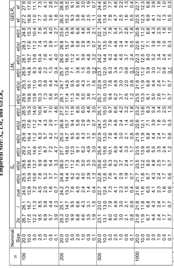
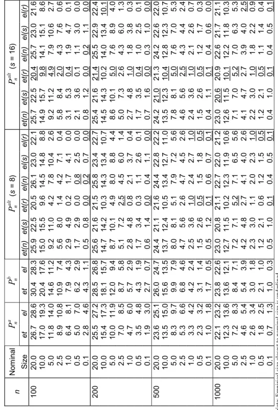
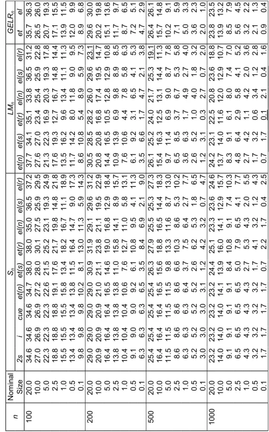
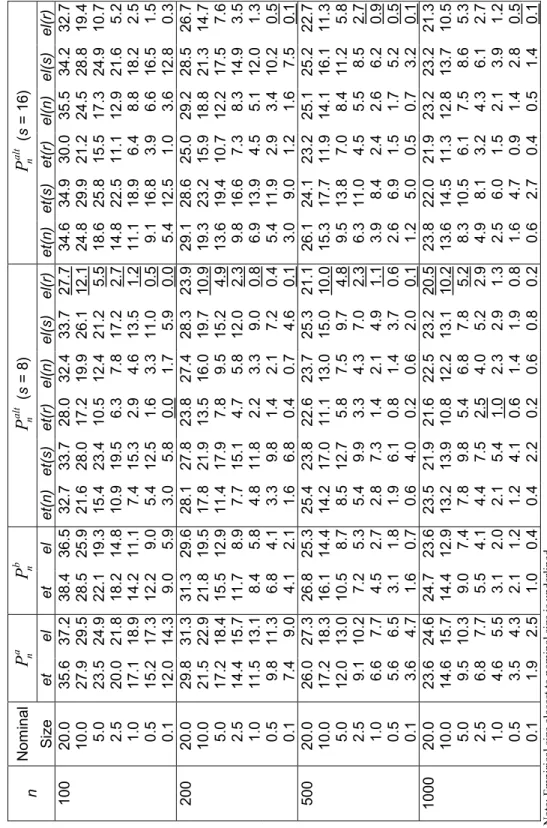
Tables 1 and 2, for the asset-pricing model, and 3 and 4, for the chi-square moments case, report the estimated size of each test at seven different levels of significance 0.200, 0.100, 0.050, 0.025, 0.010, 0.005 and 0.001. For each significance level, sample size and model considered, the actual size closest to the nominal size is underlined.
Tables 1, 2, 3 and 4 about here
The results displayed in Tables 1 and 3 conform with those presented by Imbens, Spady and Johnson (1998) for the tests analyzed in their paper.6 They show that all these tests are significantly oversized in almost all cases, even when n = 1000, particularly for the chi-square moments model. The statistic LMnet(r) registers the best behaviour in
most experiments, the only exceptions being for the largest nominal sizes, where Scue n ,
in the first model, and LMnel(r), in both models, achieve superior performances. The
size behaviour of the Sn statistic evaluated at the two-step GMM estimator, which is
most commonly used to assess overidentifying moment condition models, is generally disastrous in these experiments. In particular, it is the worst of all versions [Sn2s, Sni,
Sncue, S et(n)
n and Snel(n)] using the sample mean estimator for Ω in the asset-pricing model.
The GELRn tests also produced very modest results, with the EL version performing
substantially better than that using ET, particularly for the chi-square moments model and for the smallest nominal sizes.
As noted by Imbens, Spady and Johnson (1998), estimation of the variance matrix Ω exerts a decisive influence on the performance of the tests. However, the extraordinary benefits from the use of robust estimation reported there for the Lagrange multiplier statistic LMnet(r) do not extend to all tests, not even to LMnel(r) for the smallest nominal
sizes considered. The size behaviour of the score statistic Sn also deteriorates
consider-ably. Although a theoretical analysis of the effects of using robust estimation is beyond
6The following correspondence holds between the notation used here and that utilized by Imbens,
Spady and Johnson (1998): S2sn = Tg1AM, Sin = Tg2AM, Sncue = Tg3AM, Snet(s) = TetAM, LM
et(s)
n = Tet(s)LM,
the scope of this paper, it is clear that LMn and Sn are affected in an opposite manner
because an estimator for Ω appears as an inverse in the latter statistic.
Estimated sizes for the Pearson-type statistics are reported in Tables 2 and 4. The Pa
n and Pnb statistics perform very modestly, being substantially oversized in all cases.
Their size behaviour does not differ much from that described above for the other tests.7
In contradistinction, however, Palt
n is more promising. Whichever number of classes
s is chosen, the general effects of evaluation at different estimators are similar in all cases. Analogously to LMn, the least number of rejections of the null hypothesis occurs
when robust estimation of Ω is employed. This is unsurprising since Ω appears in the expressions for both tests in a similar manner. Overall, robust et(r) and el(r) versions of Palt
n record most of the best size properties.
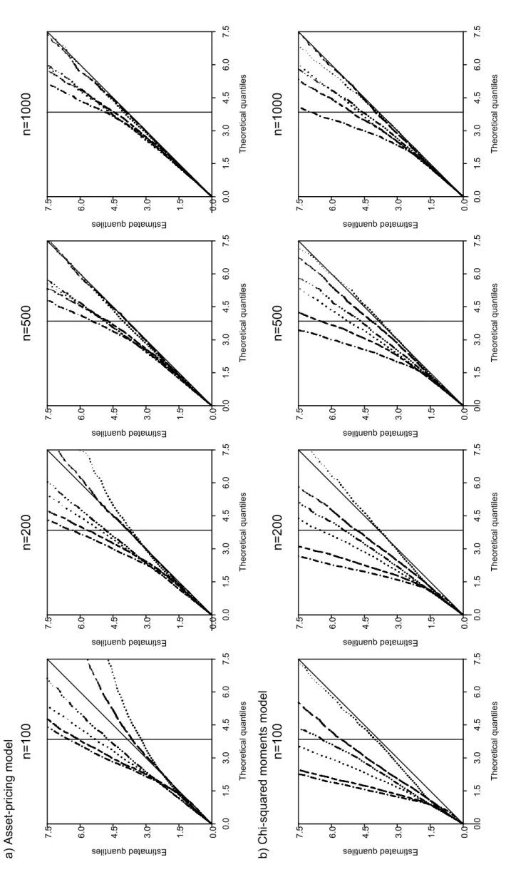
Figure 1 about here
Figure 1 displays QQ-plots comparing the six versions of Palt
n for s = 8. Vertical
coordinates are Monte Carlo estimates of quantiles of the finite sample distribution of those statistics and horizontal coordinates are quantiles of a chi-square variable with one degree of freedom. The vertical solid line marks the asymptotic critical value for a nominal size of 0.05. Clearly, the best performances are obtained by Pnalt,et(r) and
Pnalt,el(r). Note that for n≥ 500 (first model) or n = 1000 (second model) the estimated
and asymptotic quantiles of these statistics are very close while other versions of Palt n
are still significantly oversized. It is also worthy of notice how, for small sample sizes, all three EL versions of Palt
n tend to reject significantly less than the corresponding ET
variants.
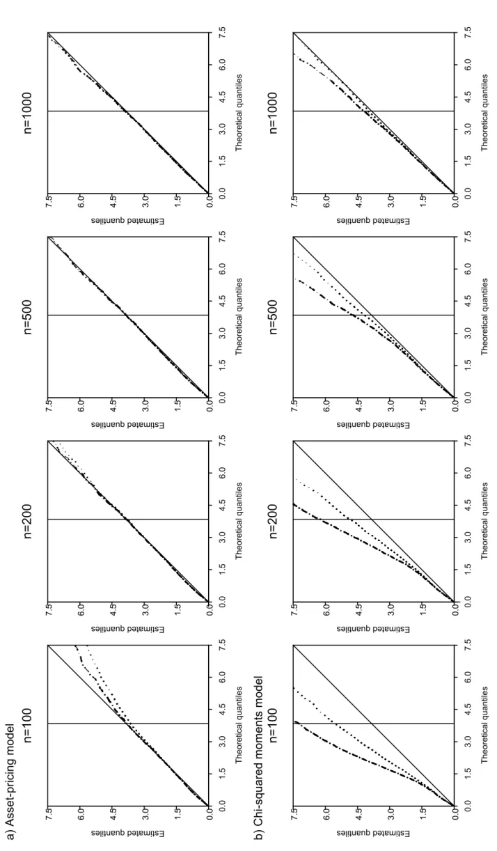
Figure 2 about here The size performance of Palt
n did not appear to be affected significantly by s for
different sample sizes. This was particularly evident for the asset-pricing model case.
7The estimated sizes for the EL version of Pb
ntest are numerically equal to those calculated for S
el(s) n
and LMnel(s). This is due to the particular form assumed by the EL implied probabilities (3.4): ˆπi =
n−1(1 + ˆλ0g
i( ˆβ))−1, (i = 1, ..., n). For example, as ˆλ0gi( ˆβ) = nˆπi − 1 and ˆΩ = Pni=1πˆigi( ˆβ)gi( ˆβ)0,
For the chi-squared moment model the differences between s = 8 and s = 16 cases were more important but were attenuated by increasing sample size. Figure 2 illustrates this situation for Pnalt,et(r) displaying QQ-plots for both values of s.
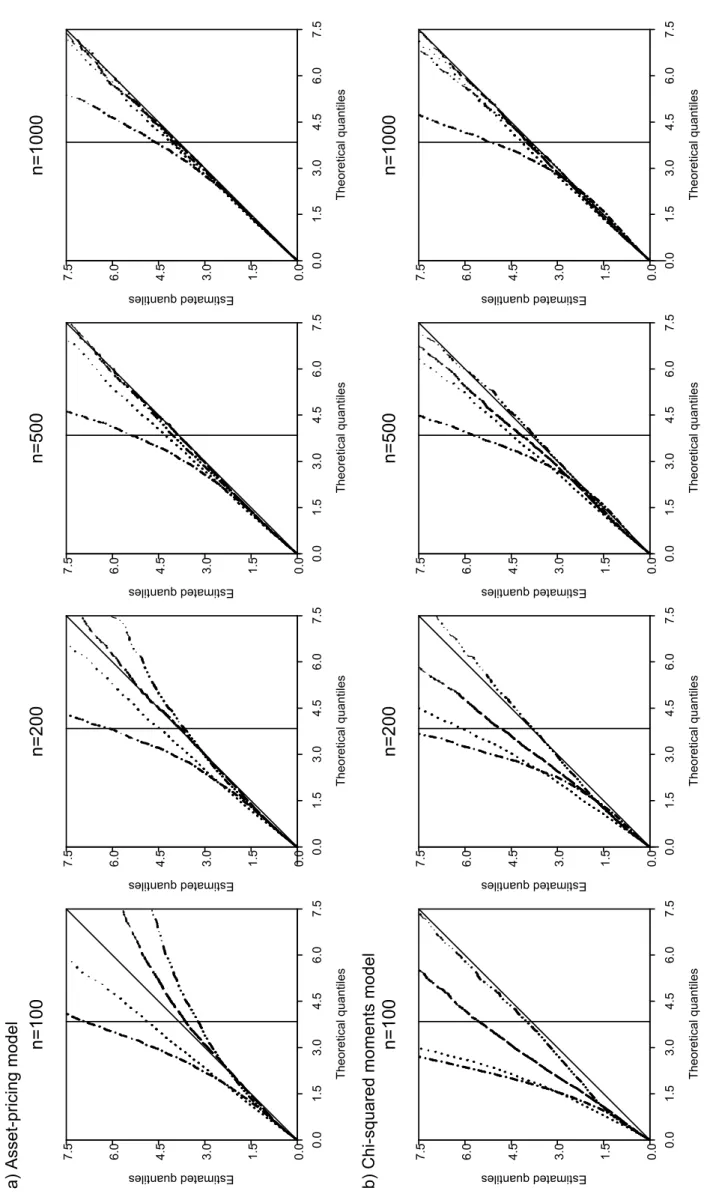
Figure 3 about here
Figure 3 compares the robust forms of LMn and Pnalt for s = 8 evaluated at ET and
EL estimators. Of the statistics considered by Imbens, Spady and Johnson (1998) and here LMnet(r) registered the best behaviour. The statistic Pnalt clearly performs better
for both models with estimated and asymptotic quantiles being closer in most cases. Furthermore, while Palt
n is relatively indifferent to the use of ET or EL estimation, at
least for the larger sample sizes, EL estimation does not work well for LMn, even for
n = 1000.
6
Conclusions
This paper develops new Pearson-type statistics appropriate for testing over-identifying moment conditions and parametric restrictions. The Pearson-type statistic contructed using a partition of the sample space performed very well in Monte Carlo simulation experiments comparing tests for over-identifying moment conditions. The size behaviour for this statistic based on robust estimation of the moment indicator variance matrix appears to be superior to that of alternative competitor tests. Moreover, this statistic seems to be insensitive to the number of classes comprising the partition of the sample space.
Appendix: Proofs
Throughout the Appendix, with probability approaching one will be abbreviated as w.p.a.1, UWL will denote a uniform weak law of large numbers such as Lemma 2.4 of Newey and McFadden (1994), CS Cauchy-Schwartz and CLT will refer to the Lindeberg-L´evy central limit theorem.
Lemma A.1 If Assumptions 2.1, 2.2 and 2.3 are satisfied, then nˆπi = 1 + op(1) and n1/2 µ ˆ πi− 1 n ¶ = 1 nˆg 0 in 1/2λ(1 + oˆ p(1)) + Op(n−3/2), uniformly (i = 1, ..., n).
Proof: Let bi = supβ∈Bkgi(β)k. From the Proof of Lemma A1 and Theorem 3.1 in
NS, as max1≤i≤nbi = Op(n 1 α) and ˆλ = Op(n−1/2), sup β∈B,1≤i≤n ¯ ¯ ¯ˆλ0g i(β) ¯ ¯ ¯ = Op(n−( 1 2− 1 α)). A first order order Taylor expansion for ρ1(ˆλ0gˆi) yields
ρ1(ˆλ0gˆi) =−1 + ρ2( ˙λ0gˆi)ˆλ0ˆgi,
where ˙λ is on the line joining ˆλ and 0. Now, max1≤i≤n ¯ ¯ ¯ρ2( ˙λ0ˆgi) + 1 ¯ ¯ ¯→ 0 as supp β∈B,1≤i≤n ¯ ¯ ¯ ˙λ0g i(β) ¯ ¯ ¯→p 0 and so ρ2( ˙λ0gˆi)ˆλ0gˆi =−ˆλ0gˆi(1 + op(1)) uniformly (i = 1, ..., n). Therefore,
ρ1(ˆλ0ˆgi) =−1 − ˆλ0ˆgi(1 + op(1)), (A.1) uniformly (i = 1, ..., n). Similarly, 1 Pn j=1ρ1(ˆλ0ˆgj) = −1 n− 1 n à n X j=1 ρ2( ˙λ0gˆj)ˆg0j/n ! ˆ λ = −1 n(1 + Op(n −1)),
asPnj=1ˆgj/n = Op(n−1/2) by Theorem 3.1 of NS. Combining eqs. (A.1) and (A.2)
ˆ πi = 1 n(1 + ˆλ 0gˆ i(1 + op(1)))(1 + Op(n−1))
and, therefore, from Lemma A1 of NS,
nˆπi− 1 = ˆλ0ˆgi(1 + op(1)) + Op(n−1) = op(1) uniformly (i = 1, ..., n). Similarly n1/2 µ ˆ πi− 1 n ¶ = 1 nˆg 0 in 1/2λ(1 + oˆ p(1)) + Op(n−3/2),
uniformly (i = 1, ..., n).
Proof of Lemma 3.1: By Lemma A.1 and noting from Theorem 3.2 of NS that n1/2ˆλ = −P n1/2ˆg(β 0) + op(1), n1/2[ˆµn(z)− µn(z)] = n1/2 n X i=1 µ ˆ πi− 1 n ¶ 1(zi ≤ z) = n X i=1 [n−1ˆgi0n1/2λ(1 + oˆ p(1)) + Op(n−3/2)]1(zi ≤ z) = à n X i=1 1(zi ≤ z)ˆgi0/n ! n1/2λ(1 + oˆ p(1)) + Op(n−1/2) = [b(z) + Op(n−1/2)]0n1/2ˆλ + op(1) ⇒ ˆΛ(z)
where ˆΛ is Gaussian stochastic process on Rk with mean zero and covariance function E[ ˆΛ(z1)ˆΛ(z2)] = b(z1)0P b(z2).
Proof of Theorem 3.1: Our method of proof is to demonstrate that the statistics Pa
n (3.7) and Pnb (3.8) are asymptotically equivalent to the Lagrange multiplier test LMn
(3.2) for the over-identifying moment conditions (2.1). Using Lemma A.1 (nˆπi− 1)2 = (ˆλ0gˆi(1 + op(1)) + Op(n−1))2,
uniformly (i = 1, ..., n). Summing over i = 1, ..., n,
n X i=1 (nˆπi− 1)2 = nˆλ0( n X i=1 ˆ giˆgi0/n)ˆλ(1 + op(1)) + n1/2ˆλ0( n X i=1 ˆ gi/n1/2)(1 + op(1))Op(n−1) +Op(n−1) = nˆλ0( n X i=1 ˆ giˆgi0/n)ˆλ + op(1) = LMn+ op(1).
From Lemma A.1,
n X i=1 (nˆπi− 1)2 = n X i=1 (nˆπi− 1)2 nˆπi + op(1).
Proof of Theorem 3.2: From a UWL, the matrix estimators ˆBs, ˆG and ˆΩ are
consistent estimators for their population counterparts Bs, G and Ω. From the Proof of
Lemma 3.1, n1/2(ˆµs n− µsn) = Bs0n1/2λ + oˆ p(1) =−Bs0P n1/2ˆg(β0) + op(1) and thus n1/2(ˆµsn− µ s n) d → N(0, Bs0P Bs).
If rk(Bs) = m then Bs0(BsBs0)−1Ω(BsBs0)−1Bs is a g-inverse for Bs0P Bs as P ΩP = P .
Therefore, Pnalt = n(ˆµ s n− µ s n)0Bs0(BsBs0)−1Ω(BsBs0)−1Bs(ˆµsn− µ s n) + op(1) = nˆg(β0)0P ΩP ˆg(β0) + op(1) = LMn+ op(1), as P ΩP = P .
Proof of Theorem 3.3: From Assumption 3.1, it follows by standard consistency results for concave objective functions (e.g. Newey and McFadden, 1994, Theorem 2.7) that ˆλ(β) = arg maxλ∈ˆΛn(β)P (β, λ) exists w.p.a.1 and ˆˆ λ(β) → λ(β). By a UWLp supβ∈B ° ° ° ˆP (β, ˆλ(β))− ρ(β, λ(β)) ° °
°→ 0. Therefore, the GEL estimator ˆp β → βp ∗ using e.g. Theorem 2.1 of Newey and McFadden (1994). As V is bounded, Pni=1ρ1(λ0gi(β))/n
p → E[ρ1(λ0g(z, β))|λ0g(z, β)∈ V] and Pn i=1ρ1(λ0gi(β))2/n p → E[ρ1(λ0g(z, β))2|λ0g(z, β) ∈ V]
uniformly β and λ. Therefore, by a UWL,Pni=1ρ(ˆλ0gˆi)/n p
→ E[ρ1(λ0∗g(z, β∗))|λ0∗g(z, β∗)∈
V] andPni=1ρ(ˆλ0gˆi) 2/n p
→ E[ρ1(λ0∗g(z, β∗))2|λ0∗g(z, β∗)∈ V]. Consider the statistic Pna.
n−1Pna = n X i=1 (nˆπi− 1) 2 /n = Pn i=1ρ1(ˆλ0gˆi)2/n (Pnj=1ρ1(ˆλ0gˆj)/n)2 − 1 p → var[ρ1(λ 0 ∗g(z, β∗))|λ0∗g(z, β∗)∈ V] E[ρ1(λ0∗g(z, β∗))|λ0∗g(z, β∗)∈ V]2 > 0. Therefore, the conclusion follows as Pna
p → ∞. Similarly, for Pnb, n−1Pnb = n−1 n X i=1 (nˆπi− 1)2 nˆπi = n X i=1 ρ1(ˆλ0gˆi)/n n X i=1 1 nρ1(ˆλ0gˆj) − 1 p → E[ρ1(λ0∗g(z, β∗))2|λ0∗g(z, β∗)∈ V]E[ρ1(λ0∗g(z, β∗))−1|λ0∗g(z, β∗)∈ V] − 1 > 0
by CS so Pnb p
→ ∞.
Proof of Theorem 3.4: Follows immediately as ˆµs n− µsn
p
→ δ∗.
Proof of Proposition 4.1: The first order conditions determining the GEL and auxiliary parameter estimators ˜β and ˜λ and Lagrange multiplier estimator ˜η are
n X i=1 ρ1(˜λ0g˜i+ ˜η0r( ˜β)) gGi( ˜i( ˜β)β)0˜λ + R( ˜β)0η˜ r( ˜β) = 00 0 . (A.2)
It is immediate from eq. (A.2) that the constrained GEL estimator ˜β satisfies the para-metric constraints; viz. r( ˜β) = 0. Hence, a similar proof to that for Theorem 3.1 of NS establishes that, if Assumption 4.1 holds, ˜β → βp 0 and ˜λ
p
→ 0. Therefore, from (A.2), as max1≤i≤n
¯ ¯
¯ρ1(˜λ0gi( ˜β)) + 1
¯ ¯
¯→ 0 as in Lemma A1 of NS, using a UWL ˜p η → 0 byp Assumption 4.2 (c)(d). Arguments like those in the proof of Theorem 3.2 of NS give
n1/2g(βˆ 0) + Ωn1/2λ + Gn˜ 1/2( ˜β− β0) = op(1),
G0n1/2λ + R˜ 0n1/2η = o˜ p(1), (A.3)
Rn1/2( ˜β− β0) = op(1). (A.4)
From eq. (A.3),
n1/2η =˜ −(RΣR0)−1RΣG0n1/2λ + o˜ p(1) (A.5)
and, thus, substituting back,
KG0n1/2λ = o˜ p(1). (A.6)
Therefore, premultiplying eq. (A.3) by KG0Ω−1 and using (A.6),
KG0Ω−1n1/2g(βˆ 0) + KΣ−1n1/2( ˜β− β0) = op(1).
Hence, from eq. (A.4),
n1/2( ˜β− β0) =−KG0Ω−1n1/2ˆg(β0) + op(1). (A.7)
Substituting (A.7) back into eq. (A.3),
and, thus, from eq. (A.5),
n1/2η = (RΣR˜ 0)−1RΣG0Ω−1n1/2g(βˆ 0) + op(1), (A.9)
as RK = 0. The result follows immediately from eqs. (A.7)-(A.9) as n1/2g(βˆ 0)
d
→ N(0, Ω) by a CLT.
Lemma A.2 If Assumptions 4.1 and 4.2 are satisfied, then n˜πi = 1 + op(1),
n1/2 µ ˜ πi− 1 n ¶ = 1 n˜g 0 in 1/2λ(1 + o˜ p(1)) + Op(n−3/2), and n1/2(˜πi− ˆπi) = 1 nˆg 0 in 1/2 (ˆλ− ˜λ)(1 + op(1)) + Op(n−3/2), uniformly (i = 1, ..., n).
Proof: The first and second conclusions follow by a similar argument to that of Lemma A.1. Therefore,
n1/2(˜πi − ˆπi) = ( 1 n˜g 0 in 1/2λ˜ − 1 nˆg 0 in 1/2λ)(1 + oˆ p(1)) + Op(n−3/2) = 1 nˆg 0 in 1/2(ˆλ − ˜λ)(1 + op(1)) + Op(n−3/2) uniformly (i = 1, ..., n) as Gi(β) = Op(1), ˜β− ˆβ = Op(n−1/2) and ˜λ = Op(n−1/2).
Proof of Lemma 4.1: From Lemma A.2 and similarly to the Proof of Lemma 3.1, n1/2[˜µn(z)− µn(z)] = n1/2 n X i=1 µ ˜ πi− 1 n ¶ 1(zi ≤ z) = n X i=1 [n−1˜gi0n 1/2˜ λ(1 + op(1)) + Op(n−3/2)]1(zi ≤ z) = à n X i=1 1(zi ≤ z)˜gi0/n ! n1/2λ(1 + o˜ p(1)) + Op(n−1/2) = [b(z) + Op(n−1/2)]0n1/2˜λ + op(1) ⇒ ˜Λ(z)
where ˜Λ is Gaussian stochastic process on Rk with mean zero and covariance function E[ ˜Λ(z1)˜Λ(z2)] = b(z1)0(Ω−1− Ω−1GKG0Ω−1)b(z2) using eq. (A.8). From eq. (A.10) and
Lemma A.2 n1/2[˜µn(z)− ˆµn(z)] = n1/2 n X i=1 (˜πi− ˆπi) 1(zi ≤ z) = n X i=1 [(1 ng˜ 0 in 1/2λ˜ − n1gˆ0in1/2λ)(1 + oˆ p(1)) + Op(n−3/2)]1(zi ≤ z) = à n X i=1 1(zi ≤ z)ˆg0i/n + Op(n−1/2) ! n1/2(˜λ− ˆλ)(1 + op(1)) + Op(n−1/2) = [b(z) + Op(n−1/2)]0n1/2(˜λ− ˆλ) + op(1) ⇒ ∆(z)
where ∆ is Gaussian stochastic process on Rk with mean zero and covariance function E[∆(z1)∆(z2)] = b(z1)0Ω−1GΣR0(RΣR0)−1RΣGΩ−1b(z2) as
n1/2(˜λ− ˆλ) = −Ω−1GΣR0(RΣR0)−1RΣGΩ−1n1/2g(βˆ 0) + op(1)
using eq. (A.8) and n1/2λ =ˆ
−P n1/2g(βˆ
0) + op(1) from the Proof of Theorem 3.2 in NS.
Proof of Theorem 4.1: From Lemma A.2, it follows immediately that (n˜πi− nˆπi)2 = ((ˆλ− ˜λ)0gˆi(1 + op(1)) + Op(n−1))2,
uniformly (i = 1, ..., n). Summing over i = 1, ..., n,
n X i=1 (nˆπi− nˆπi)2 = n(ˆλ− ˜λ)0( n X i=1 ˆ gigˆ0i/n)(ˆλ− ˜λ)(1 + op(1)) +n1/2(ˆλ− ˜λ)0( n X i=1 ˆ gi/n1/2)(1 + op(1))Op(n−1) + Op(n−1) = n(ˆλ− ˜λ)0( n X i=1 ˆ gigˆ0i/n)(ˆλ− ˜λ) + op(1) = n(ˆλ− ˜λ)0Ω(ˆλ− ˜λ) + op(1) = nˆg(β0)0Ω−1GΣR(RΣR0)−1RΣGΩ−1ˆg(β0) + op(1) = nr( ˆβ)0( ˆR ˆΣ ˆR0)−1r( ˆβ) + op(1),
the first term of which is the Wald test statistic for r(β0) = 0 which has a limiting
chi-square distribution with r degrees of freedom. See Newey and West (1987) and Smith (2001, section 5). From Lemmas A.1 and A.2
n X i=1 (nˆπi− nˆπi)2 = n X i=1 (nˆπi− nˆπi)2 nˆπi + op(1) = n X i=1 (nˆπi− nˆπi)2 n˜πi + op(1).
Proof of Theorem 4.2: From Lemma 4.1, as n1/2(˜µs
n− ˆµsn) =−Bs0n1/2(˜λ−ˆλ)+op(1),
Pna,alt,r = n(˜λ− ˆλ)0GΣG0(˜λ− ˆλ) + op(1)
= nˆg(β0)0Ω−1GΣR(RΣR0)−1RΣGΩ−1g(βˆ 0) + op(1)
= nr( ˆβ)0( ˆR ˆΣ ˆR0)−1r( ˆβ) + op(1),
which from the Proof of Theorem 4.1 is asymptotically equivalent to Pa,r
n , Pnb,r and
Pc,r
n . Similarly, from Lemma 4.1, n1/2(˜µsn − ˆµns) = Bs0n1/2λ + oˆ p(1). Therefore, from
the Proof of Proposition 4.1, as n1/2λ =˜
−(Ω−1 − Ω−1GKG0Ω−1)n1/2ˆg(β
0) + op(1) and
G0(Ω−1− Ω−1GKG0Ω−1) = R0(RΣR0)−1RΣG0Ω−1,
Pnb,alt,r = nˆλ0GΣG0λ + oˆ p(1)
= nˆg(β0)0Ω−1GΣR(RΣR0)−1RΣGΩ−1g(βˆ 0) + op(1).
Proof of Theorem 4.3: The proof is very similar in outline to that of The-orem 3.3. Firstly, ˜λ(β) = arg maxλ∈˜Λn(β)P (β, λ), βˆ ∈ Br, exists w.p.a.1 and thus ˜
λ(β) → λ(β), β ∈ Bp r. Secondly, the restricted GEL estimator ˜β → βp ∗, β∗ ∈ Br. As in the Proof of Theorem 3.3, Pni=1ρ1(λ0gi(β))/n
p
→ E[ρ1(λ0g(z, β))|λ0g(z, β)∈ V] and
Pn
i=1ρ1(λ0gi(β)) 2/n p
→ E[ρ1(λ0g(z, β))2|λ0g(z, β) ∈ V] uniformly β ∈ Br and λ.
There-fore, by a UWL,Pni=1ρ(˜λ0g
i( ˜β))/n p
→ E[ρ1(λ0∗g(z, β∗))|λ0∗g(z, β∗)∈ V] andPni=1ρ(˜λ0gi( ˜β)) 2/n p
→ E[ρ1(λ0∗g(z, β∗))2|λ0∗g(z, β∗)∈ V].
Consider the statistic Pnc,r. n−1Pnc,r = n X i=1 (n˜πi− nˆπi) 2 /n = Pn i=1ρ1(˜λ0gi( ˜β))2/n (Pnj=1ρ1(˜λ0gj( ˜β))/n)2 − 2 Pn i=1ρ1(˜λ0gi( ˜β))ρ1(ˆλ0gi( ˆβ))/n (Pnj=1ρ1(˜λ0gj( ˜β))/n)(Pnj=1ρ1(ˆλ0gj( ˆβ))/n) + Pn i=1ρ1(ˆλ0gi( ˆβ))2/n (Pnj=1ρ1(ˆλ0gj( ˆβ))/n)2 = Ã Pn i=1ρ1(˜λ0gi( ˜β))2/n (Pnj=1ρ1(˜λ0gj( ˜β))/n)2 − 1 ! + op(1) p → var[ρ1(λ 0 ∗g(z, β∗))|λ0∗g(z, β∗)∈ V] E[ρ1(λ0∗g(z, β∗))|λ0∗g(z, β∗)∈ V]2 > 0.
The third equality follows as ρ1(ˆλ0g(zi, ˆβ)) = −1 + op(1), uniformly (i = 1, ..., n), from
Lemma A1 in NS, Pnj=1ρ1(ˆλ0g(zj, ˆβ))2/n p → 1 and Pnj=1ρ1(ˆλ0g(zj, ˆβ))/n p → −1. The conclusion Pc,r n p
→ ∞ is then immediate. Similarly, for Pa,r n , n−1Pna,r = n X i=1 (n˜πi− nˆπi) 2 ˆ πi = ( Pn i=1ρ1(˜λ0g˜i) 2/nρ 1(ˆλ0gˆi))(Pj=1n ρ1(ˆλ0ˆgj)/n) (Pnj=1ρ1(˜λ0˜gj)/n)2 − 1 = Ã (Pni=1ρ1(˜λ0g˜i)2/n) (Pnj=1ρ1(˜λ0g˜j)/n)2 − 1 ! + op(1) = n−1Pnc,r+ op(1). For Pb,r n , n−1Pnb,r = n X i=1 (n˜πi− nˆπi)2 ˜ πi = ( Pn i=1ρ1(ˆλ0ˆgi) 2/nρ 1(˜λ0˜gi))(Pj=1n ρ1(˜λ0g˜j)/n) (Pnj=1ρ1(ˆλ0gˆj)/n)2 − 1 p → E[ρ1(λ0∗g(z, β∗))|λ0∗g(z, β∗) ∈ V] ×E[ρ1(λ0∗g(z, β∗))−1|λ0∗g(z, β∗) ∈ V] − 1 > 0 by CS so Pnb,r p → ∞.
Proof of Theorem 4.4: Follows immediately as ˜µsn− ˆµsn p → δ∗ and ˜µsn− µsn p → δ∗.
References
Andrews, D. W. K. (1988a): “Chi-Square Diagnostic Tests for Econometric Models: Introduction and Applications”, Journal of Econometrics, 37, 135-156.
Andrews, D. W. K. (1988b): “Chi-Square Diagnostic Tests for Econometric Models: Theory”, Econometrica, 56, 1419-1453.
Back, K. and D. P. Brown (1993): “Implied probabilities in GMM estimators”, Econo-metrica, 61(4), 971-975.
Brown, B.W. and W.K. Newey (1992): “Bootstrapping for GMM”, mimeo, M.I.T. Brown, B.W. and W.K. Newey (1998): “Efficient Semiparametric Estimation of
Expec-tations,” Econometrica 66, 453-464.
Brown, B.W. and W.K. Newey (2003): “Generalised Method of Moments, Efficient Bootstrapping, and Improved Inference,” Journal of Business and Economic Statis-tics, 20, 507-517.
Cressie, N., and T. Read (1984): “Multinomial Goodness-of-Fit Tests”, Journal of the Royal Statistical Society Series B, 46, 440-464.
Durbin, J. (1973): Distribution Theory for Tests Based on the Sample Distribution Function. CBMS-NSF Regional Conference Series in Applied Mathematics No.9. SIAM: Philadelphia.
Hansen, L. P. (1982): “Large sample properties of generalised method of moments estimators”, Econometrica, 50(4), 1029-1054.
Hansen, L. P., J. Heaton and A. Yaron (1996): “Finite-sample properties of some al-ternative GMM estimators”, Journal of Business & Economic Statistics, 14(3), 262-280.
Imbens, G. W. (1997): “One-step estimators for over-identified generalised method of moments models”, Review of Economic Studies, 64, 359-383.
Imbens, G. W., R. H. Spady and P. Johnson (1998): “Information theoretic approaches to inference in moment condition models”, Econometrica 66, 333-357.
Kitamura, Y. and M. Stutzer (1997): “An information-theoretic alternative to gener-alised method of moments estimation”, Econometrica, 65(4), 861-874.
Newey, W.K. and D. McFadden (1994): “Large Sample Estimation and Hypothesis Testing,” in Engle, R. and D. McFadden, eds., Handbook of Econometrics, Vol. 4, New York: North Holland.
Newey, W. K., J. J. S. Ramalho, and R. J. Smith, (2002): “Asymptotic Bias for GMM and GEL Estimators with Estimated Nuisance Parameters”. Forthcoming in Iden-tification and Inference in Econometric Models: Essays in Honor of Thomas J. Rothenberg, eds. D.W.K. Andrews and J.H. Stock. Cambridge University Press: Cambridge..
Newey, W. K. and R. J. Smith (2001): “Higher Order Properties of GMM and Gener-alized Empirical Likelihood Estimators”, Econometrica, 72, 219-255.
Owen, A. (2001): Empirical Likelihood. New York: Chapman and Hall.
Qin, J. and J. Lawless (1994): “Empirical Likelihood and General Estimating Equa-tions”, Annals of Statistics, 22, 300-325.
Rao, C. R. and S. K. Mitra (1971): Generalized Inverse of Matrices and Its Applications. Wiley: New York.
Shorack, G.R., and J.A. Wellner (1986): Empirical Processes with Applications in Statis-tics. Wiley: New York.
Smith, R. J. (1997), “Alternative Semi-Parametric Likelihood Approaches to Gener-alised Method of Moments Estimation”, Economic Journal, 107, 503-519.
Smith, R. J. (2001): “GEL Methods for Moment Condition Models”, working paper, Department of Economics, University of Bristol.